Consistent Monocular Ackermann Visual–Inertial Odometry for Intelligent and Connected Vehicle Localization


State Key Laboratory of Automotive Simulation and Control, Jilin University, Changchun 130022, China
*
Author to whom correspondence should be addressed.
Sensors 2020, 20(20), 5757; https://doi.org/10.3390/s20205757
Submission received: 26 August 2020
/
Revised: 5 October 2020
/
Accepted: 7 October 2020
/
Published: 10 October 2020
(This article belongs to the Collection Positioning and Navigation)
Abstract
:The observability of the scale direction in visual–inertial odometry (VIO) under degenerate motions of intelligent and connected vehicles can be improved by fusing Ackermann error state measurements. However, the relative kinematic error measurement model assumes that the vehicle velocity is constant between two consecutive camera states, which degrades the positioning accuracy. To address this problem, a consistent monocular Ackermann VIO, termed MAVIO, is proposed to combine the vehicle velocity and yaw angular rate error measurements, taking into account the lever arm effect between the vehicle and inertial measurement unit (IMU) coordinates with a tightly coupled filter-based mechanism. The lever arm effect is firstly introduced to improve the reliability for information exchange between the vehicle and IMU coordinates. Then, the process model and monocular visual measurement model are presented. Subsequently, the vehicle velocity and yaw angular rate error measurements are directly used to refine the estimator after visual observation. To obtain a global position for the vehicle, the raw Global Navigation Satellite System (GNSS) error measurement model, termed MAVIO-GNSS, is introduced to further improve the performance of MAVIO. The observability, consistency and positioning accuracy were comprehensively compared using real-world datasets. The experimental results demonstrated that MAVIO not only improved the observability of the VIO scale direction under the degenerate motions of ground vehicles, but also resolved the inconsistency problem of the relative kinematic error measurement model of the vehicle to further improve the positioning accuracy. Moreover, MAVIO-GNSS further improved the vehicle positioning accuracy under a long-distance driving state. The source code is publicly available for the benefit of the robotics community.
1. Introduction
Intelligent and connected vehicles (ICVs) are a popular research topic in intelligent transportation systems [1,2]. The Global Navigation Satellite System (GNSS) is one of the most mature global positioning technologies for vehicle navigation [3]. However, the GNSS signal is vulnerable under tunnels, trees and other obstacles [4]. Providing real-time and accurate vehicle pose information in GNSS-denied environments is a necessary prerequisite for ICV navigation [5,6,7]. Visual–inertial odometry (VIO), which integrates a visual sensor and inertial measurement unit (IMU), can provide pose information with six degrees of freedom (DOF). It is widely used in the pose estimation of mobile robots owing to the advantages of favorable robustness, small size and low cost. VIO mainly consists of filter-based methods, including the Multi-Sensor Fusion Approach (MSF) [8], the Robust Visual-Inertial Odometry (ROVIO) [9], the Multi-State Constraint Kalman Filter (MSCKF) [10], Stereo-MSCKF [11], S-MSCKF [12], the Robocentric Visual-Inertial Odometry (R-VIO) [13], Schmidt-MSCKF [14], the Lightweight Hybrid Visual-Inertial Odometry (LARVIO) [15,16] and optimization-based methods including the Open Keyframe-based Visual-Inertial SLAM (OKVIS) [17], ORB-SLAM-VI [18], VINS-Mono [19], PL-VIO [20], ICE-BA [21], VI-DSO [22], VINS-Fusion [23,24], Basalt [25] and ORB-SLAM3 [26]. A detailed review of the VIO methods can be found in the literature [27,28].
However, the standard VIO is subjected to additional unobservable directions under constant acceleration and straight-line driving states or approximate combinations of the above two driving states of ground vehicles, resulting in larger pose-estimation errors [29,30,31]. To address this problem, there are some studies of integrating VIO algorithms with the information from the vehicle proprioceptive sensors, including the drive motor encoder sensor and steering wheel angle sensor. Wu et al. [30] proposed fusing wheel speed encoder measurements into VIO based on the square-root inverse sliding window filter (SR-ISWF) [32], which significantly improved positioning accuracy under special motions of ground differential steering robots. Li et al. [33] proposed a factor-graph-based, gyro-aided localization system by exploiting the wheel odometry and gyro measurements, which achieved better accuracy than ORB-SLAM [34,35]. KO-Fusion [36] was proposed to fuse the Mecanum wheel motion constraint into RGB-D SLAM for ground robots, which improved the robustness of SLAM. Zheng and Liu [37] proposed an SE(2)-constrained pose parameterization optimization-based VIO for ground vehicles, which obtained better accuracy under sharp-turn motion. Dang et al. [38] proposed a tightly-coupled VIO to fuse wheel encoder measurements by considering wheel slippage, which achieved great improvements in positioning accuracy. Quan et al. [39] proposed a tightly coupled monocular simultaneous localization and mapping (SLAM) system, VOSLAM, by integrating visual, odometer and gyroscope measurements, which ensured the system’s accuracy. The VOSLAM improved the robustness of initialization and faulty information by a map initialization method and reliable odometer measurements. Liu et al. [40] proposed a tightly coupled optimization-based VIO to combine a wheel encoder, IMU and visual sensor, which improved the robustness of initialization and positioning accuracy. To improve the positioning accuracy before the first turning in [40], Liu et al. [41] proposed a bidirectional trajectory computation method, which achieved a more accurate real-time trajectory. Zhang et al. [42] proposed a wheel odometry with motion manifold representation for ground robot localization, which achieved accurate 6D pose estimation. Ye et al. [43] proposed a robust pose estimation method with multi-camera, odometer and gyroscope measurements in a tightly coupled optimization framework, which had obvious advantages in loop-closure detection. Gang et al. [44] proposed a tightly coupled SLAM method using wheel speed, IMU and monocular vision, which solved the problem of an unobservable scale and improved the positioning robustness. Zuo et al. [45] proposed a kinematics-constrained VIO and provided detailed observability analysis for a skid-steering mobile robot, and the experimental results showed that the kinematic parameters were observable under general motion and online kinematic parameter estimation can significantly improve positioning accuracy. VINS-Vehicle [46] was proposed to fuse two DOF vehicle dynamics models into VIO based on the sliding window optimization method, which significantly enhanced the robustness and accuracy compared with existing VIO methods. Lee et al. [47] proposed a visual-inertial-wheel odometry system, VIWO, by integrating the measurements of IMU, camera and wheel odometry preintegration, which provided theoretical guidance for the localization of ground differential steering vehicle.
By integrating the information from the vehicle proprioceptive sensors, the above tightly coupled VIO methods can improve the observability of the VIO scale direction and further enhance the vehicle positioning accuracy. However, apart from in [46], the above methods have not taken enough advantage of the measurements from the steering wheel angle sensor, which is a low-cost built-in sensor in ICVs. Moreover, the above methods except [30,47] adopt an optimization-based backend, which requires higher computational complexity. In view of the efficient performance, the Ackermann Multi-State Constraint Kalman Filter (ACK-MSCKF) [48] was proposed for integrating Ackermann error state measurements and S-MSCKF in a tightly coupled filter-based mechanism in our previous work, which improved the positioning accuracy under degenerate motions of ground vehicles. However, it adopts a stereo configuration, which is more costly and less computationally efficient than monocular solutions. Moreover, it assumes that the vehicle velocity is constant between two consecutive camera states, which degrades the positioning accuracy. Lastly and most importantly, the observability, consistency and positioning accuracy of different parameter configurations of ACK-MSCKF with vehicle relative kinematic error measurements need to be further explored.
Therefore, in this paper, a tightly coupled filter-based consistent monocular Ackermann VIO, termed MAVIO, is proposed to combine the vehicle velocity and yaw angular rate error measurements, considering the lever arm effect between the vehicle and IMU coordinates. Similar to in the work [49], to obtain a global position for the vehicle, the raw GNSS error measurement model, termed MAVIO-GNSS, is introduced to further improve the performance of MAVIO. The famous open-source VIO, i.e., S-MSCKF [12], is adopted as the base of this work. The main contributions of this paper are highlighted as follows:
- (1)
- Additional analyses of different parameter configurations of ACK-MSCKF are performed with more real-world experiments.
- (2)
- Conducting the formulation and implementation of a consistent monocular Ackermann VIO, MAVIO, which not only improves the observability of the VIO scale direction but also resolves the inconsistency problem of ACK-MSCKF for further improving the positioning accuracy.
- (3)
- Introducing the raw GNSS error measurement model, MAVIO-GNSS, which further improves the vehicle positioning accuracy under the long-distance driving state.
- (4)
- The performance of MAVIO and MAVIO-GNSS are comprehensively compared with S-MSCKF and ACK-MSCKF on real-world datasets with twenty rounds, on average, of real-world experiments.
- (5)
- The source code [50] of MAVIO is publicly available to facilitate the reproducibility of related research.
The remainder of this paper is structured as follows: The proposed approach is introduced in detail in Section 2. Then, Section 3 describes how the real-world experiments were carried out. Besides, the experimental results are discussed in Section 4. Finally, Section 5 presents the conclusions drawn.
2. The Proposed Approach
2.1. Coordinate Systems and Notations
The Vehicle Coordinate System {B}, IMU Coordinate System {I} and Camera Coordinate System {C} had the same definitions as in [48]. The additional four coordinate systems were defined as follows:
- (1)
- Inertial Coordinate System of IMU {GI}. The origin of {GI} is the same as that of {I} at the time of VIO initialization. The axes of {GI} are obtained by calculation at the time of VIO initialization, and its z-axis is aligned with Earth’s gravity.
- (2)
- Inertial Coordinate System of Vehicle {GB}. The origin of {GB} is the same as that of {B} at the time of VIO initialization. The axes of {GB} are obtained by calculation at the time of VIO initialization, and its z-axis is aligned with Earth’s gravity.
- (3)
- GNSS Coordinate System {S}. The origin of {S} lies in the center of the GNSS equipment. The x-axis and y-axis point forward and to the right, respectively, following the right-hand rule.
- (4)
- Universal Transverse Mercator Coordinate System {US}. The {US} is a universal global coordinate system. Please refer to [51] for more details.
2.2. The Lever Arm Effect between the Vehicle and IMU Coordinates
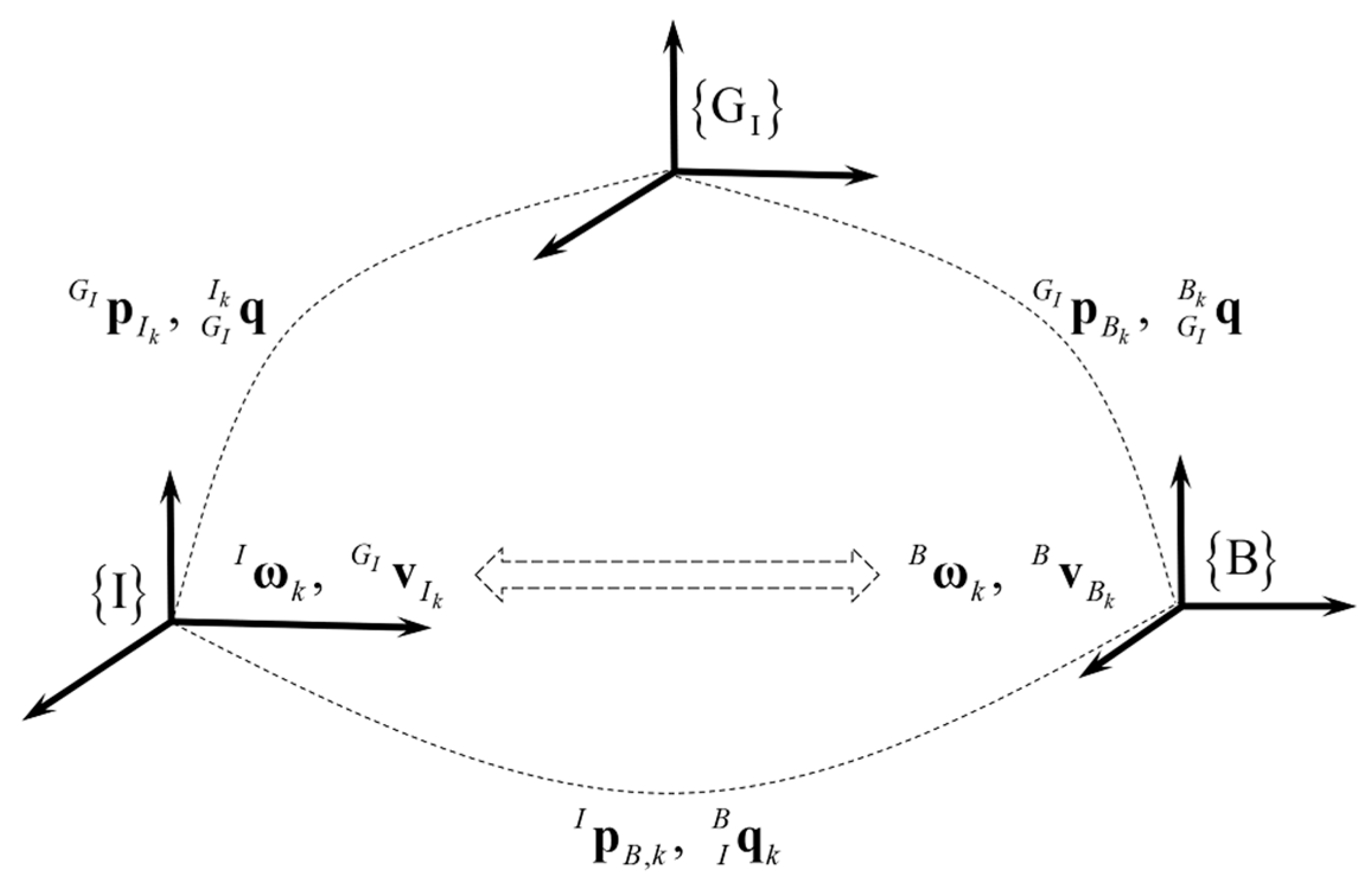
In the practical application of VIO systems for vehicles, the IMU and camera are usually installed on the front of the vehicle. Due to the existence of translation extrinsic parameters between {B} and {I}, the lever arm effect between {B} and {I} cannot be negligible. The lever arm effect between {B} and {I} is shown in Figure 1.
According to the presentation of the lever arm effect in [54], the vehicle velocity at time is derived as
where denotes the lever arm velocity at time between {B} and {I}, and are defined as
and the vehicle angular rate at time is derived as
where denotes the relative angular rate between {B} and {I}, which can be negligible with a fixed installed location for the IMU.
2.3. Process Model and Monocular Visual Measurement Model
The vehicle state vector at the sampling time for the IMU is defined as [54]
where denotes the rotation quaternion from {GB} to {B} at time . denotes the position of {B} in {GB}. denotes the velocity of {I} in {GB}. and denote the rotation and translation extrinsic parameters between {B} and {I} at time , respectively. The symbols and denote the gyroscope and accelerometer biases of the IMU at time , respectively.
Following Equation (4), the error state vector at time is defined as
The continuous-time kinematic differential equations of the true state are
where and denote the random-walk noises of the gyroscope and accelerometer biases at time , respectively. The true IMU angular rate and acceleration at time are represented as
where and denote the Gaussian white noises of the gyroscope and accelerometer measurements at time , respectively.
According to Equation (6), the linearized continuous-time kinematic differential equation of the error state at time follows
where denotes the continuous-time input noise vector. and are the continuous-time error-state transition matrix and input noise Jacobian matrix at time , respectively. and are represented as
where the analytical expressions of each block matrix in and are derived as described in Appendix A.
The camera state at the sampling time of camera is defined as
where denotes the rotation quaternion from {GB} to {C} at time and is the position of {C} in {GB}. At , and are given by
According to Equation (4) and Equation (11), the full state vector with camera states at time is given by
Following Equation (13), the full error state vector at time is defined as
2.4. Kinematic Error Measurement Model for Vehicle
2.4.1. Measurements of Vehicle Relative Kinematic Error
The refined measurement Jacobian matrix of the vehicle relative kinematic errors in Equation (18) of [48] is represented as
where denote the measurement Jacobian block matrixes of the vehicle relative rotation errors; denote the measurement Jacobian block matrixes of the vehicle relative translation errors; and their analytical expressions are derived as described in Appendix B.
Considering the fact that the measurements of vehicle kinematic error originate from the vehicle velocity, angular rate, and the characteristics of the vehicle relative kinematic errors between two consecutive camera states, the method using a kinematic error measurement model for the vehicle has different parameter configurations in practical application. Therefore, following Equation (15), the tunable parameter configurations of ACK-MSCKF are as shown in Table 1.
2.4.2. Measurements of Vehicle Velocity and Angular Rate Error
The limitation of the above relative kinematic error measurement model for the vehicle derives from the assumption that the vehicle velocity is constant for low-speed motion between two consecutive camera states. To address this problem, the vehicle velocity and yaw angular rate error measurement model, taking into account the lever arm effect between {B} and {I}, is presented as one of the primary contributions of this paper.
The measurement residual at time is defined as
where and denote the vehicle velocity measurement residual and angular rate measurement residual at time in {B}, respectively. and denote the vehicle velocity and angular rate measurements at time in {B}, respectively. and denote the vehicle velocity and angular rate estimations at time in {B}, respectively.
Considering the nonholonomic constraint of ground vehicles [54], and are represented as
where and denote the vehicle’s longitudinal speed and the yaw angular rate measurements at time in {B}, respectively. can be obtained from the vehicle controller area network-bus (CAN-bus), and is represented as
where denotes the steering radius at time ; it can be obtained according to the Ackermann steering geometry [55]:
Following Equation (19), is represented as
where denotes the steering radius at time . and denote the wheel base and the distance between the steering king pins, respectively, which can be acquired from manual measurement. denotes the outer front wheel steering angle at time , which is represented as
where denotes the steering angular transmission ratio obtained from the offline calibration. denotes the steering wheel angle at time , which can also be obtained from the vehicle CAN-bus.
Based on the lever arm effect between {B} and {I}, and are represented as
By linearizing Equation (16) at current error state , is approximated as
where denotes the measurement noise vector at time :
where denote the measurement noises of , and denote the measurement noises of . The measurement covariance matrix of is given by
where denote the standard deviations of the measurement noise. denotes the variance of at time ; it is obtained by
where denotes the variance of additional uncertain noise, and denotes the covariance matrix of the input noise:
where denotes the standard deviation of the outer front wheel steering angle.
in Equation (26) denotes the Jacobian matrix of the input noise; it is represented as
where
in Equation (23) represents the measurement Jacobian matrix of vehicle velocity and angular rate errors; it is derived as
where denote the measurement Jacobian block matrixes of the vehicle angular rate errors; denote the measurement Jacobian block matrixes of the vehicle velocity errors; and their analytical expressions are derived as described in Appendix C.
Following Equation (30), the tunable parameter configurations of MAVIO are shown in Table 2.
Following Equations (8) and (23), the updated covariance matrix and state vector of MAVIO at time are obtained by using the standard extended Kalman filter (EKF).
2.5. Raw GNSS Error Measurement Model
To obtain a global position for the vehicle, the raw GNSS error measurement model is proposed to further refine the estimator after the process of MAVIO(1).
The measurement residual at time is defined as
where and denote the measured and estimated values of {S} in {US} at time , respectively. can be converted from the raw latitude and longitude of the dual-antenna Spatial NAV982-RG inertial navigation system without the carrier-phase based differential process by using the robot_localization [56] process. is derived as
where denotes the rotation quaternion from {US} to {GB}. denotes the position of {GB} in {US}. denotes the translation extrinsic parameter between {S} and {I}.
By linearizing Equation (32) at current error state , is approximated as
where denotes the measurement noise vector of the raw GNSS data at time . represents the measurement Jacobian matrix of the raw GNSS errors; it is derived as
where denote the measurement Jacobian block matrixes of the raw GNSS errors, and their analytical expressions are derived as described in Appendix D.
Following Equations (8) and (33), the updated covariance matrix and state vector of MAVIO-GNSS at time are obtained by using the standard extended Kalman filter (EKF).
3. Experiments and Results
3.1. Experimental Vehicle Platform and Real-World Datasets
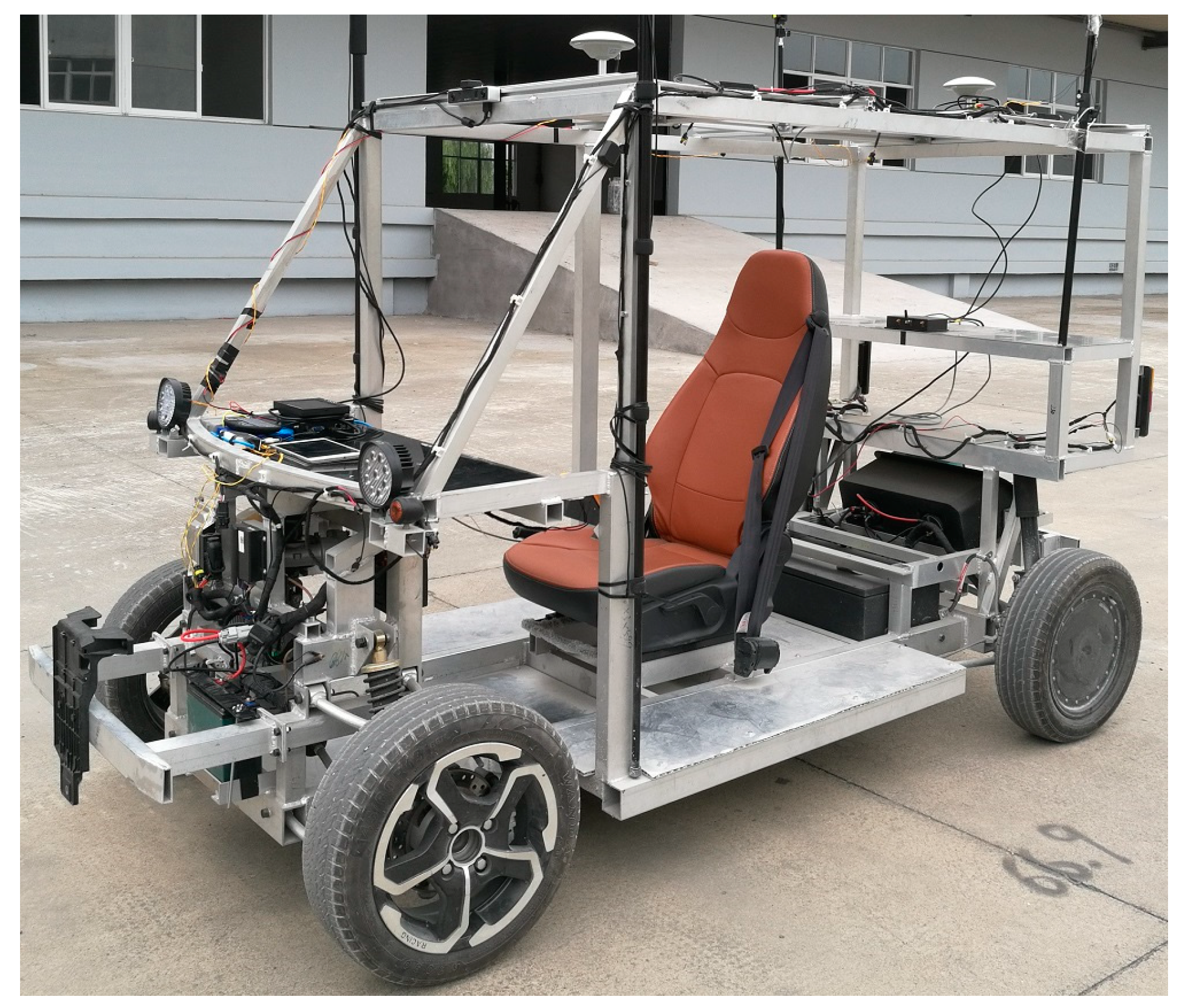
The real-world experiments were performed with a medium-size Ackermann steering vehicle, i.e., Vehicle_a27, which is shown in Figure 2. For further details of the experimental vehicle setup, please refer to [48].
Taking into account the different vehicle driving states and travel distances, six different real-world experimental datasets were acquired by using Vehicle_a27, i.e., the VD01 dataset, VD02 dataset, VD03 dataset, VD04 dataset, VD05 dataset and VD06 dataset. The VD01 dataset and VD02 dataset were, respectively, acquired under a straight-line driving state and an S-shaped-curve driving state. The VD03 dataset was acquired under a circular-curve driving state for five circles. The VD04 dataset was acquired under straight-line and turning driving states by traveling around the building in a test field for one circle. The VD05 dataset was acquired under S-shaped-curve, straight-line and turning driving states by traveling around the building in a test field for one circle. The VD04 and VD05 datasets correspond to the AM_01 and AM_02 datasets in [48], respectively. The VD06 dataset was acquired under straight-line and turning driving states by traveling around the building in a test field for three circles. The details of the real-world experimental datasets are shown in Table 3.
Figure 3 shows the ground-truth vehicle longitudinal speeds for the real-world datasets.
Figure 3 indicates that the ground-truth vehicle longitudinal acceleration was close to a constant value in short periods of time for all of the real-world datasets, which provides potential support for the data with degenerate motions of ground vehicles.
3.2. Experimental Results
Considering the differences between each round of real-world experimental results caused by the non-real-time computer operating system and other uncertain factors, the performance of MAVIO and MAVIO-GNSS were compared with S-MSCKF and ACK-MSCKF using real-world datasets by averaging all twenty rounds of experimental results. The arithmetic mean was adopted for the averaging of many rounds of vehicle position and root mean square scale ratio data. For the average of the vehicle attitude data, the weighted average quaternion [57] was used. For qualitative and quantitative positioning accuracy evaluation, the estimated trajectory, absolute trajectory error (ATE), relative translation error (RTE) and relative translation error percentage (RTEP) were calculated based on the average results by using the rpg_trajectory_evaluation [58] package. Owing to this operation, the results in this paper are more convincing. The source code for the data average processing can be publicly accessed from [59].
For consistency of comparison, we adopted the ground-truth pose errors and estimated (triple standard deviation) bounds [60] along with time in one round of experiments. For observability comparisons for scale direction, the root mean square scale ratio (RMSSR) at time was used as an evaluation index. The smaller the root mean square scale ratio , the more consistent the estimated scale of the positioning trajectory with the real scale [54]. is defined as
where denotes the number of output pose estimation results. denotes the scale ratio [30] at time
where,
where and denote the estimated positions of {B} in {GB} at time and , respectively. and denote the ground-truth positions of {B} in {GB} at time and , respectively.
and are initialized by the trajectory alignment method [61]; the open source code [62] is referenced in the implementation of the trajectory alignment. For simplicity, the origin of {B} coincides with that of {S}. The initial translation extrinsic parameter vector between {B} and {I} is obtained by manual measurement. The initial rotation extrinsic parameter vector between {B} and {I} was calibrated by the method proposed in Section 2.4 of [48]. Taking into account the effects of vehicle vibration and temperature changes, the IMU noise parameters calibrated with the kalibr_allan [63] package were expanded by 10 times in all the real-world experiments.
3.2.1. Observability and Consistency Comparison
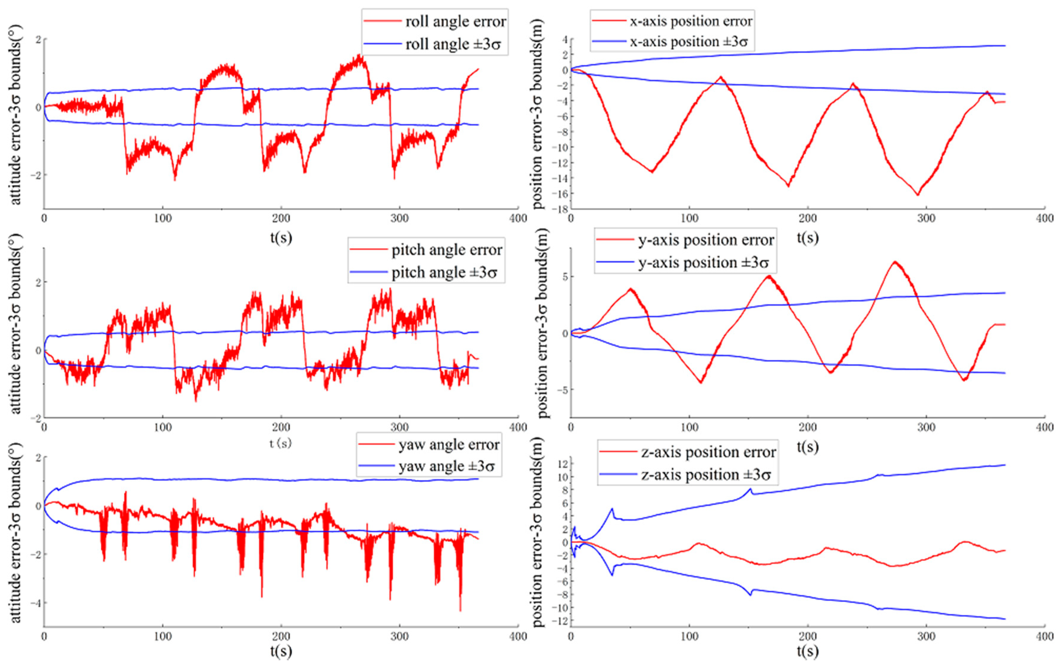
Figure 4 and Figure 5 show the ground-truth pose errors and estimated bounds of ACK-MSCKF(1) and ACK-MSCKF(2) with time, respectively.
Figure 4 and Figure 5 show that the estimated three-axis position standard deviation of ACK-MSCKF(1) and ACK-MSCKF(2) with time for the VD06 dataset is close to zero, and the estimated three-axis attitude angle standard deviation tends to be constant with time. These results indicate that the three-axis vehicle position error state and attitude angle error state are both observable. Actually, the vehicle relative kinematic error measurements do not provide information on the vehicle yaw angle and three-axis position in {GB}. Therefore, ACK-MSCKF(1) and ACK-MSCKF(2) obtain spurious information along the direction of the vehicle yaw angle and three-axis position, which leads to an inconsistency problem in that the ground-truth errors of the vehicle yaw angle and three-axis position are far greater than their estimated with time.
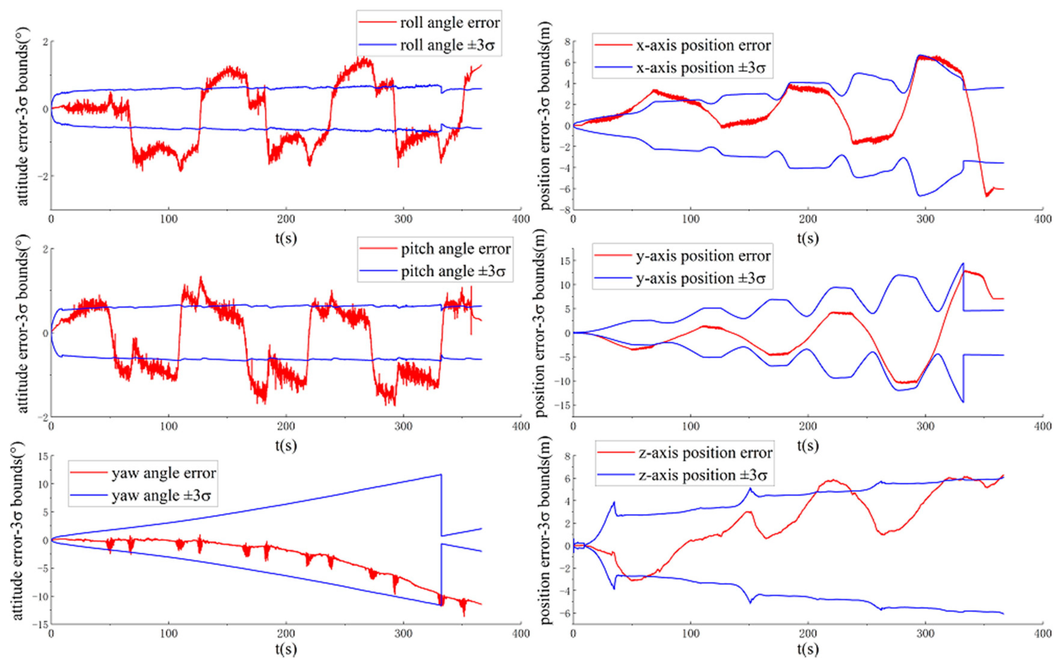
Figure 6 and Figure 7 show the ground-truth pose errors and estimated bounds of ACK-MSCKF(3) and ACK-MSCKF(4) with time, respectively.
Similarly, it is seen from Figure 6 and Figure 7 that ACK-MSCKF(3) and ACK-MSCKF(4) are subjected to the same problem as above, especially along the direction of the vehicle yaw angle. From the above analysis, there appears the problem of estimator inconsistency in all the tunable parameter configurations of ACK-MSCKF.
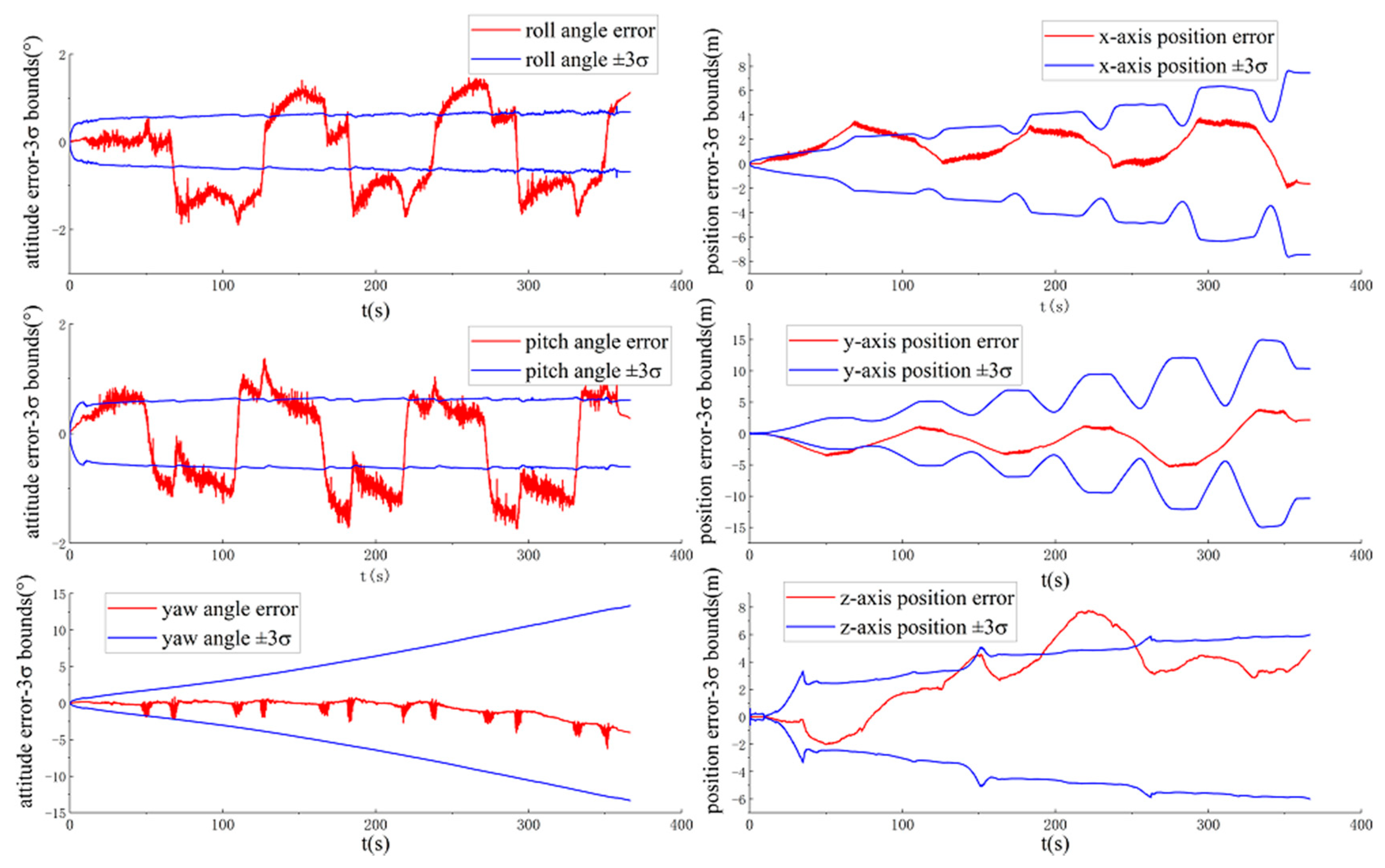
Figure 8 and Figure 9 show the ground-truth pose errors and estimated bounds of MAVIO(1) and MAVIO(2) with time, respectively.
It is concluded from Figure 8 and Figure 9 that the estimator of MAVIO(1) and MAVIO(2) is consistent according to the fact that the ground-truth errors of the vehicle yaw angle and three-axis position are enclosed in their estimated with time. Moreover, the three-axis vehicle position error state and yaw angle error state of the different parameter configurations of MAVIO are unobservable, which agrees with the result of the existing VIO observability analysis [64]. Therefore, MAVIO can overcome the inconsistency problem of ACK-MSCKF by introducing the vehicle velocity and angular rate error measurements, which could have a positive effect on improving positioning accuracy. Note that the reset phenomenon of the estimated is attributed to the robust implementation of S-MSCKF [12].
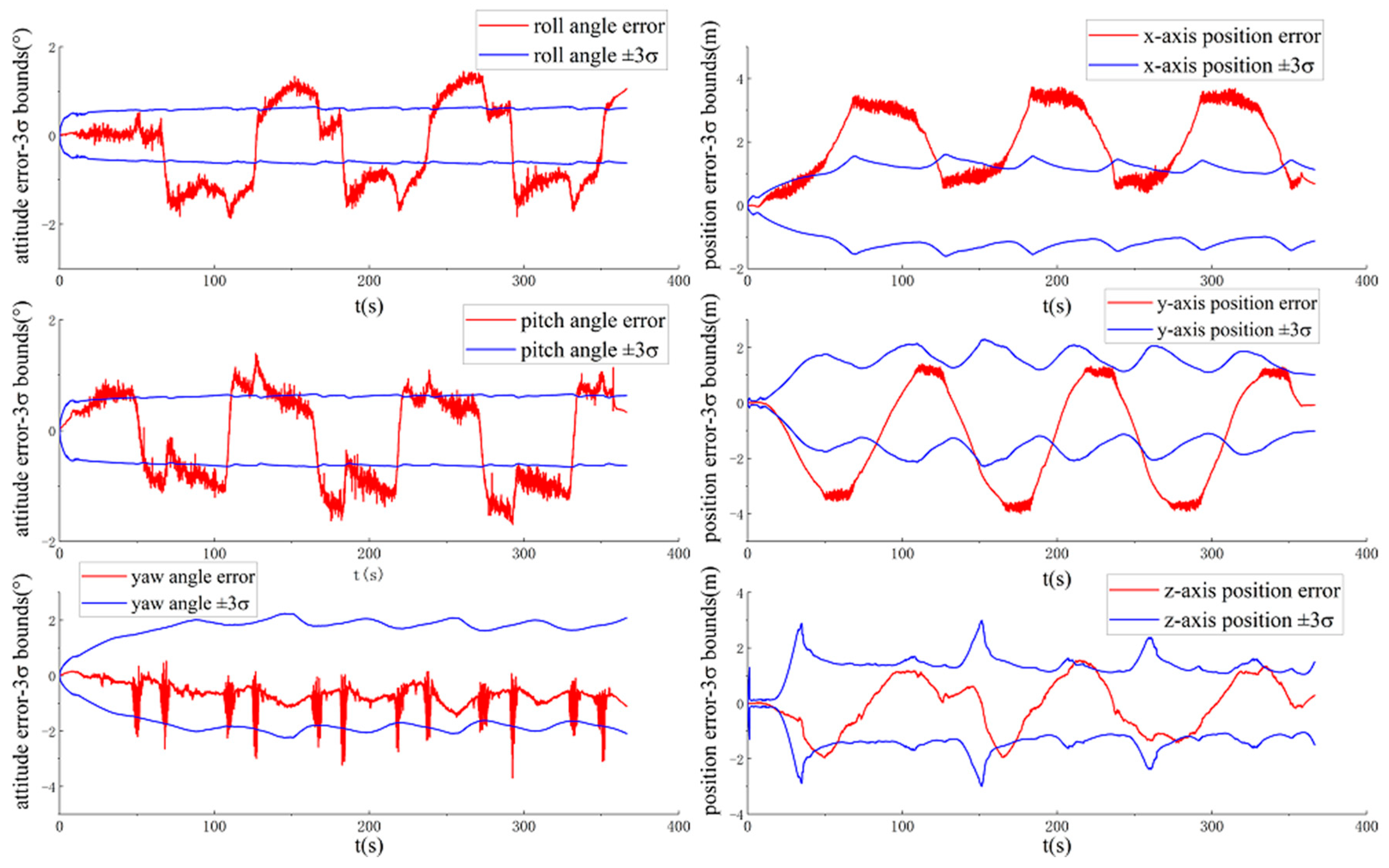
Figure 10 shows the ground-truth pose errors and estimated bounds of MAVIO-GNSS with time.
It can be seen from Figure 10 that the three-axis vehicle position error state and yaw angle error state of MAVIO-GNSS are observable, which benefits from the raw GNSS error measurement model. This implies that MAVIO-GNSS can obtain a global position for a vehicle under a long-distance driving state.
By averaging all rounds of experimental results, the better performance of the RMSSR among the different configurations at the last time step for each experimental dataset is shown in Table 4.
It can be seen from the quantitative results in Table 4 that the average RMSSRs of MAVIO and ACK-MSCKF are smaller than the RMSSR for S-MSCKF for all of the datasets. Taken together, the above results indicate that both MAVIO and ACK-MSCKF can improve the observability of the VIO scale direction.
3.2.2. Positioning Accuracy Comparison
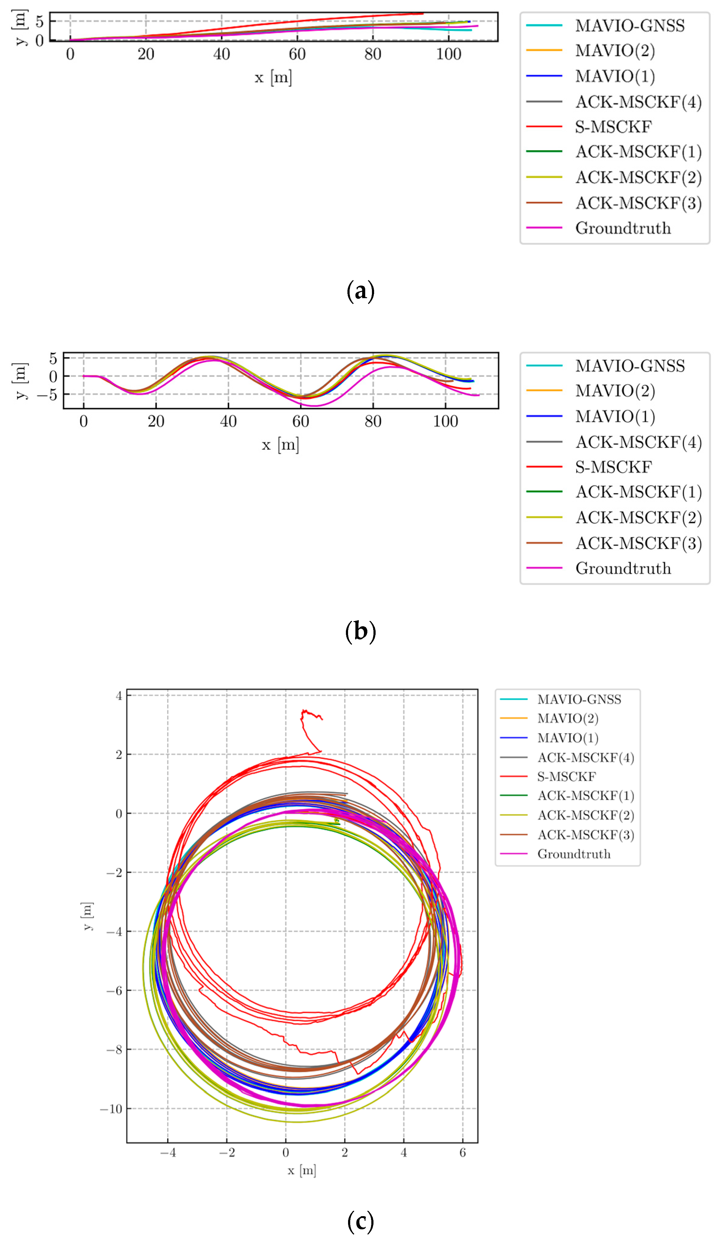
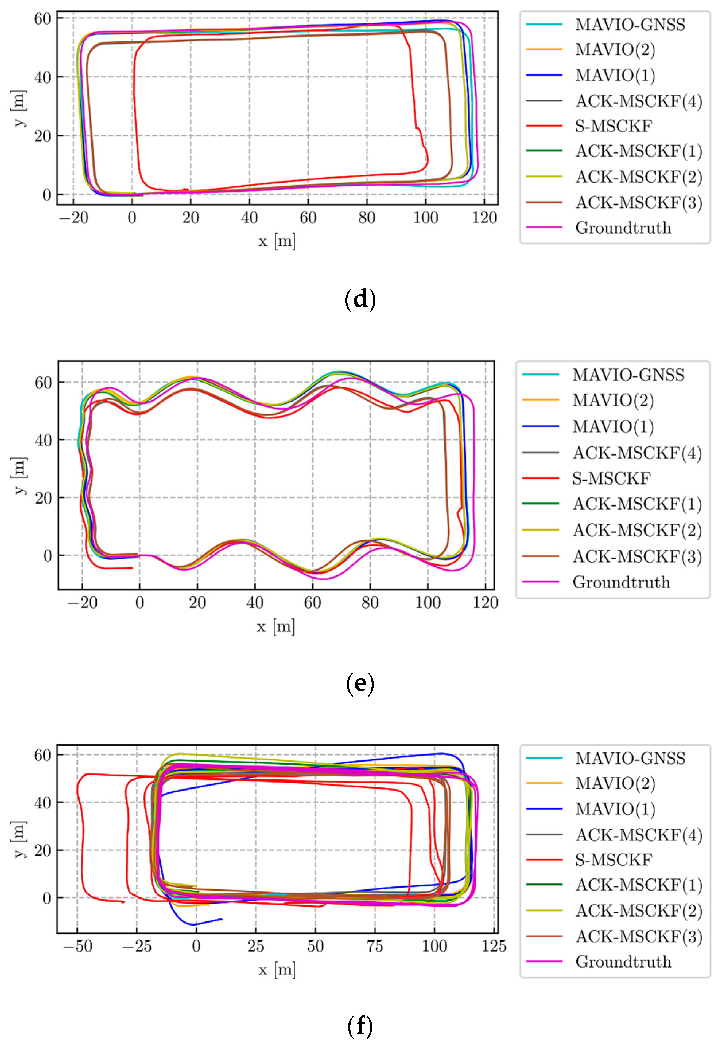
Figure 11 shows the vehicle trajectory estimation results with a top view.
Figure 11 shows that S-MSCKF has larger scale drift, especially for the VD01, VD03, VD04 and VD06 datasets. Meanwhile, by selecting the appropriate parameter configuration in practice, the estimated trajectories of ACK-MSCKF and proposed MAVIO align to the ground truth better than S-MSCKF for all of the datasets. The performance difference among the different parameter configurations of ACK-MSCKF could be attributed to the inconsistency problem mentioned above. By improving the consistency, MAVIO is more robust than ACK-MSCKF. By introducing the raw GNSS error measurements, MAVIO-GNSS performs better than MAVIO, especially for the long-distance VD06 dataset.
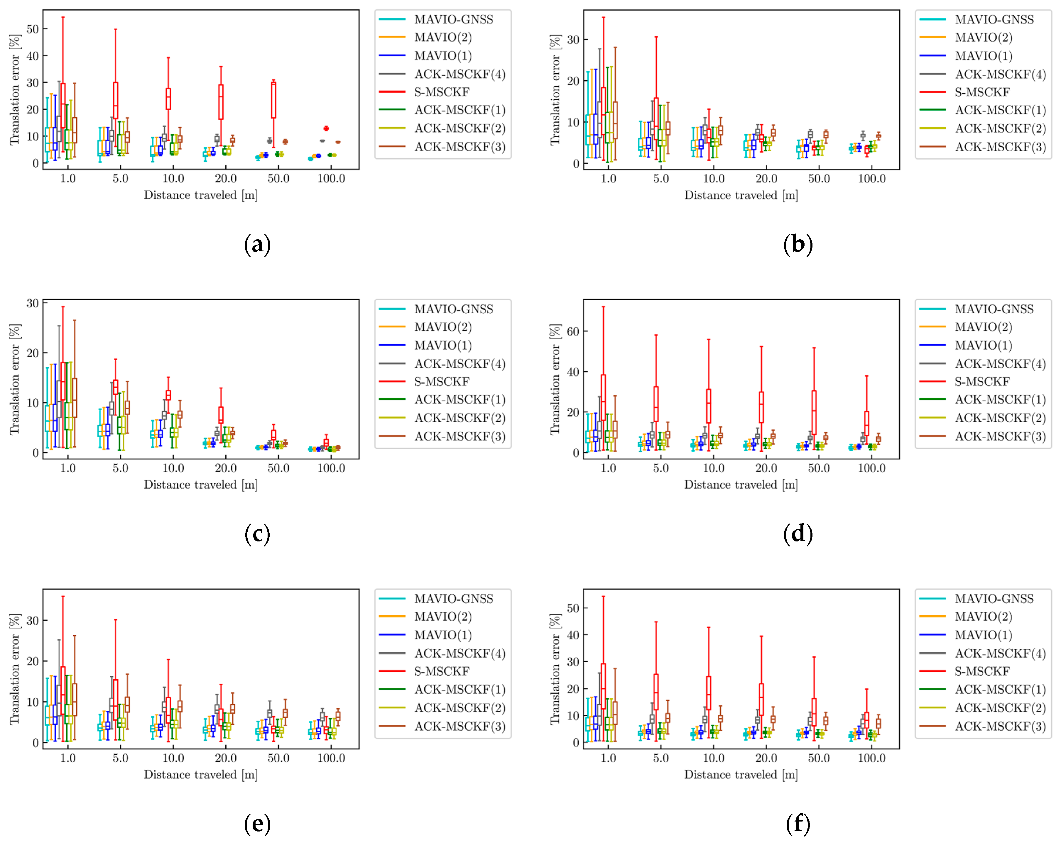
The boxplots of the RTEPs are shown in Figure 12.
Figure 12 demonstrates that the RTEPs of ACK-MSCKF and the proposed MAVIO are significantly reduced in comparison to the RTEP of S-MSCKF within the sub-trajectory length of 5 m for all of the datasets. Based on the average results for twenty rounds of experiments, the better performance of ATE among the different configurations along the whole trajectory for each experimental dataset is shown in Table 5, and Table 6 shows the overall RTE for all of the experimental datasets.
The quantitative results in Table 5 show that the average ATEs of MAVIO, MAVIO-GNSS and ACK-MSCKF is smaller than the ATE of S-MSCKF for all of the datasets but VD02. The trajectory error difference of S-MSCKF with that in [48] for the VD05 dataset is attributed to the data average processing which ensures more generalizable result. Compared with S-MSCKF, MAVIO reduces the average ATE by 86.61%, 68.03%, 86.45%, 25.65% and 78.26% for the VD01, VD03, VD04, VD05 and VD06 datasets, respectively. Moreover, MAVIO performs better than ACK-MSCKF for the VD01, VD02, VD03, VD04 and VD05 datasets, which reduces the average ATEs by 18.13%, 4.67%, 10.34%, 18.29% and 13.90%, respectively. It is also observable that MAVIO performs worse than ACK-MSCKF for the VD06 dataset. A potential reason is that the extrinsic parameters between {B} and {I} are not accurate enough. Furthermore, MAVIO-GNSS performs better than MAVIO for the VD01, VD02, VD04 and VD06 datasets, which reduces the average ATEs by 6.87%, 7.35%, 16.92% and 30.66%, respectively.
Table 6 shows that the overall RTE of MAVIO within the sub-trajectory length of 20 m is smaller than that of ACK-MSCKF. MAVIO-GNSS performs best in terms of the RTE within the sub-trajectory length of 100 m. The lowest RTE from MAVIO-GNSS is 2.29 m in the sub-trajectory length of 100 m, which is reduced, respectively, by 17.92%, 10.89% and 72.51% under the same conditions compared to that with MAVIO, ACK-MSCKF and S-MSCKF.
4. Discussion
ACK-MSCKF significantly improves the observability of the VIO scale direction and positioning accuracy under degenerate motions of ground vehicles. However, for practical implementation, the appropriate parameter configuration is needed to obtain better performance due to the inconsistency problem.
By improving the observability of the VIO scale direction and overcoming the inconsistency of ACK-MSCKF, MAVIO is more robust and further improves vehicle positioning accuracy using only a monocular configuration, which mainly benefits from the vehicle velocity and yaw angular rate error measurement model instead of the relative kinematic error measurement model for the vehicle. Compared with S-MSCKF, MAVIO reduces the average ATE by 86.61%, 68.03%, 86.45%, 25.65% and 78.26% for the VD01, VD03, VD04, VD05 and VD06 datasets, respectively. Moreover, MAVIO performs better than ACK-MSCKF for the VD01, VD02, VD03, VD04 and VD05 datasets, which reduces the average ATE by 18.13%, 4.67%, 10.34%, 18.29% and 13.90%, respectively. By introducing the raw GNSS error measurement model, MAVIO-GNSS further improves the vehicle positioning accuracy under a long-distance driving state. The lowest RTE from MAVIO-GNSS is 2.29 m in the sub-trajectory length of 100 m, and it is reduced, respectively, by 17.92%, 10.89% and 72.51% under the same conditions compared to the values obtained with MAVIO, ACK-MSCKF and S-MSCKF.
5. Conclusions
This paper proposed a consistent monocular Ackermann VIO termed MAVIO. The vehicle velocity and yaw angular rate error measurement model was introduced in detail, considering the lever arm effect between {B} and {I}. To obtain a global position for the vehicle, the raw GNSS error measurement model was introduced to further improve the performance of MAVIO. The observability and positioning accuracy were comprehensively compared using real-world datasets, averaging twenty rounds of experimental results. The experimental results demonstrated that the proposed MAVIO not only improved the observability of the VIO scale direction under degenerate motions of ground vehicles, but also resolved the inconsistency problem of ACK-MSCKF to further improve the vehicle positioning accuracy. Moreover, MAVIO-GNSS further improved the vehicle positioning accuracy under a long-distance driving state.
A limitation derives from the assumptions of approximate planar motion for a low-speed driving state and highly accurate extrinsic parameters between {B} and {I}. A future research target is to further investigate the performance impact of the vehicle speed and vehicle-IMU extrinsic parameter calibration to better enhance the positioning accuracy.
Author Contributions
Conceptualization, F.M. and J.S.; funding acquisition, F.M.; investigation, S.Z.; methodology, J.S.; project administration, L.W.; resources, K.D.; supervision, F.M. and L.W.; writing—original draft, J.S.; writing—review and editing, F.M. and L.W. All authors have read and agreed to the published version of the manuscript.
Funding
This research was funded by the Jilin Province Key Technology and Development Program (Grant No. 20190302077GX).
Acknowledgments
We would like to express our gratitude for the support received from Yu Yang, and we acknowledge that some of the content of this paper refers to the dissertation [54] of J.S.
Conflicts of Interest
The authors declare no conflict of interest.
Appendix A
According to the derivation of Equation (177) in [53], is derived as
where is derived from the following formula:
According to the error quaternion representation [53], Equation (A2) is represented as
Then,
By ignoring the second order terms, Equation (A4) is represented as
Thus, Equation (A1) is represented as
Therefore, the Jacobian matrix of is represented as
Following Equation (6), is calculated as
Equation (A8) is represented as
Then,
Therefore, the Jacobian matrix of is represented as
Following Equation (6), is calculated as
Equation (A12) is represented as
Then,
Therefore, the Jacobian matrix of is represented as
According to the characteristics of the IMU noise model [53],
Equation (A16) can be represented as
Therefore,
Thereby, the analytical expressions of each block matrix in Equations (9) and (10) are derived.
Appendix B
Following Equation (7) in [48], according to the error quaternion representation [53], the Ackermann steering attitude angle error from time to time is derived as
Equation (A19) can be represented as
Then,
According to the properties of the cross product skew-symmetric matrix [53], Equation (A21) is represented as
Then,
Therefore, the measurement Jacobian matrixes of the vehicle relative rotation errors are represented as
Similarly, the velocity measurement residual at time is represented as
Then,
Equation (A26) is represented as
where
Thus, Equation (A27) is represented as
Then,
Therefore, the measurement Jacobian matrixes of the vehicle relative translation errors are represented as
Thereby, the analytical expressions of all the block matrixes in Equation (15) are derived.
Appendix C
Following Equation (16), the vehicle angular rate measurement residual at time in {B} is represented as
Based on the lever arm effect between {B} and {I}, Equation (A32) is represented as
According to the error quaternion representation [53], Equation (A33) is represented as
Therefore, the measurement Jacobian matrix of the vehicle angular rate errors is represented as
Similarly, following Equation (16), the vehicle velocity measurement residual at time in {B} is represented as
Based on the lever arm effect between {B} and {I}, Equation (A36) is represented as
According to the error quaternion representation [53], Equation (A37) is represented as
By ignoring the second order terms, Equation (A38) is represented as
Therefore, the measurement Jacobian matrix of the vehicle velocity errors is represented as
Thereby, the analytical expressions of all the block matrixes in Equation (30) are derived.
Appendix D
According to the error quaternion representation [53], Equation (31) is represented as
Following Equation (32), Equation (A41) is represented as
Therefore, the measurement Jacobian matrix of the raw GNSS errors is represented as
Thereby, the analytical expressions of all the block matrixes in Equation (34) are derived.
References
- Yang, D.; Jiang, K.; Zhao, D.; Yu, C.; Cao, Z.; Xie, S.; Xiao, Z.; Jiao, X.; Wang, S.; Zhang, K. Intelligent and connected vehicles: Current status and future perspectives. Sci. China Technol. 2018, 61, 1446–1471. [Google Scholar] [CrossRef]
- Ma, F.; Wang, J.; Yang, Y.; Wu, L.; Zhu, S.; Gelbal, S.Y.; Aksun-Guvenc, B.; Guvenc, L. Stability Design for the Homogeneous Platoon with Communication Time Delay. Automot. Innov. 2020, 3, 101–110. [Google Scholar] [CrossRef]
- Specht, M.; Specht, C.; Dąbrowski, P.; Czaplewski, K.; Smolarek, L.; Lewicka, O. Road Tests of the Positioning Accuracy of INS/GNSS Systems Based on MEMS Technology for Navigating Railway Vehicles. Energies 2020, 13, 4463. [Google Scholar] [CrossRef]
- Jiang, Q.; Wu, W.; Jiang, M.; Li, Y. A New Filtering and Smoothing Algorithm for Railway Track Surveying Based on Landmark and IMU/Odometer. Sensors 2017, 17, 1438. [Google Scholar] [CrossRef]
- Singh, K.B.; Arat, M.A.; Taheri, S. Literature review and fundamental approaches for vehicle and tire state estimation. Veh. Syst. Dyn. 2018, 57, 1643–1665. [Google Scholar] [CrossRef]
- Xiao, Z.; Yang, D.; Wen, F.; Jiang, K. A Unified Multiple-Target Positioning Framework for Intelligent Connected Vehicles. Sensors 2019, 19, 1967. [Google Scholar] [CrossRef] [Green Version]
- Ansari, K. Cooperative Position Prediction: Beyond Vehicle-to-Vehicle Relative Position–ing. IEEE Trans. Intell. Transp. Syst. 2020, 21, 1121–1130. [Google Scholar] [CrossRef]
- Lynen, S.; Achtelik, M.W.; Weiss, S.; Chli, M.; Siegwart, R. A robust and modular multi-sensor fusion approach applied to MAV navigation. In Proceedings of the 2013 IEEE/RSJ International Conference on Intelligent Robots and Systems; Institute of Electrical and Electronics Engineers (IEEE), Tokyo, Japan, 3–7 November 2013; pp. 3923–3929. [Google Scholar]
- Bloesch, M.; Omari, S.; Hutter, M.; Siegwart, R. Robust visual inertial odometry using a direct EKF-based approach. In Proceedings of the 2015 IEEE/RSJ International Conference on Intelligent Robots and Systems (IROS); Institute of Electrical and Electronics Engineers (IEEE), Hamburg, Germany, 28 September–2 October 2015; pp. 298–304. [Google Scholar]
- Mourikis, A.I.; Roumeliotis, S.I. A Multi-State Constraint Kalman Filter for Vision-aided Inertial Navigation. In Proceedings of the Proceedings 2007 ICRA. IEEE International Conference on Robotics and Automation; Institute of Electrical and Electronics Engineers (IEEE), Italy, Roma, 10–14 April 2007; pp. 3565–3572. [Google Scholar]
- Ramezani, M.; Khoshelham, K. Vehicle Positioning in GNSS-Deprived Urban Areas by Stereo Visual-Inertial Odometry. IEEE Trans. Intell. Veh. 2018, 3, 208–217. [Google Scholar] [CrossRef]
- Sun, K.; Mohta, K.; Pfrommer, B.; Watterson, M.; Liu, S.; Mulgaonkar, Y.; Taylor, C.J.; Kumar, V. Robust Stereo Visual Inertial Odometry for Fast Autonomous Flight. IEEE Robot. Autom. Lett. 2018, 3, 965–972. [Google Scholar] [CrossRef] [Green Version]
- Huai, Z.; Huang, G. Robocentric Visual-Inertial Odometry. In Proceedings of the 2018 IEEE/RSJ International Conference on Intelligent Robots and Systems (IROS); Institute of Electrical and Electronics Engineers (IEEE), Madrid, Spain, 1–5 October 2018; pp. 6319–6326. [Google Scholar]
- Geneva, P.; Eckenhoff, K.; Huang, G. A Linear-Complexity EKF for Visual-Inertial Navigation with Loop Closures. In Proceedings of the 2019 International Conference on Robotics and Automation (ICRA); Institute of Electrical and Electronics Engineers (IEEE), Montreal, QC, Canada, 20–24 May 2019; pp. 3535–3541. [Google Scholar]
- Qiu, X.; Zhang, H.; Fu, W.; Zhao, C.; Jin, Y. Monocular Visual-Inertial Odometry with an Unbiased Linear System Model and Robust Feature Tracking Front-End. Sensors 2019, 19, 1941. [Google Scholar] [CrossRef] [PubMed] [Green Version]
- Qiu, X.; Zhang, H.; Fu, W. Lightweight hybrid visual-inertial odometry with closed-form zero velocity update. Chin. J. Aeronaut. 2020. [Google Scholar] [CrossRef]
- Leutenegger, S.; Lynen, S.; Bosse, M.; Siegwart, R.; Furgale, P. Keyframe-based visual–inertial odometry using nonlinear optimization. Int. J. Robot. Res. 2014, 34, 314–334. [Google Scholar] [CrossRef] [Green Version]
- Mur-Artal, R.; Tardos, J.D. Visual-Inertial Monocular SLAM With Map Reuse. IEEE Robot. Autom. Lett. 2017, 2, 796–803. [Google Scholar] [CrossRef] [Green Version]
- Qin, T.; Li, P.; Shen, S. VINS-Mono: A Robust and Versatile Monocular Visual-Inertial State Estimator. IEEE Trans. Robot. 2018, 34, 1004–1020. [Google Scholar] [CrossRef] [Green Version]
- He, Y.; Zhao, J.; Guo, Y.; He, W.; Yuan, K. PL-VIO: Tightly-Coupled Monocular Visual–Inertial Odometry Using Point and Line Features. Sensors 2018, 18, 1159. [Google Scholar] [CrossRef] [PubMed] [Green Version]
- Liu, H.; Chen, M.; Zhang, G.; Bao, H.; Bao, Y. ICE-BA: Incremental, Consistent and Efficient Bundle Adjustment for Visual-Inertial SLAM. In Proceedings of the IEEE Conference on Computer Vision and Pattern Recognition(CVPR), Salt Lake City, UT, USA, 18–23 June 2018; pp. 1974–1982. [Google Scholar]
- Von Stumberg, L.; Usenko, V.; Cremers, D. Direct Sparse Visual-Inertial Odometry Using Dynamic Marginalization. In Proceedings of the 2018 IEEE International Conference on Robotics and Automation (ICRA); Institute of Electrical and Electronics Engineers (IEEE), Brisbane Convention & Exhibition Centre, Brisbane, Australia, 21–25 May 2018; pp. 2510–2517. [Google Scholar]
- Qin, T.; Cao, S.; Pan, J.; Shen, S. A General Optimization-based Framework for Global Pose Estimation with Multiple Sensors. Available online: https://arxiv.org/abs/1901.03642 (accessed on 11 July 2020).
- Qin, T.; Pan, J.; Cao, S.; Shen, S. A General Optimization-based Framework for Local Odometry Estimation with Multiple Sensors. Available online: https://arxiv.org/abs/1901.03638 (accessed on 11 July 2020).
- Usenko, V.; Demmel, N.; Schubert, D.; Stueckler, J.; Cremers, D. Visual-Inertial Mapping With Non-Linear Factor Recovery. IEEE Robot. Autom. Lett. 2020, 5, 422–429. [Google Scholar] [CrossRef] [Green Version]
- Campos, C.; Elvira, R.; Rodríguez, J.J.G.; Montiel, J.M.M.; Tardós, J.D. ORB-SLAM3: An Accurate Open-Source Library for Visual, Visual-Inertial and Multi-Map SLAM. Available online: https://arxiv.org/abs/2007.11898 (accessed on 24 July 2020).
- Scaramuzza, D.; Zhang, Z. Visual-Inertial Odometry of Aerial Robots. Available online: https://arxiv.org/abs/1906.03289 (accessed on 11 July 2020).
- Huang, G. Visual-Inertial Navigation: A Concise Review. In Proceedings of the 2019 International Conference on Robotics and Automation (ICRA); Institute of Electrical and Electronics Engineers (IEEE), Montreal, QC, Canada, 20–24 May 2019; pp. 9572–9582. [Google Scholar]
- Wu, K.J.; Roumeliotis, S.I. Unobservable Directions of VINS under Special Motions; University of Minnesota: Minneapolis, MN, USA, September 2016; Available online: http://mars.cs.umn.edu/research/VINSodometry.php (accessed on 1 September 2019).
- Wu, K.J.; Guo, C.X.; Georgiou, G.; Roumeliotis, S.I. VINS on wheels. In Proceedings of the 2017 IEEE International Conference on Robotics and Automation (ICRA); Institute of Electrical and Electronics Engineers (IEEE), Singapore, 29 May–3 June 2017; pp. 5155–5162. [Google Scholar]
- Yang, Y.; Geneva, P.; Eckenhoff, K.; Huang, G. Degenerate Motion Analysis for Aided INS With Online Spatial and Temporal Sensor Calibration. IEEE Robot. Autom. Lett. 2019, 4, 2070–2077. [Google Scholar] [CrossRef]
- Wu, K.; Ahmed, A.; Georgiou, G.; Roumeliotis, S. A Square Root Inverse Filter for Efficient Vision-aided Inertial Navigation on Mobile Devices. In Proceedings of the Robotics: Science and Systems XI, Science and Systems Foundation, Rome, Italy, 13–17 July 2015. [Google Scholar]
- Li, D.; Eckenhoff, K.; Wu, K.; Wang, Y.; Xiong, R.; Huang, G. Gyro-aided camera-odometer online calibration and localization. In Proceedings of the 2017 American Control Conference (ACC); Institute of Electrical and Electronics Engineers (IEEE), Seattle, WA, USA, 24–26 May 2017; pp. 3579–3586. [Google Scholar]
- Mur-Artal, R.; Montiel, J.M.M.; Tardos, J.D. ORB-SLAM: A Versatile and Accurate Monocular SLAM System. IEEE Trans. Robot. 2015, 31, 1147–1163. [Google Scholar] [CrossRef] [Green Version]
- Mur-Artal, R.; Tardos, J.D. ORB-SLAM2: An Open-Source SLAM System for Monocular, Stereo, and RGB-D Cameras. IEEE Trans. Robot. 2017, 33, 1255–1262. [Google Scholar] [CrossRef] [Green Version]
- Houseago, C.; Bloesch, M.; Leutenegger, S. KO-Fusion: Dense Visual SLAM with Tightly-Coupled Kinematic and Odometric Tracking. In Proceedings of the 2019 International Conference on Robotics and Automation (ICRA); Institute of Electrical and Electronics Engineers (IEEE), Montreal, QC, Canada, 20–24 May 2019; pp. 4054–4060. [Google Scholar]
- Zheng, F.; Liu, Y.-H. SE(2)-Constrained Visual Inertial Fusion for Ground Vehicles. IEEE Sensors J. 2018, 18, 9699–9707. [Google Scholar] [CrossRef]
- Dang, Z.; Wang, T.; Pang, F. Tightly-coupled Data Fusion of VINS and Odometer Based on Wheel Slip Estimation. In Proceedings of the 2018 IEEE International Conference on Robotics and Biomimetics (ROBIO); Institute of Electrical and Electronics Engineers (IEEE), Kuala Lumpur, Malaysia, 12–15 December 2018; pp. 1613–1619. [Google Scholar]
- Quan, M.; Piao, S.; Tan, M.; Huang, S.-S. Tightly-Coupled Monocular Visual-Odometric SLAM Using Wheels and a MEMS Gyroscope. IEEE Access 2019, 7, 97374–97389. [Google Scholar] [CrossRef]
- Liu, J.; Gao, W.; Hu, Z. Visual-Inertial Odometry Tightly Coupled with Wheel Encoder Adopting Robust Initialization and Online Extrinsic Calibration. In Proceedings of the 2019 IEEE/RSJ International Conference on Intelligent Robots and Systems (IROS); Institute of Electrical and Electronics Engineers (IEEE), Macau, China, 4–8 November 2019; pp. 5391–5397. [Google Scholar]
- Liu, J.; Gao, W.; Hu, Z. Bidirectional Trajectory Computation for Odometer-Aided Visual-Inertial SLAM. Available online: https://arxiv.org/abs/2002.00195 (accessed on 2 February 2020).
- Zhang, M.; Chen, Y.; Li, M. Vision-Aided Localization For Ground Robots. In Proceedings of the 2019 IEEE/RSJ International Conference on Intelligent Robots and Systems (IROS); Institute of Electrical and Electronics Engineers (IEEE), Macau, China, 4–8 November 2019; pp. 2455–2461. [Google Scholar]
- Ye, W.; Zheng, R.; Zhang, F.; Ouyang, Z.; Liu, Y. Robust and Efficient Vehicles Motion Estimation with Low-Cost Multi-Camera and Odometer-Gyroscope. In Proceedings of the 2019 IEEE/RSJ International Conference on Intelligent Robots and Systems (IROS); Institute of Electrical and Electronics Engineers (IEEE), Macau, China, 4–8 November 2019; pp. 4490–4496. [Google Scholar]
- Gang, P.; Zezao, L.; Bocheng, C.; Shanliang, C.; Dingxin, H. Robust Tightly-Coupled Pose Estimation Based on Monocular Vision, Inertia and Wheel Speed. Available online: https://arxiv.org/abs/2003.01496 (accessed on 11 July 2020).
- Zuo, X.; Zhang, M.; Chen, Y.; Liu, Y.; Huang, G.; Li, M. Visual-Inertial Localization for Skid-Steering Robots with Kinematic Constraints. Available online: https://arxiv.org/abs/1911.05787 (accessed on 11 July 2020).
- Kang, R.; Xiong, L.; Xu, M.; Zhao, J.; Zhang, P. VINS-Vehicle: A Tightly-Coupled Vehicle Dynamics Extension to Visual-Inertial State Estimator. In Proceedings of the 2019 IEEE Intelligent Transportation Systems Conference (ITSC); Institute of Electrical and Electronics Engineers (IEEE), Auckland, New Zealand, 27–30 October 2019; pp. 3593–3600. [Google Scholar]
- Lee, W.; Eckenhoff, K.; Yang, Y.; Geneva, P.; Huang, G. Visual-Inertial-Wheel Odometry with Online Calibration. In Proceedings of the 2020 International Conference on Intelligent Robots and Systems (IROS), Las Vegas, NV, USA, 24–30 October 2020. [Google Scholar]
- Ma, F.; Shi, J.; Yang, Y.; Li, J.; Dai, K. ACK-MSCKF: Tightly-Coupled Ackermann Multi-State Constraint Kalman Filter for Autonomous Vehicle Localization. Sensors 2019, 19, 4816. [Google Scholar] [CrossRef] [Green Version]
- Lee, W.; Eckenhoff, K.; Geneva, P.; Huang, G. Intermittent GPS-aided VIO: Online Initialization and Calibration. In Proceedings of the 2020 IEEE International Conference on Robotics and Automation (ICRA); Institute of Electrical and Electronics Engineers (IEEE), Paris, France, 31 May–31 August 2020; pp. 5724–5731. [Google Scholar]
- MAVIO ROS Package. Available online: https://github.com/qdensh/MAVIO (accessed on 12 August 2020).
- Grafarend, E. The Optimal Universal Transverse Mercator Projection. In International Association of Geodesy Symposia; Springer Science and Business Media LLC: Berlin/Heidelberg, Germany, 1995; Volume 114, p. 51. [Google Scholar]
- Breckenridge, W.G. Quaternions proposed standard conventions. Jet Propuls. Lab. Pasadena, CA, Interoffice Memo. IOM 1999, 343–379. [Google Scholar]
- Trawny, N.; Roumeliotis, S.I. Indirect Kalman Filter for 3D Attitude Estimation; University of Minnesota: Minnesota, MN, USA, 2005; Volume 2, p. 2005. [Google Scholar]
- Shi, J. Visual-Inertial Pose Estimation and Observability Analysis with Vehicle Motion Constraints. Ph.D. dissertation, Jilin University, Changchun, China, June 2020. (In Chinese). [Google Scholar]
- Kevin, M.L.; Park, F.C. Modern Robotics: Mechanics, Planning, and Control, 1st ed.; Cambridge University Press: New York, NY, USA, 2017. [Google Scholar]
- Robot_Localization ROS Package. Available online: https://github.com/cra-ros-pkg/robot_localization (accessed on 1 June 2019).
- Markley, F.L.; Cheng, Y.; Crassidis, J.L.; Oshman, Y. Averaging Quaternions. J. Guid. Control. Dyn. 2007, 30, 1193–1197. [Google Scholar] [CrossRef]
- Zhang, Z.; Scaramuzza, D. A Tutorial on Quantitative Trajectory Evaluation for Visual(-Inertial) Odometry. In Proceedings of the 2018 IEEE/RSJ International Conference on Intelligent Robots and Systems (IROS); Institute of Electrical and Electronics Engineers (IEEE), Madrid, Spain, 1–5 October 2018; pp. 7244–7251. [Google Scholar]
- AverageVioProc ROS Package. Available online: https://github.com/qdensh/AverageVioProc (accessed on 12 August 2020).
- Hesch, J.A.; Kottas, D.G.; Bowman, S.L.; Roumeliotis, S.I. Consistency Analysis and Improvement of Vision-aided Inertial Navigation. IEEE Trans. Robot. 2013, 30, 158–176. [Google Scholar] [CrossRef] [Green Version]
- Umeyama, S. Least-squares estimation of transformation parameters between two point patterns. IEEE Trans. Pattern Anal. Mach. Intell. 1991, 13, 376–380. [Google Scholar] [CrossRef] [Green Version]
- Msckf_Vio_GPS Package. Available online: https://github.com/ZhouTangtang/msckf_vio_GPS (accessed on 11 July 2019).
- Kalibr_Allan ROS Package. Available online: https://github.com/rpng/kalibr_allan (accessed on 14 February 2019).
- Hesch, J.A.; Kottas, D.G.; Bowman, S.L.; Roumeliotis, S.I. Observability-Constrained Vision-Aided Inertial Navigation; University of Minnesota: Minneapolis, MN, USA, 2012; Volume 1, p. 6. [Google Scholar]
Figure 1.
The lever arm effect between {B} and {I}. denotes the rotation quaternion from {GI} to {I} at time ; denotes the position of {I} in {GI} at time . denotes the rotation quaternion from {GI} to {B} at time ; denotes the position of {B} in {GI} at time . and denote the rotation and translation extrinsic parameters between {B} and {I} at time , respectively. denotes the velocity of {I} in {GI} at time ; denotes the vehicle velocity at time . and denote the angular rates of {I} and {B} at time , respectively.

Figure 2.
Experimental vehicle platform: Vehicle_a27.

Figure 3.
The ground-truth vehicle longitudinal speeds for the datasets: (a) VD01; (b) VD02; (c) VD03; (d) VD04; (e) VD05; (f) VD06.
Figure 3.
The ground-truth vehicle longitudinal speeds for the datasets: (a) VD01; (b) VD02; (c) VD03; (d) VD04; (e) VD05; (f) VD06.
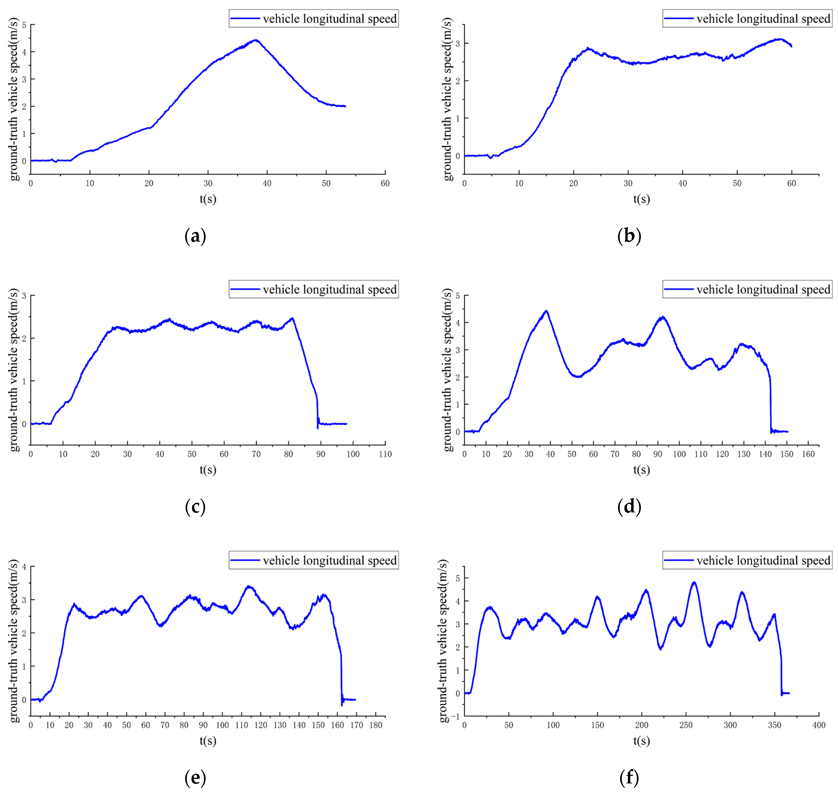
Figure 4.
The ground-truth pose errors and estimated bounds of ACK-MSCKF(1) with time for the VD06 dataset.
Figure 4.
The ground-truth pose errors and estimated bounds of ACK-MSCKF(1) with time for the VD06 dataset.

Figure 5.
The ground-truth pose errors and estimated bounds of ACK-MSCKF(2) with time for the VD06 dataset.
Figure 5.
The ground-truth pose errors and estimated bounds of ACK-MSCKF(2) with time for the VD06 dataset.

Figure 6.
The ground-truth pose errors and estimated bounds of ACK-MSCKF(3) with time for the VD06 dataset.
Figure 6.
The ground-truth pose errors and estimated bounds of ACK-MSCKF(3) with time for the VD06 dataset.
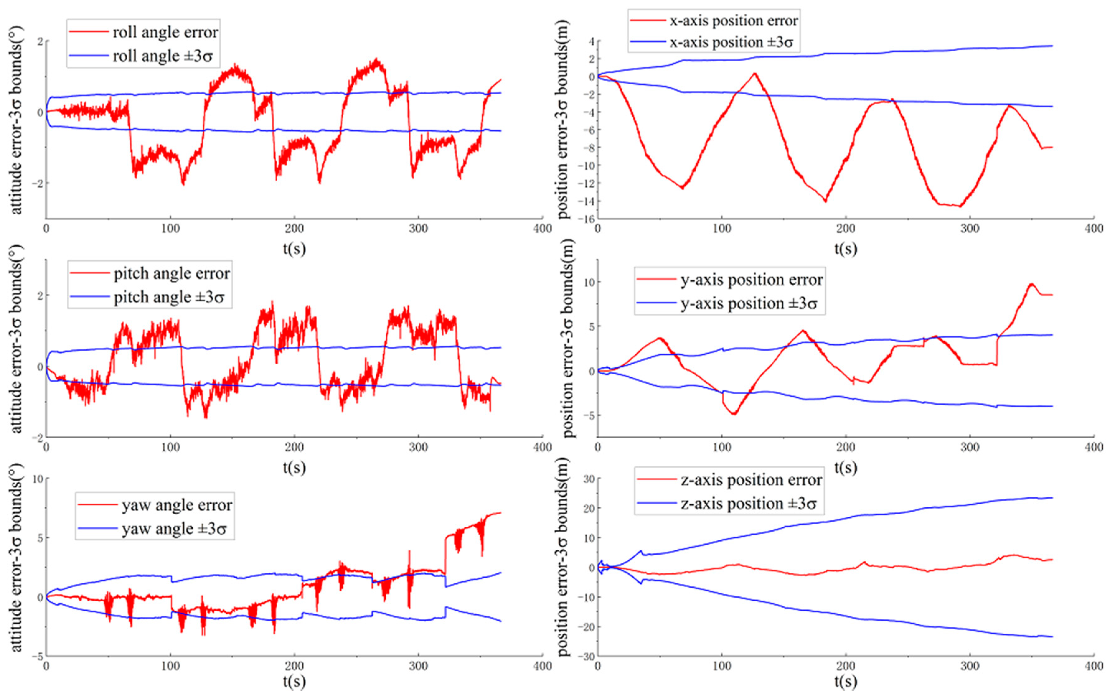
Figure 7.
The ground-truth pose errors and estimated bounds of ACK-MSCKF(4) with time for the VD06 dataset.
Figure 7.
The ground-truth pose errors and estimated bounds of ACK-MSCKF(4) with time for the VD06 dataset.

Figure 8.
The ground-truth pose errors and estimated bounds of MAVIO(1) with time for the VD06 dataset.
Figure 8.
The ground-truth pose errors and estimated bounds of MAVIO(1) with time for the VD06 dataset.

Figure 9.
The ground-truth pose errors and estimated bounds of MAVIO(2) with time for the VD06 dataset.
Figure 9.
The ground-truth pose errors and estimated bounds of MAVIO(2) with time for the VD06 dataset.

Figure 10.
The ground-truth pose errors and estimated bounds of the MAVIO-Global Navigation Satellite System (GNSS) with time for the VD06 dataset.
Figure 10.
The ground-truth pose errors and estimated bounds of the MAVIO-Global Navigation Satellite System (GNSS) with time for the VD06 dataset.

Figure 11.
The top-views of estimated trajectories from MAVIO, MAVIO-GNSS, ACK-MSCKF, S-MSCKF and Groundtruth for the datasets: (a) VD01; (b) VD02; (c) VD03; (d) VD04; (e) VD05; (f) VD06.
Figure 11.
The top-views of estimated trajectories from MAVIO, MAVIO-GNSS, ACK-MSCKF, S-MSCKF and Groundtruth for the datasets: (a) VD01; (b) VD02; (c) VD03; (d) VD04; (e) VD05; (f) VD06.


Figure 12.
The relative translation error percentages (RTEPs) for MAVIO, MAVIO-GNSS, ACK-MSCKF and S-MSCKF for the datasets: (a) VD01; (b) VD02; (c) VD03; (d) VD04; (e) VD05; (f) VD06.
Figure 12.
The relative translation error percentages (RTEPs) for MAVIO, MAVIO-GNSS, ACK-MSCKF and S-MSCKF for the datasets: (a) VD01; (b) VD02; (c) VD03; (d) VD04; (e) VD05; (f) VD06.


Table 1.
The tunable parameter configurations of ACK-MSCKF.
| ACK-MSCKF | Tunable Parameter Configurations |
|---|---|
| ACK-MSCKF(1) | For Equations (A24) and (A31), |
| ACK-MSCKF(2) | For Equations (A24) and (A31), |
| ACK-MSCKF(3) | Same as Equations (A24) and (A31) |
| ACK-MSCKF(4) | For Equation (A24), |
Table 2.
The tunable parameter configurations of the monocular Ackermann visual–inertial odometry (VIO) (MAVIO).
Table 2.
The tunable parameter configurations of the monocular Ackermann visual–inertial odometry (VIO) (MAVIO).
| MAVIO | Tunable Parameter Configurations |
|---|---|
| MAVIO(1) | Same as Equations (A35) and (A40) |
| MAVIO(2) | For Equation (A35), |
Table 3.
List of the real-world experimental datasets adapted from [54].
Table 3.
List of the real-world experimental datasets adapted from [54].
| Dataset | Vehicle Driving State | Travel Duration (s) | Travel Distance (m) | Data Bulk | |||
|---|---|---|---|---|---|---|---|
| Vehicle CAN-Bus | Stereo Images | IMU | Ground Truth | ||||
| VD01 | Straight | 54 | 109 | 8657 | 1615 | 10,808 | 10,818 |
| VD02 | S-shaped | 60 | 122 | 9644 | 1820 | 12,146 | 12,186 |
| VD03 | Circular | 99 | 162 | 15,631 | 2959 | 19,716 | 19,789 |
| VD04 | Straight and Turning | 151 | 371 | 24,171 | 4532 | 30,164 | 30,244 |
| VD05 | S-shaped and Straight and Turning | 170 | 400 | 27,135 | 5102 | 33,933 | 34,025 |
| VD06 | Straight and Turning | 367 | 1085 | 58,463 | 11,014 | 73,169 | 73,386 |
Table 4.
The average root mean square scale ratio (RMSSR) at the last time step on each experimental dataset.
Table 4.
The average root mean square scale ratio (RMSSR) at the last time step on each experimental dataset.
| Methods | VD01 | VD02 | VD03 | VD04 | VD05 | VD06 |
|---|---|---|---|---|---|---|
| MAVIO | 1.29 (a) | 1.29 (a,b) | 1.14 (b) | 1.42 (a) | 1.42 (b) | 1.63 (a) |
| ACK-MSCKF | 1.21 (f) | 1.11 (f) | 0.98 (d,e,f) | 1.31 (f) | 1.21 (f) | 1.46 (f) |
| S-MSCKF | 1.68 | 1.38 | 1.22 | 1.99 | 1.57 | 2.08 |
(a) From MAVIO(1); (b) From MAVIO(2); (c) From ACK-MSCKF(1); (d) From ACK-MSCKF(2); (e) From ACK-MSCKF(3); (f) From ACK-MSCKF(4).
Table 5.
The average absolute trajectory error (ATE) along the whole trajectory for each experimental dataset.
Table 5.
The average absolute trajectory error (ATE) along the whole trajectory for each experimental dataset.
| Methods | VD01 (m) | VD02 (m) | VD03 (m) | VD04 (m) | VD05 (m) | VD06 (m) |
|---|---|---|---|---|---|---|
| MAVIO | 1.31 (b) | 2.45 (b) | 0.78 (a) | 2.01 (b) | 3.16 (b) | 4.73 (b) |
| MAVIO-GNSS | 1.22 | 2.27 | 0.79 | 1.67 | 3.59 | 3.28 |
| ACK-MSCKF | 1.60 (d) | 2.57 (c) | 0.87 (d) | 2.46 (c,d) | 3.67 (d) | 3.80 (d) |
| S-MSCKF | 9.78 | 2.31 | 2.44 | 14.83 | 4.25 | 21.76 |
(a) From MAVIO(1); (b) From MAVIO(2); (c) From ACK-MSCKF(1); (d) From ACK-MSCKF(2); (e) From ACK-MSCKF(3); (f) From ACK-MSCKF(4).
Table 6.
The overall relative translation error (RTE) for all of the experimental datasets.
| Sub-Trajectory Length (m) | Relative Translation Error (m) | |||
|---|---|---|---|---|
| MAVIO | MAVIO-GNSS | ACK-MSCKF | S-MSCKF | |
| 1 | 0.08 (a, b) | 0.08 | 0.08 (c, d) | 0.22 |
| 5 | 0.23 (b) | 0.21 | 0.26 (c, d) | 0.93 |
| 10 | 0.40 (b) | 0.35 | 0.44 (c, d) | 1.71 |
| 20 | 0.70 (b) | 0.60 | 0.76 (d) | 3.00 |
| 50 | 1.51 (b) | 1.29 | 1.51 (d) | 5.57 |
| 100 | 2.79 (b) | 2.29 | 2.57 (d) | 8.33 |
(a) From MAVIO(1); (b) From MAVIO(2); (c) From ACK-MSCKF(1); (d) From ACK-MSCKF(2); (e) From ACK-MSCKF(3); (f) From ACK-MSCKF(4).
© 2020 by the authors. Licensee MDPI, Basel, Switzerland. This article is an open access article distributed under the terms and conditions of the Creative Commons Attribution (CC BY) license (http://creativecommons.org/licenses/by/4.0/).
Share and Cite
MDPI and ACS Style
Ma, F.; Shi, J.; Wu, L.; Dai, K.; Zhong, S. Consistent Monocular Ackermann Visual–Inertial Odometry for Intelligent and Connected Vehicle Localization. Sensors 2020, 20, 5757. https://doi.org/10.3390/s20205757
AMA Style
Ma F, Shi J, Wu L, Dai K, Zhong S. Consistent Monocular Ackermann Visual–Inertial Odometry for Intelligent and Connected Vehicle Localization. Sensors. 2020; 20(20):5757. https://doi.org/10.3390/s20205757
Chicago/Turabian StyleMa, Fangwu, Jinzhu Shi, Liang Wu, Kai Dai, and Shouren Zhong. 2020. "Consistent Monocular Ackermann Visual–Inertial Odometry for Intelligent and Connected Vehicle Localization" Sensors 20, no. 20: 5757. https://doi.org/10.3390/s20205757
Note that from the first issue of 2016, this journal uses article numbers instead of page numbers. See further details here.