Local Stability Analysis for a Thermo-Economic Irreversible Heat Engine Model under Different Performance Regimes

Abstract

A recent work reported a local stability analysis of a thermo-economical model of an irreversible heat engine working under maximum power conditions. That work showed that after small perturbations to the working temperatures, the system decreases exponentially to the steady state characterized by two different relaxation times. This work extends the local stability analysis considering other performance regimes: the Maximum Efficient Power (MEP) and the Ecological Function (EF) regimes. The relaxation time was shown under different performance regimes as functions of the temperature ratio $\mathsf{\tau }=T_2/T_1$, with $T_1>T_2$, the fractional fuel cost f and a lumped parameter R related to the internal irreversibilities degree. Under Maximum Efficient Power conditions the relaxation times are less than the relaxation times under both Maximum Ecological function and Maximum Power. At Maximum Power Efficient conditions, the model gives better stability conditions than for the other two regimes.

1. Introduction

In 2001, Santillán et al. [1] studied the local stability analysis of an endoreversible Curzon-Ahlborn heat engine [2] operating under maximum power conditions. Later, Guzmán-Vargas et al. [3] investigated the effect of the heat transfer laws and the thermal conductances on the local stability of an endoreversible heat engine. Recently, Páez-Hernández et al. [4], analyzed the local stability of a non-endoreversible Curzon-Ahlborn (CA) cycle taking into account implicity the engine’s time delays operating under maximum power regime. However, the local stability analysis described in these works have not considered economical effects. Within the context of Finite-Time Thermodynamics (FTT), the economical aspects were introduced earlier by De Vos [5] to study the thermo-economic model performance of a Novikov type power plant [6,7]. Later, Sahin and Kodal [8] studied the thermo-economics of an endoreversible heat engine in terms of maximization profit function defined as quotient between the power output and the annual investment and fuel consumption costs. This thermo-economic performance analysis [9] consists of maximizing a benefit function in terms of the power output and the cost involved in the power plant performance. All these thermo-economic studies have shown that the inclusion of costs of performance have an important impact in the trade off cost-benefit of the corresponding power plant models [5,10,11]. Recently, Barranco-Jiménez et al. [12,13] reported a local stability analysis of a thermo-economic model of an irreversible heat engine working under maximum power conditions. In those studies, they used two different heat transfer laws, the Newtonian [12] and the Dulong-Petit [13] ones. In this work, the local stability analysis is extended considering other performance regimes: The Maximum Efficient Power [14,15] and the Ecological Function regime [16,17]. The relaxation time shown under maximum efficient power conditions is less than the relaxation times under both maximum power and maximum ecological function; that is, under maximum efficient power conditions, there is better stability conditions than for the other two regimes. The paper is organized as follows: Section 2 presents the thermo-economic analysis of the irreversible heat engine under different performance criteria. In Section 3, the local stability analysis of the irreversible heat engine is shown. Finally, in Section 4, the conclusions are given.

2. Thermoeconomic Optimization of a Curzon-Ahlborn Engine Model at Different Regimes of  Performance

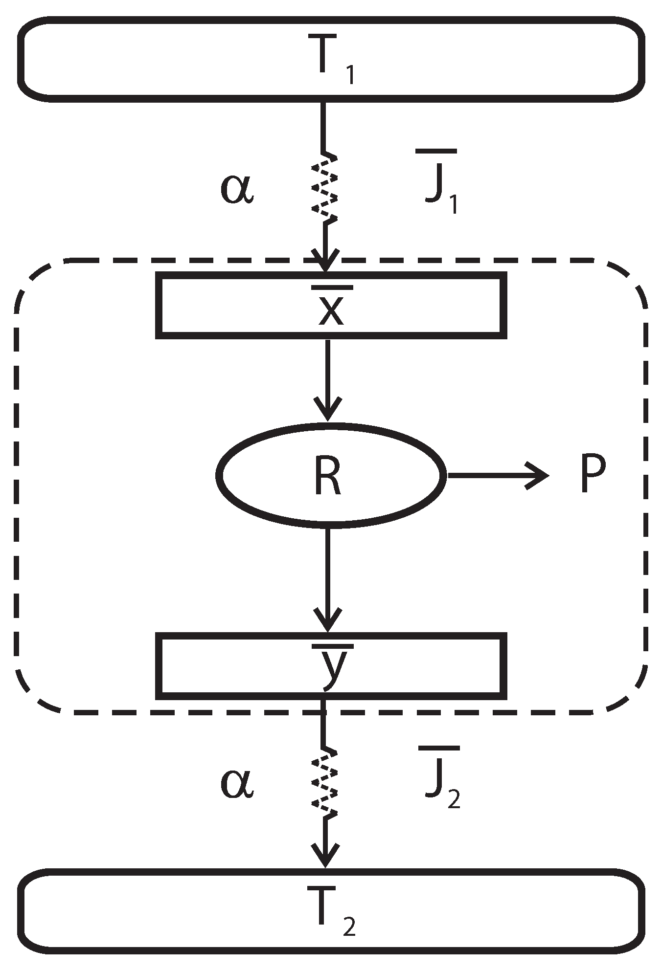
In Figure 1, a schematic diagram of the irreversible heat engine (Curzon-Ahlborn model) is shown. This engine consists of a Carnot-like thermal engine that works in irreversible cycles and exchanges heat with external thermal reservoirs at temperatures $T_1$ and $T_2$ ($T_1>T_2$). In the steady state, the temperatures of isothermals of the Carnot-like cycle are $\overline{x}$ and $\overline{y}$; here overbars are used to indicate the corresponding steady-state value. The steady-state heat flows as are shown in Figure 1 are denoted as $\overline{J_1}$ and $\overline{J_2}$, respectively.

Figure 1. Schematic representation of an endoreversible heat engine.

Figure 1. Schematic representation of an endoreversible heat engine.

Applying the Clausius theorem and using the fact that the inner Carnot-like engine works in irreversible cycles, the following inequality is obtained,

$$\frac{\overline{J_1}}{\overline{x}}-\frac{\overline{J_2}}{\overline{y}}<0,$$

(1)

this expression can be transformed into an equality by introducing a parameter R leading to,

$$\frac{\overline{J_1}}{\overline{x}}=R\frac{\overline{J_2}}{\overline{y}}.$$

(2)

The lumped parameter R, which, in principle, is within the interval $0\le R\le 1$ ($R=1$ for the endoreversible limit), can be seen as a measure of the departure from the endoreversible regime, it has been used for non endoreversible thermal heat engine models as a way to include the global internal irreversibilities [18,19]. Assuming that the heat flows from $T_1$ to $\overline{x}$ and from $\overline{y}$ to $T_2$ are of the Newton type, then

$$\overline{J_1}=\alpha (T_1-\overline{x}),$$

(3)

$$\overline{J_2}=\alpha (\overline{y}-T_2),$$

(4)

where α is the thermal conductance. For simplicity of the calculations, it is assumed that the heat exchanges take place in conductors with the same thermal conductance α; that is, the materials of both conductors are the same. Applying the first and second laws of thermodynamics, the system’s steady-state power output and the efficiency can be written as,

$$\overline{P}=\overline{J_1}-\overline{J_2},$$

(5)

and

$$\overline{\eta }=\frac{\overline{P}}{\overline{J_1}}=1-\frac{\overline{J_2}}{\overline{J_1}}=1-\frac{1}{R}\frac{\overline{y}}{\overline{x}}.$$

(6)

By combining Equations (2)–(4) and (6), gives the steady-state temperatures $\overline{x}$ and $\overline{y}$ and the power output in terms of $T_1$, $T_2$, R and $\overline{\eta }$ as [1,3],

$$\overline{x}=\frac{T_1}{1+R}\left(1+\frac{\mathsf{\tau }}{1-\overline{\eta }}\right),$$

(7)

$$\overline{y}=\frac{R}{1+R}{T}_1\left(1+\frac{\mathsf{\tau }}{1-\overline{\eta }}\right)(1-\overline{\eta }),$$

(8)

$$\overline{P}=\frac{\alpha }{1+R}{T}_1\overline{\eta }\left(R-\frac{\mathsf{\tau }}{1-\overline{\eta }}\right),$$

(9)

where $\mathsf{\tau }=T_2/T_1$. The De Vos thermoecomical analysis considers a profit function F, which is maximized [5]. This profit function is given by the quotient of the power output ($\overline{P}$) and the total cost involved in the performance of the power plant (${\overline{C}}_{tot}$), that is,

$$\overline{F}=\frac{\overline{P}}{{\overline{C}}_{tot}}.$$

(10)

In his early study, De Vos assumed that the running cost of the plant consists of two parts: a capital cost which is proportional to the investment and, therefore, to the size of the plant and, a fuel cost that is proportional to the fuel consumption and, therefore, to the heat input rate $\overline{J_1}$. Assuming that ${\overline{J}}_{max}$ is an appropriate measure for the size of the plant, the running costs of the plant exploitation are defined as [5],

$${\overline{C}}_{tot}=a{\overline{J}}_{max}+b{\overline{J}}_1=a\alpha T_1\left[(1-\mathsf{\tau })+\beta \left(1-\frac{\overline{x}}{T_1}\right)\right]$$

(11)

where the proportionality constants a and b have units of $\$/Joule$, $\beta =b/a$ and ${\overline{J}}_{max}=\alpha (T_1-T_2)$ is the maximum heat that can be extracted from the heat reservoir without supplying work (see Figure 1). By using Equations (3), (6), (7), (10) and (11), the profit function can be written as,

$$a{\overline{F}}_{MP}=\frac{\overline{\eta }\left[\frac{1}{1+R}\left(R-\frac{\mathsf{\tau }}{1-\overline{\eta }}\right)\right]}{(1-\mathsf{\tau })+\frac{\beta }{1+R}\left(R-\frac{\mathsf{\tau }}{1-\overline{\eta }}\right)}.$$

(12)

If we calculate the derivative of $a\overline{F}$ with respect to $\overline{\eta }$ and we solve for the efficiency ${\left.\frac{d\left(a{\overline{F}}_{MP}\right)}{d\overline{\eta }}\right|}_{\overline{\eta }={\overline{\eta }}^{*}}=0$, we obtain $\overline{\eta }={\overline{\eta }}^{*}(\beta ,\mathsf{\tau },R)$ [20]. However, instead of expressing the optimal efficiency in terms of the parameter β, a number that is difficult to obtain in the literature [5], we can also express it in terms of the fractional fuel cost, which is defined as [5],

$$f=\frac{\beta {\overline{J}}_1}{{\overline{J}}_{max}+\beta {\overline{J}}_1}.$$

(13)

The fractional fuel costs (f) for various technologies were reported by De Vos for different energy sources; that is, for example; renewable energy $f=0$, for Uranium $f=0.25$, for Coal $f=0.35$, and for natural gas $f=0.5$ [5]. By using Equations (3), (7) and (13), the parameter β in terms of the fractional fuel cost can be written as,

$$\beta =\frac{f}{1-f}\frac{(1+R)(1-\mathsf{\tau })}{R-\frac{\mathsf{\tau }}{1-\overline{\eta }}}.$$

(14)

Therefore, the efficiency that maximizes the profit function is given by [20],

$${\overline{\eta }}_{MP}(f,\mathsf{\tau },R)=1-\frac{f}{2R}\mathsf{\tau }-\frac{\sqrt{4(1-f)\mathsf{\tau }R+f^2{\mathsf{\tau }}^2}}{2R}.$$

(15)

Equation (15) represents the optimal steady-state efficiency ($\overline{\eta }$) as a function of τ, f and R for a non endoreversible Novikov-Curzon-Alhborn heat engine working in the maximum-power regime.

Analogously to Equation (10), for our thermo-economic optimization approach, two objective functions, the so-called Efficient Power [14,15] and the so-called Ecological Function [16,17] are defined, both divided by the total cost. The Maximum Efficient Power performance [14,15] for heat engines was studied for Yilmaz [14] and previously defined by Stucki [21] in 1980 as the product of power output (P) by the efficiency (η) in the context of the first order irreversible thermodynamics. The ecological optimization criterion for the FTT-thermal cycles was proposed by Angulo-Brown [16]. This criterion considers the maximization of a function E which represents a compromise between high power output (P) and low entropy production Σ. The E function is given by, $E=P-T_2\Sigma$ where P is the power output of the cycle, Σ the total entropy production per cycle and $T_2$ is the temperature of the cold reservoir. One of the most important characteristics of a CA engine operating under maximum-E conditions is that it produces around 80% of the maximum power and only 30% of the entropy produced in the maximum power regime [16]. Another interesting property of the maximum-E regime is that the CA-engine’s efficiency in this regime, is given by ${\eta }_E\approx ({\eta }_C+{\eta }_{CA})/2$, where ${\eta }_C$ is the Carnot efficiency and ${\eta }_{CA}$ the Curzon-Ahlborn efficiency. For our thermo-economical approach, these objective functions are given by ${\overline{F}}_{EP}=\frac{\eta \overline{P}}{{\overline{C}}_{tot}}$ and ${\overline{F}}_E=\frac{\overline{P}-T_2\Sigma }{{\overline{C}}_{tot}}$, respectively. In the same way that Equation (12) the profit functions can be written as,

$$a{\overline{F}}_{EP}=\frac{{\overline{\eta }}^2\left[\frac{1}{1+R}\left(R-\frac{\mathsf{\tau }}{1-\overline{\eta }}\right)\right]}{(1-\mathsf{\tau })+\frac{\beta }{1+R}\left(R-\frac{\mathsf{\tau }}{1-\overline{\eta }}\right)},$$

(16)

and

$$a{\overline{F}}_E=\frac{(2\overline{\eta }+\mathsf{\tau }-1)\left[\frac{1}{1+R}\left(R-\frac{\mathsf{\tau }}{1-\overline{\eta }}\right)\right]}{(1-\mathsf{\tau })+\frac{\beta }{1+R}\left(R-\frac{\mathsf{\tau }}{1-\overline{\eta }}\right)}.$$

(17)

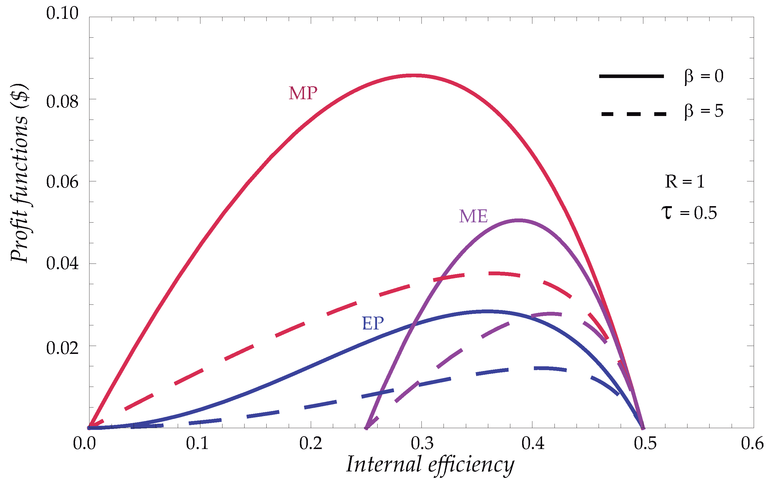
In Equation (17), the second law of thermodynamics was applied to calculate the total entropy production given by $\Sigma =\frac{{\overline{J}}_2}{T_2}-\frac{{\overline{J}}_1}{T_1}$ (see Figure 1). Figure 2 shows the behavior of the three objective functions versus internal efficiency. As can be seen from Figure 2 there exists an optimal efficiency value which depends on the parameter R, the parameter τ and the economic parameter β. In addition, Figure 2 shows for the three performance regimes how the optimal efficiency tends to the Carnot value when $\beta ⟶\infty$. Analogously to Equation (12), calculating the derivatives of $a{\overline{F}}_{EP}$ and $a{\overline{F}}_E$ with respect to $\overline{\eta }$, and solving for the efficiency the following two equations ${\left.\frac{d\left(a{\overline{F}}_{EP}\right)}{d\overline{\eta }}\right|}_{\overline{\eta }={\overline{\eta }}^{*}}=0$ and ${\left.\frac{d\left(a{\overline{F}}_E\right)}{d\overline{\eta }}\right|}_{\overline{\eta }={\overline{\eta }}^{*}}=0$ and using Equation (14) we get,

$${\overline{\eta }}_{EP}(f,\mathsf{\tau },R)=1-\frac{1+f}{4R}\mathsf{\tau }-\sqrt{\frac{(1-f)\mathsf{\tau }}{2R}+\frac{{(1+f)}^2{\mathsf{\tau }}^2}{16R^2}}.$$

(18)

$${\overline{\eta }}_E(f,\mathsf{\tau },R)=1-\frac{f}{2R}\mathsf{\tau }-\sqrt{\frac{(1-f)(1+\mathsf{\tau })\mathsf{\tau }}{2R}+\frac{f^2{\mathsf{\tau }}^2}{4R^2}}.$$

(19)

Figure 2. Profit functions for $\beta =0$ and $\beta =5$ versus η with $R=1$ and $\mathsf{\tau }=0.5$.

Figure 2. Profit functions for $\beta =0$ and $\beta =5$ versus η with $R=1$ and $\mathsf{\tau }=0.5$.

Equations (18) and (19), represent the steady-state efficiencies working both under maximum-efficient power (${\overline{\eta }}_{EP}$) and maximum ecological function conditions (${\overline{\eta }}_E$), respectively. In analogous way to Equation (15), for the endoreversible case ($R=1$) from Equations (18) and (19), when $f=0$, ($\beta =0$) we obtain $\overline{\eta }=1-\mathsf{\tau }/4-\sqrt{\mathsf{\tau }(8+\mathsf{\tau })}/4$ and $\overline{\eta }=1-\sqrt{\mathsf{\tau }(\mathsf{\tau }+1)/2}$, respectively, which were previously obtained by Yilmaz [14], and by Angulo-Brown [16,22,23], for the case of a Curzon-Ahlborn heat engine, working at maximum efficient power and maximum ecological function conditions, respectively.

We can see, in Figure 3, how the optimal efficiencies smoothly increase from the maximum efficiency point, $f=0$ (in each regime of operation), corresponding to energy sources where the investment is the preponderant cost up to the Carnot value for $f=1$, that is, for energy sources where the fuel is the predominant cost [5], and we can also observe that the following inequality, ${\overline{\eta }}_E>{\overline{\eta }}_{EP}>{\overline{\eta }}_{MP}$ is hold [10,11].

Figure 3. The steady-state efficiencies working under maximum power output (${\overline{\eta }}_{MP}$), maximum-efficient power (${\overline{\eta }}_{EP}$) and maximum ecological function (${\overline{\eta }}_E$) conditions.

Figure 3. The steady-state efficiencies working under maximum power output (${\overline{\eta }}_{MP}$), maximum-efficient power (${\overline{\eta }}_{EP}$) and maximum ecological function (${\overline{\eta }}_E$) conditions.

3. Local Stability Analysis

In this section, the local stability theory (see Appendix) is applied to the thermo-economical heat engine model mentioned previously. Following Santillán et al. [1], due to x and y are macroscopic objects (the working substance at the isothermal branches of the cycle) with heat capacity C [24,25], their temperatures change according to the following differential equations:

$$\frac{dx}{dt}=\frac{1}{C}\left[\alpha (T_1-x)-J_1\right],$$

(20)

$$\frac{dy}{dt}=\frac{1}{C}\left[J_2-\alpha (y-T_2)\right],$$

(21)

where $J_1$ and $J_2$ are the heat flows from x to the working substance and from the Carnot engine to y, respectively. According to the non-endoreversibility hypothesis [19], $J_1$ and $J_2$ are given by

$$J_1=\frac{Rx}{Rx-y}P,$$

(22)

and

$$J_2=\frac{y}{Rx-y}P.$$

(23)

On the other hand, Equations (6), (15), (18) and (19) are used to construct the expressions for τs which relate the internal variables x and y, to the external temperatures $T_1$ and $T_2$, under maximum power, maximum efficient power and maximum ecological function conditions, respectively,

$${\mathsf{\tau }}_{MP}=\frac{{\overline{y}}^2}{{\overline{x}}^2(1-f)R+\overline{xy}f}.$$

(24)

In addition, for both efficient power and ecological function conditions performance, we obtain

$${\mathsf{\tau }}_{P_{EP}}=\frac{2{\overline{y}}^2}{{\overline{x}}^2(1-f)R+\overline{xy}(1+f)},$$

(25)

$${\mathsf{\tau }}_E=\frac{(1-f)R{\overline{x}}^2+2f\overline{xy}+\sqrt{8(1-f)R{\overline{x}}^2{\overline{y}}^2+{\overline{x}}^2{((f-1)R\overline{x}-2f\overline{y})}^2}}{2(f-1)R{\overline{x}}^2}$$

(26)

The functional dependence of the internal and external temperatures in each regime of operation is necessary to analyze the local stability. Using the assumption [1] that out of the steady state but not too far away, the power output of a Curzon-Ahlborn heat engine depends on x and y in the same way that it depends on $\overline{x}$ and $\overline{y}$ at the steady-state $(P(\overline{x},\overline{y},f,R)⟶P(x,y,f,R))$; that is, this assumption is applicable only in the vicinity of the steady state, the dynamical equations for x and y are written as follows:

$$\frac{dx}{dt}=\frac{1}{C}\left[\alpha (T_1-x)-\frac{Rx}{Rx-y}P(x,y,f,R)\right],$$

(27)

$$\frac{dy}{dt}=\frac{1}{C}\left[\frac{y}{Rx-y}P(x,y,f,R)-\alpha (y-T_2)\right].$$

(28)

To analyze the system stability near the steady state, we proceed following the steps described in the Appendix. For the case of maximum efficient power we get,

$$h(x,y,f,R)=\frac{1}{C}\left[\alpha (T_1-x)-\frac{Rx}{Rx-y}\frac{(f-1){(y-Rx)}^2}{(f-1)Rx-(2R+f+1)y}\right],$$

(29)

$$g(x,y,f,R)=\frac{1}{C}\left[\frac{y}{Rx-y}\frac{(f-1){(y-Rx)}^2}{(f-1)Rx-(2R+f+1)y}-\alpha (y-T_2)\right],$$

(30)

where $h(x,y,f,R)$ and $g(x,y,f,R)$ are defined in the Appendix. The case of Maximum Power conditions was reported in [12]. Similar expressions are obtained for the case of maximum ecological function, but they are quite lengthy. After solving the corresponding eigenvalue equation, we find that both eigenvalues (${\lambda }_1$ and ${\lambda }_2$) are function of α, C, τ, f and R. The final expression and the algebraic details are not shown but this can be easily reproduced with the help of a symbolic algebra package. Moreover, our calculations show that both eigenvalues are real and negative. Thus, the steady state is stable because any perturbation would decay exponentially. For the case $f=0$, expressions for the eigenvalues previously obtained by Santillán et al. [1] and Guzmán-Vargas et al. [3] are recovered.

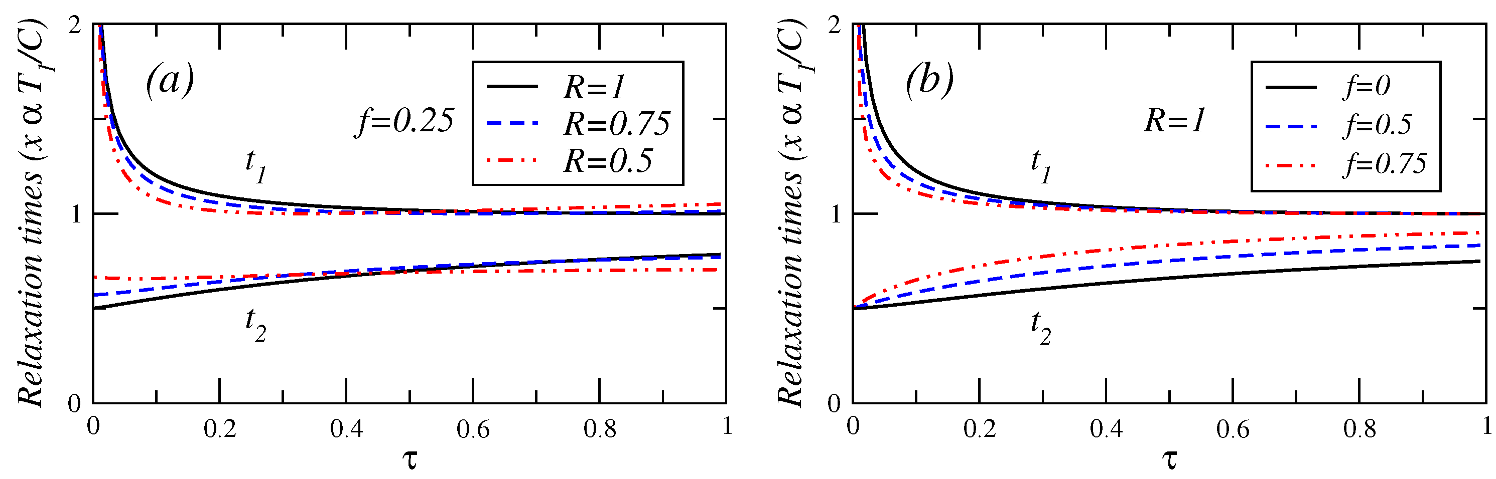
In Figure 4, Figure 5 and Figure 6, the relaxation times are plotted against τ for different values of fractional fuel cost f, for a fixed value of R ($R=1$), that is, the endoreversible case. It is observed that $t_1$ (Equation (A.8)) is a decreasing function of τ. This relaxation time decreases as the fuel cost increases, indicating a faster decay as $f⟶1$. For $t_2$ (see Equation (A.9)), this relaxation time remains almost constant for $f=0$. As the fractional fuel cost f increases, $t_2$ slowly increases too. In the limit $f⟶1$, both relaxation times tend to be closer each other, but there is a stronger inequality $t_2<t_1$ in the interval $0<\mathsf{\tau }<1$. These figures also show the relaxation times as a function of τ, for several values of the parameter R, and for a fixed value of the fractional fuel cost f. These figures show that $t_1$ is a decreasing function of τ and decreases as the parameter R decreases and $t_2$ remains almost constant when the irreversibility parameter changes. From the findings shown in Figure 4, Figure 5 and Figure 6, it is concluded that the system is stable for $\mathsf{\tau }>0$. As the fractional fuel cost f increases, $t_1$ decreases whereas $t_2$ increases, for a given value of R. In contrast, for a given value of f, as the irreversibility parameter R decreases, $t_1$ decreases, whereas $t_2$ increases (see phase portrait [3] where the phase diagram are showed in details). The power output and the efficiency depend on τ for the cases analyzed here, and both energetic quantities are decreasing functions of this parameter, that is, the system’s stability moves in the opposite direction to that of the steady-state as P, η and τ varies.

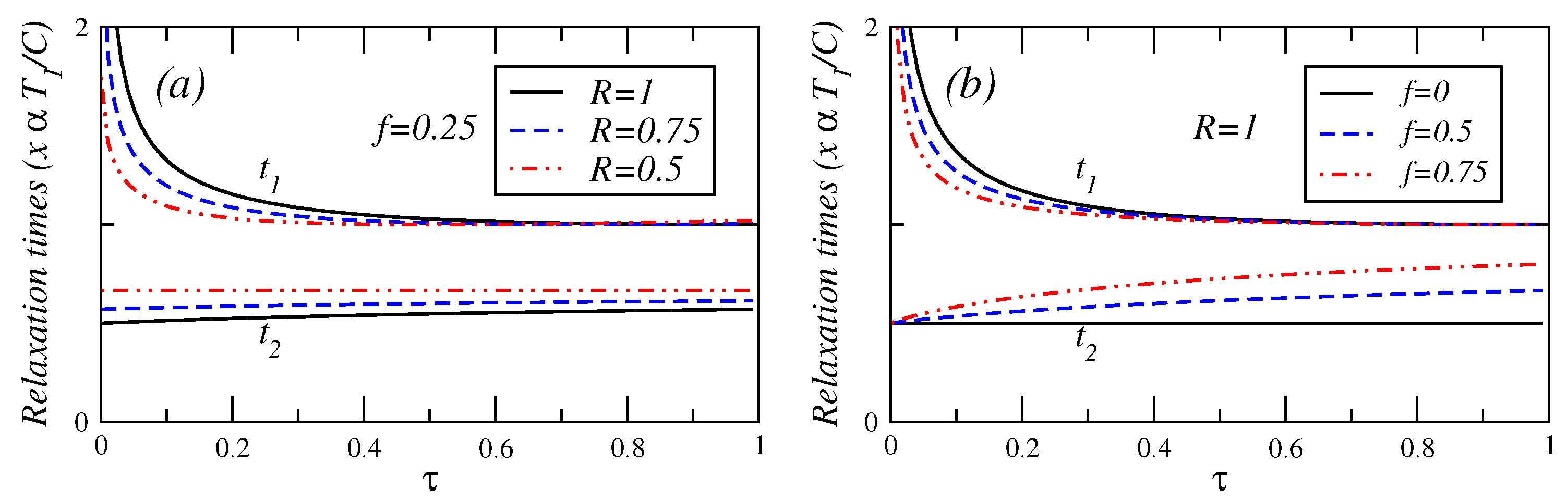
Figure 4. Plot of relaxation times under maximum power conditions versus τ for (a) several values of the endorreversibility parameter and a value of the fractional fuel cost and (b) for several values of the fractional fuel cost f in the endoreversible case (R = 1).

Figure 4. Plot of relaxation times under maximum power conditions versus τ for (a) several values of the endorreversibility parameter and a value of the fractional fuel cost and (b) for several values of the fractional fuel cost f in the endoreversible case (R = 1).

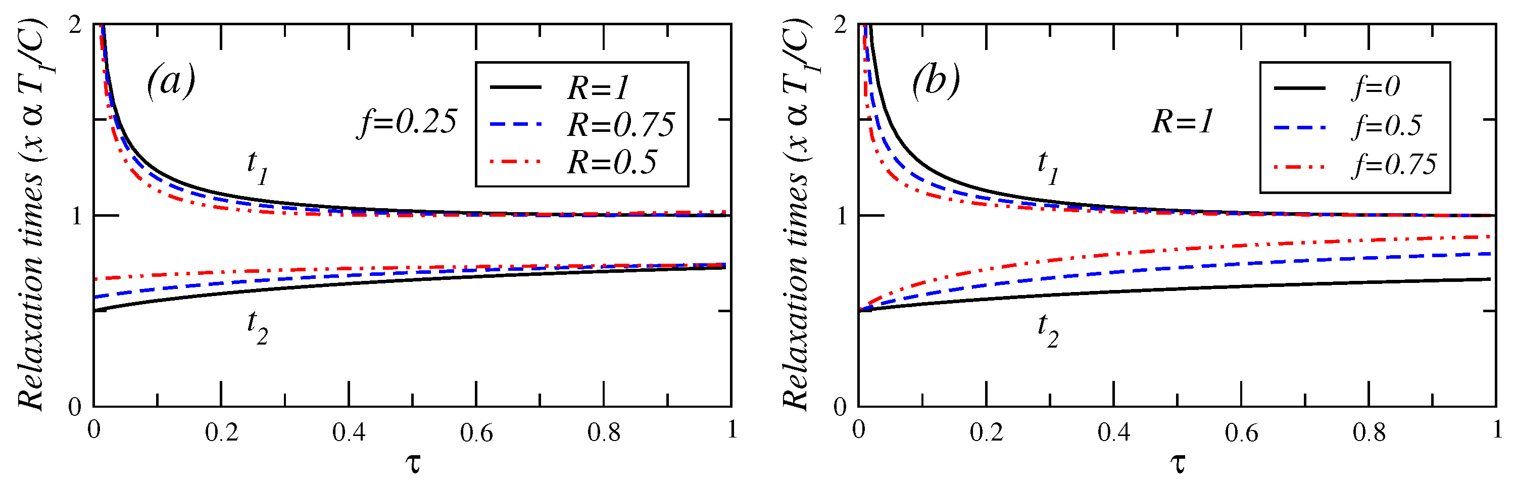
Figure 5. Plot of relaxation times under maximum efficient power versus τ for (a) several values of the endorreversibility parameter and a value of the fractional fuel cost and (b) for several values of the fractional fuel cost f in the endoreversible case (R = 1).

Figure 5. Plot of relaxation times under maximum efficient power versus τ for (a) several values of the endorreversibility parameter and a value of the fractional fuel cost and (b) for several values of the fractional fuel cost f in the endoreversible case (R = 1).

Figure 6. Plot of relaxation times under maximum ecological function conditions versus τ for (a) several values of the endorreversibility parameter and a value of the fractional fuel cost and (b) for several values of the fractional fuel cost f in the endoreversible case (R = 1).

Figure 6. Plot of relaxation times under maximum ecological function conditions versus τ for (a) several values of the endorreversibility parameter and a value of the fractional fuel cost and (b) for several values of the fractional fuel cost f in the endoreversible case (R = 1).

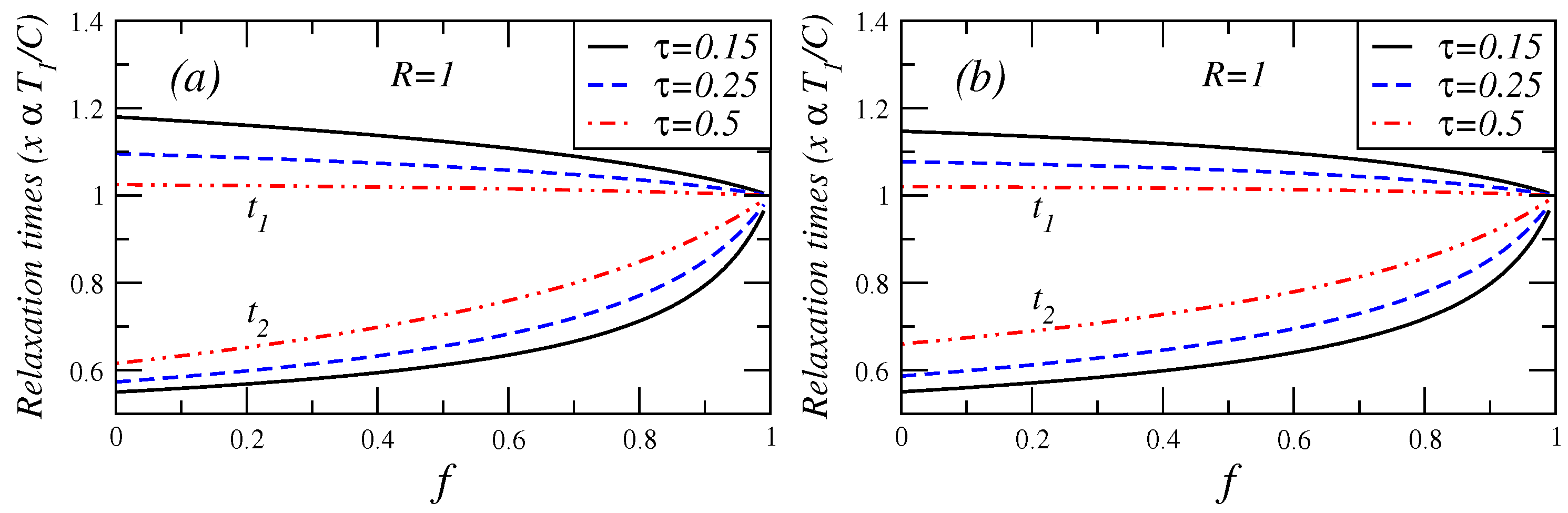
Additionally, in Figure 7, for the cases of maximum efficient power and maximum ecological function conditions, show the relaxation times versus fuel fractional cost for several values of τ. In these cases, it can be seen, how the fast (slow) relaxation time slightly increases (decreases) as f changes from 0 to 1.

Figure 7. Relaxation times in the endoreversible case ($R=1$) versus fractional fuel cost for several values of τ for (a) Maximum efficient power conditions and (b) Maximum ecological function.

Figure 7. Relaxation times in the endoreversible case ($R=1$) versus fractional fuel cost for several values of τ for (a) Maximum efficient power conditions and (b) Maximum ecological function.

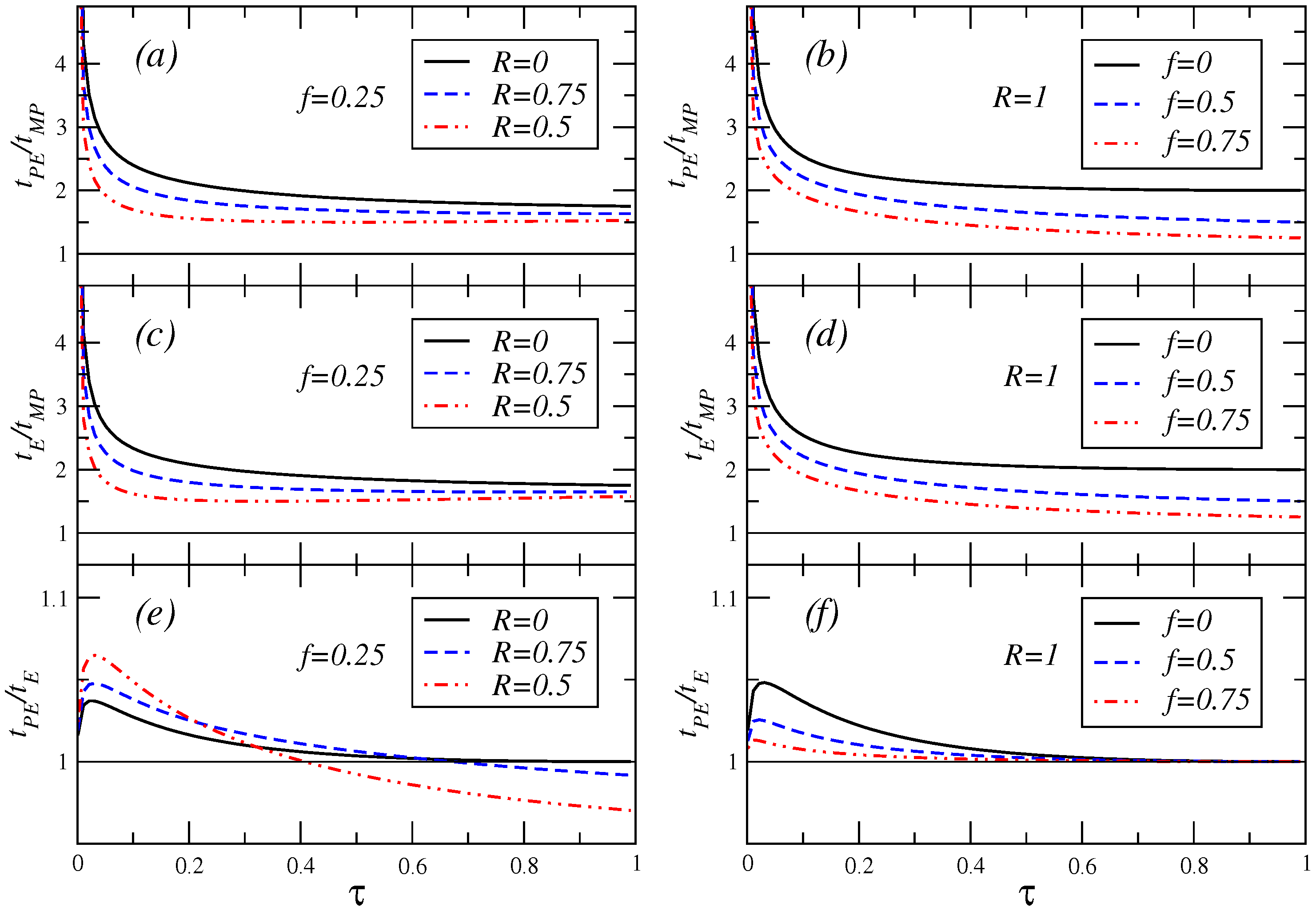
Finally, Figure 8 shows the ratio of the relaxation times previously calculated for the three regimes of operation considered. In this Figure, the inequality ${\mathsf{\tau }}_{EP}>{\mathsf{\tau }}_E>{\mathsf{\tau }}_{MP}$ holds.

Figure 8. Ratio of the relaxation times versus τ for a value of the fractional fuel cost and several values of the parameter R (cases (a), (c) and (e)), and for the endoreversible case $R=1$, for different values of the fractional fuel cost, (cases (b), (d) and (f)).

Figure 8. Ratio of the relaxation times versus τ for a value of the fractional fuel cost and several values of the parameter R (cases (a), (c) and (e)), and for the endoreversible case $R=1$, for different values of the fractional fuel cost, (cases (b), (d) and (f)).

4. Conclusions

This work presented a local stability analysis of a thermo-economic model of an irreversible heat engine working under different performance regimes: The Maximum Power Output, Maximum Efficient Power and the Ecological Function regime considering a linear heat transfer law (the Newtonian law case). The relaxation times are shown as function of α, C, τ, f and R; that is, they depend on the materials that separate the working fluid from the reservoirs (through α); and on the working fluid (through C); on the reservoir temperatures (through τ); on fractional fuel costs (through f, which is associated with several energy sources from renewable energy to natural gas, (see Table 1. reported by De Vos [5]) and on the internal irreversibilities (through R). After a small perturbation, the system exponentially declines to the steady state characterized by two different relaxation times. In addition, the relaxation time under maximum efficient power conditions is less than the relaxation times under both maximum ecological function and maximum efficient power; that is, under maximum efficient power conditions, there is better stability conditions than for the other two regimes, although these differences are not large. Our cycle model is an FTT simple version of a Carnot-type engine, but, additionally, it considers the fractional fuel costs. Finally, the results confirm the local stability properties of the CA-engine for the three performance regimes.