Sub-Quantum Thermodynamics as a Basis of Emergent Quantum Mechanics

Austrian Institute for Nonlinear Studies, Akademiehof, Friedrichstrasse 10, 1010 Vienna, Austria
Entropy 2010, 12(9), 1975-2044; https://doi.org/10.3390/e12091975
Submission received: 27 August 2010
/
Accepted: 2 September 2010
/
Published: 10 September 2010
(This article belongs to the Special Issue Nonequilibrium Thermodynamics)
Abstract
:This review presents results obtained from our group’s approach to model quantum mechanics with the aid of nonequilibrium thermodynamics. As has been shown, the exact Schrödinger equation can be derived by assuming that a particle of energy
is actually a dissipative system maintained in a nonequilibrium steady state by a constant throughput of energy (heat flow). Here, also other typical quantum mechanical features are discussed and shown to be completely understandable within our approach, i.e., on the basis of the assumed sub-quantum thermodynamics. In particular, Planck’s relation for the energy of a particle, the Heisenberg uncertainty relations, the quantum mechanical superposition principle and Born’s rule, or the “dispersion of the Gaussian wave packet”, a.o., are all explained on the basis of purely classical physics.
Keywords:
nonequilibrium thermodynamics; dissipative systems; diffusion wave fields; quantum mechanics; Schrödinger equation; uncertainty relations; superposition principle; Born’s rulePACS Codes:
03.65.-w; 03.65.Ta; 05.40.-a; 05.70.Ln1. Introduction
Considering a theory as emergent if it “contains or reduces to another theory in a significant manner or if its laws are tied to those of another theory via mathematical connections” [1], it is proposed that quantum mechanics is such a theory. More precisely, it is proposed that quantum theory emerges from a deeper, more exact theory on a sub-quantum level. In our approach, one assumes that the latter can be described with the aid of nonequilibrium thermodynamics. We ask ourselves how quantum theory would have evolved, had the “tool” of modern nonequilibrium thermodynamics existed, say, a century ago. As has recently been shown, one can derive the exact Schrödinger equation with said tool, where the relation between energy
and frequency
, respectively, is used as the only empirical input,
[2,3], with the additional option that even the appearance of Planck’s constant,
, may have its origin in classical physics [4]. For an extensive review of refs. [2] and [3], and for connections to similar work, and, in particular, to Fisher information techniques, see [1]. As to approaches in a similar spirit, see, for example, [5,6,7,8,9,10,11], and [12].
In the present review, we shall more generally summarize the results of our works relating to the derivation from purely classical physics of the following quantum mechanical features:
- Planck’s relation for the energy of a particle,
- the Schrödinger equation for conservative and non-conservative systems,
- the Heisenberg uncertainty relations,
- the quantum mechanical superposition principle,
- Born’s rule, and
- the quantum mechanical “decay of a Gaussian wave packet”.
Moreover, the energy spectrum of a quantum mechanical harmonical oscillator is derived classically, as well as that of a “particle in a box”, the latter thereby providing both a resolution of an objection by Einstein, and a clarification w.r.t. the differences between the de Broglie-Bohm interpretation and the present approach, respectively.
Further, it will be proven that free quantum motion exactly equals sub-quantum anomalous (i.e., “ballistic”) diffusion, and, via computer simulations with coupled map lattices, it will be shown how to calculate averaged (Bohmian) trajectories purely from a real-valued classical model. This is illustrated with the cases of the dispersion of a Gaussian wave packet, both for free quantum motion and for motion in a linear (e.g., gravitational) potential. The results are shown to be in excellent agreement with analytical expressions as they are obtained both via our approach, and also via the Bohmian theory. However, in the context of the explanation of Gaussian wave packet dispersion, quantitative statements on the trajectories’ characteristic behavior are presented, which cannot be formulated in any other existing model for quantum systems. Finally, an outlook is provided on some of the possible next steps of our thus presented research program.
As is well known, the main features of quantum mechanics, like the Schrödinger equation, for example, have only been postulated, but never derived from some basic principles. (Cf. Murray Gell-Mann: “Quantum mechanics is not a theory, but rather a framework within which we believe any correct theory must fit.” [13]) Even in causal interpretations of the quantum mechanical formalism, such as the de Broglie-Bohm theory, the quantum mechanical wave function, or the solution of the Schrödinger equation, respectively, is taken as input to the theory (sometimes even as a “real” ontological field), without further explanation of why this should have to be so. Still, the Bohmian approach has brought some essential insight into the nature of quantum systems, particularly by exploiting the physics of the “guiding equation” (in what is called “Bohmian mechanics”) or, respectively, by providing a detailed analysis of the “quantum potential”. The latter was shown, in the context of the Hamilton-Jacobi theory, to represent the only difference to the dynamics of classical systems. [14]
However, in 1965, Edward Nelson suggested a derivation of the Schrödinger equation from classical, Newtonian mechanics via the introduction of a new differential calculus. [15] Thus it was possible to show, e.g., that the quantum potential can be understood as resulting from an underlying stochastic mechanics, thereby referring to a hypothesized sub-quantum level. However, ambiguities within said calculus, e.g., as to the formula for the mean acceleration, as well as an apparent impossibility to cope with quantum mechanical nonlocality (which had become rather firmly established in the meantime) has led to a temporary decline of interest in stochastic mechanics. Still, it is legitimate to enquire also today whether the stochastic mechanics envisioned is not just one part of a necessarily larger picture, with the other part(s) of it yet to be established.
Considering the history of quantum mechanics, for example, with its many differences in emphasizing particle and wave aspects of quantum systems, one must concede that in general the particle framework was the dominant one throughout the twentieth century. (Cf., as a representative example, Richard Feynman: “It is very important to know that light behaves like particles, especially for those of you who have gone to school, where you were probably told about light behaving like waves. I’m telling you the way it does behave — like particles.” [16]) However, a purely particle-centered approach may not be enough, as the quantum phenomena to be explained may just be more complex than to be reducible to a one-level point-particle mechanics only. In other words, it is possible that by the attempts to reduce quantum dynamics to simple point-by-point interactions, the phenomenon to be discussed would remain without reach, because it is too complex to be described on just one (i.e., an assumed “basic”) level. In still other words, a quantum system may be an emergent phenomenon, where a stochastic point-mechanics on just one level of description would still be a necessary ingredient for its description, but not the only relevant one. So, there may exist two or more relevant levels (e.g., on different time and/or spatial scales), where only the combination, or interactions, of them would result in the possibility to completely describe quantum systems. The latter may thus be more complex than it is assumed in any one-level stochastic mechanics model. In fact, recent results from classical physics suggest that this more complex scenario is even highly probable, since the said new results exhibit phenomena which previously were considered to be possible exclusively as quantum phenomena.
One is here reminded of Feynman’s famous discussion of the double slit, and his introductory remark: “We choose to examine a phenomenon which is impossible, absolutely impossible, to explain in any classical way and has in it the heart of quantum mechanics. In reality, it contains the only mystery.” [17] However, the above-mentioned recent classical physics experiments not only disprove Feynman’s statement w.r.t. the double slit, but prove that a whole set of “quantum” features can be shown to occur in completely classical ones, among them being the Heisenberg uncertainty principle, indeterministic behaviour of a particle despite a deterministic evolution of its statistical ensemble over many runs, nonlocal interaction, tunnelling, and, of course, a combination of all these. I am referring to the beautiful series of experiments performed by the group of Yves Couder (see, for example, [18,19,20,21]) using small liquid drops that can be kept bouncing on the surface of a bath of the same fluid for an unlimited time when the substrate oscillates vertically. These “bouncers” can become coupled to the surface waves they generate and thus become “walkers” moving at constant velocity on the liquid surface. A “walker” is defined by a lock-in phenomenon so that the drop falls systematically on the forward front of the wave generated by its previous bouncings. It is thus a “symbiotic” dynamical phenomenon consisting of the moving droplet dressed with the Faraday wave packet it emits. In reference [19], Couder and Fort report on single-particle diffraction and interference of walkers. They show “how this wavelike behaviour of particle trajectories can result from the feedback of a remote sensing of the surrounding world by the waves they emit”. Of course, the “walkers” of Couder’s group, despite showing so many features they have in common with quantum systems, cannot be employed one-to-one as a model for the latter, with the most obvious difference being that quantum systems are not restricted to two-dimensional surfaces. However, along with the understanding of how the Schrödinger equation can be derived via nonequilibrium thermodynamics ([2,3]), also the mutual relationship of particle and wave behaviour has become clearer. Just as in the experiments with walkers, there exists an average orthogonality also for particle trajectories and wave fronts in the quantum case. This is going to be of central importance for our modelling of quantum mechanics with the aid of an assumed sub-quantum thermodynamics.
In the remainder of this introduction, a first sketch shall be given of how the said modelling can be carried out. At first, and foremost, we observe that the so-called “vacuum” unambiguously turned out during the twentieth century to be permeated by what is generally called the “zero-point energy”, or “zero-point fluctuations”, respectively, i.e., by a residual field in any accessible spacetime volume, even as the temperature
goes toward
. Also, any particle of nature has turned out to be characterized by a fundamental angular frequency
(i.e., in its rest frame) such that its total energy
is described by Planck’s relation,
, where
is the reduced Planck’s constant,
.
So, if there were only one particle in the world, the totality of such a universe would consist of an oscillator (i.e., our “particle” characterized by
) and its environment, i.e., the all-pervasive field of the zero-point fluctuations. Therefore, to start with, we shall investigate possible models for the dynamics between the said oscillator and the said vacuum fluctuations. From a thermodynamical viewpoint, then, it is clear that one will in general have to employ a nonequilibrium scenario. For, any oscillating system in nature is the result of a dissipative process, so that the mentioned frequency
can be understood as belonging to the properties of driven, off-equilibrium steady-state systems maintained by a permanent throughput of (kinetic) energy. Of course, for our single oscillator, the said energy must come from the zero-point energy, or, more precisely, the energy throughput for the maintenance of
is determined, respectively, by the absorption from and the dissipation into the zero-point energy field of the particle’s environment.
In this context, it is helpful to return again to the above-mentioned experiments of Couder’s group. To guide our imagination, the following analogy may be considered. As the “bouncer” in the said experiments both oscillates due to being driven by the surrounding waves and causes the emission of radially symmetrical waves into the environment, with a self-sustained phase-locking mechanism guaranteeing coherent oscillations of bouncer and surrounding medium, respectively, one may in a first approximation also consider the frequency
of a quantum as representing a similarly emergent “symbiotic” process. In other words, we consider a quantum “particle” as a dissipative phase-locked steady state, where an amount of zero-point energy of the wave-like environment is absorbed by the particle, and then, during a characteristic relaxation time
, dissipated into the environment again. In the simplest scenario of a universe with only one particle in it, this dissipation will occur radially-symmetrically, thus creating a (thermal) wave, or rather, maintaining the zero-point energy’s wave-like structure through the phase-locking.
In what follows it will be shown that if one considers such a corresponding free quantum particle along a single path, its description cannot be distinguished from that of a classical particle. That is, in this case the quantum potential will vanish identically. The said vanishing quantum potential is then proven to be exactly equivalent to a classical heat (diffusion) equation, the solutions of which are given as radially symmetric thermal diffusion wave fields. In other words, a non-vanishing quantum potential is thus generally an expression of a particle’s surrounding diffusion wave field scenario when that radial symmetry is broken by “something else” in the thus established more complex universe, i.e., in the cases when the particle is not free (or not facing a single, possible path, respectively). The gradient of the quantum potential will then be described as a completely “thermalized” fluctuating force field, where the origin of the latter is exactly identical to the zero-point fluctuation field.
So, our modelling approach will consist of two basic steps. In a first step, we just consider the simple “one particle in the universe” scenario, with the particle as the origin of thermal waves in synchrony with the surrounding medium. (Note that these thermal waves themselves could be considered as emerging from millions of millions of individual sub-quantum Brownian motions, but we are here interested only in the emergent waves and their possible interactions with others.)
In a second step, we consider the particle’s environment to be more realistic, i.e., the simple regular zero-point energy oscillations will then have to be substituted by oscillations within constraints, as, e.g., given by an experimental setup in which our particle is embedded. Then, even a single particle may not be considered as being free in general. For example, even the description of a source of quantum particles represents constraints on an otherwise unconstrained zero-point energy environment. Representing an initial particle distribution in some experimental setup by a Gaussian, for example, already implies that the heat of the zero-point field will be “squeezed” (i.e., within the limits of a “Gaussian slit”, for example). This squeezing, then, is equivalent to a non-vanishing fluctuating force on the particle. In other words, the first step in our modelling procedure basically refers to an oscillator and a radially symmetric diffusion wave field. The second step, however, will have to employ a stochastic element in order to account for the interactions of many different (though phase-locked) diffusion waves, thus referring directly to the zero-point fluctuations of the embedding environment and the effective Brownian-type “jumps” of our bouncer within the given geometric (and “vacuum compressing”) constraints of the setup.
In the following chapters, we shall employ this two-steps strategy twice. To begin with, we shall concentrate on the question of the appearance of
in a classical context, i.e., in a simple “driven harmonic oscillator” scenario, and then move to include a stochastic level, thus referring also to a fluctuating environment. Later, when concretely modelling the quantum mechanical dispersion of a Gaussian wave packet with classical means, we shall again start with the simple scenario of undisturbed diffusion waves, only to be modified in a second step to include the more realistic stochasticity of the processes involved. We shall then see that the model exactly reproduces the quantum mechanical results.
2. The “Walking Bouncer”: A Classical Explanation of Quantization
2.1. Introduction
In references [2,3], the Schrödinger equation was derived in the context of modelling quantum systems via nonequilibrium thermodynamics, i.e., by the requirement that the dissipation function, or the time-averaged work over the system of interest, vanish identically. The “system of interest'” is a “particle” in terms of a harmonic oscillator embedded in a thermal environment of non-zero average temperature (i.e., of the “vacuum”). In more recent papers, we have illustrated the “particle” more concretely by using the concept of a “bouncer” (or “walker”, respectively) gleaned from the beautiful experiments by Couder's group [18,19,20,21]. Thus we assume that the thermal environment is oscillating itself, with the kinetic energy of these latter oscillations providing the energy necessary for the “particle” to maintain a constant energy, i.e., to remain in a nonequilibrium steady state. Regarding the respective (“zero-point”) oscillations of the vacuum, we simply assume the particle oscillator to be embedded in an environment comprising a corresponding energy bath. [4]
2.2. A Classical Oscillator Driven by Its Environment’s Energy Bath: The “Bouncer”
Let us start with the following Newtonian equation for a classical oscillator
Equation (2.2.1) describes a forced oscillation of a mass
swinging around a center point along
with amplitude
and damping factor, or friction,
. If
could swing freely, its resonant angular frequency would be
. Due to the damping of the swinging particle there is a need for a locally independent driving force
.
We are only interested in the stationary solution of Equation (2.2.1), i.e., for
, where
plays the role of a relaxation time, using the ansatz
After a short calculation we find for the phase shift between the forced oscillation and the forcing oscillation that
and for the amplitude of the forced oscillation
To analyse the energetic balance, we multiply Equation (2.2.1) with
and obtain
and thus,
where the first term within the brackets is the kinetic energy and the second one is the potential energy of the oscillator system. Therefore, the time-derivative of the sum must be zero since the sum is the whole energy of the system and has hence to be of constant value.
Due to the friction the oscillator looses energy to the energy bath, represented by
, whereas
represents the energy which has to be regained from the energy bath via the force
. The two terms on the right-hand side must also be zero and we can hence write down the net work-energy that is taken up from the bouncer in the form of heat during each period
as
Inserting
from Equation (2.2.4), we can see that
at
, in which case the energy reaches its maximum.
To derive the stationary frequency
, we use the right-hand side of Equation (2.2.6) together with Equation (2.2.2) and obtain
As all factors, except for the sinusoidal ones, are time independent, we have the necessary condition for the phase given by
for all
. Substituting this into Equation (2.2.3), we obtain
and thus
Therefore, the system is stationary at the resonance frequency of the free undamped oscillator. With the notations
we obtain
The Hamiltonian of the system is the term within the brackets on the left-hand hand side of Equation (2.2.6),
We introduce the angle
and substitute Equation (2.2.2) into Equation (2.2.14), thus yielding the two equations
and
From Equation (2.2.16), an invariant quantity is obtained: it is the angular momentum
With
, the quantity of Equation (2.2.17) becomes the time-invariant expression of a basic angular momentum, which we denote as
Thus, we rewrite our result (2.2.13) as
2.3. Brownian Motion of a Particle: The “Walker”
Now we concentrate on the motion of our “bouncer” within a more irregular environment. That is, we now assume that the “particle” is not only driven via harmonic oscillation of a wave-like environment, but that there is also a stochastic element in its movement, as, e.g., due to different fluctuating wave-like configurations in the environment. Therefore, our “particle’s” motion will assume a Brownian-type character. The Brownian motion of a thus characterized particle (which we propose to call a “walker”), is then described by a Langevin's stochastic differential equation with velocity
and a force
,
with a friction coefficent
. The time-dependent force
is stochastic, i.e., one has as usual for the time-averages
where
differs noticeably from zero only for
. The correlation time
denotes the time during which the fluctuations of the stochastic force remain correlated.
The standard textbook solution of Equation (2.3.1) in terms of the mean square displacements
is given (e.g., in [22]) by the Ornstein-Uhlenbeck equation, with
now being the “vacuum” temperature,
Note that, on the one hand, for
, and by expanding the exponential up to second order, Equation (2.3.3) provides that
On the other hand, for
one obtains the familiar relation for Brownian motion, i.e.,
with the “diffusion constant” D given by
Now we remind ourselves that we have to do with a steady-state system. Just as with the friction
there exists a flow of (kinetic) energy into the environment, there must therefore also exist a work-energy flow back into our system of interest. For its calculation, we multiply Equation (2.3.1) by
and obtain an energy-balance equation. It yields for the duration of time
, with the natural number
chosen so that
is large enough to make all fluctuating contributions negligible, the net work-energy of the walker
We require that our particle attain thermal equilibrium ([2,3]) after long times so that, for each degree of freedom, the average value of the kinetic energy becomes, as usual,
We thus obtain
where
equals the period of Equation (2.2.7), which is chosen in order to make the result comparable with Equation (2.2.19). The work-energy for the particle undergoing Brownian motion can thus be written as
2.4. The “Walking Bouncer”: Derivation of
Let us summarize what we have achieved so far. We have for both systems, i.e., oscillator and particle in Brownian-type motion (or “bouncer” and “walker”, respectively), obtained a net work-energy flow into each system, respectively, in order to compensate for the respective energy losses due to friction. There is a continuous flow from the bath to the oscillator, and vice versa. Moreover, and most importantly, during that flow, for long enough times
, the friction of the bouncer can be assumed to be exactly identical with the friction of the walker. For this reason we directly compare the results of Equations (2.2.19) and (2.3.10),
Providing
Now, one generally has that the total energy of a sinusoidal oscillator exactly equals twice its average kinetic energy. Moreover, despite having a nonequilibrium framework of our system, the fact that we deal with a steady state means that our oscillator is in local thermal equilibrium with its environment. As the average kinetic energy of the latter is always given by
, one has for the total energy that
. Now, one can express that energy via (2.4.2) in terms of the oscillator’s frequency
, and one obtains
Assuming the same friction coefficient for both the bouncer and the walker,
, we obtain the energy balance between oscillator and its thermal environment as
with the total energy of our model for a quantum “particle”, i.e., a driven steady-state oscillator system, being now derived as
Moreover, if we compare Equation (2.4.4) with the Langevin equation (2.3.1), we find the following confirmation of Equation (2.4.5). First, we recall Boltzmann’s relation between the heat applied to an oscillating system and a change in the action function
, respectively, [2,3] providing
relates to the momentum fluctuation via
where, as usual [2,3],
Thus one obtains with (2.4.4) that the friction in (2.3.1) is given by
Then, as
, with Equation (2.4.4) for the thermal bath as above, and with Equation (2.4.6) one obtains
and the friction term
Note that with Equations (2.4.4) and (2.4.10), one obtains the expression for the diffusion constant
which is exactly the usual expression for
in the context of quantum mechanics.
With (2.4.11) one can also introduce the recently proposed concept of an “entropic force” [23]. That is, with the total energy equaling a total work applied to the system, one can write (with
denoting the entropy)
Equation (2.4.13) provides an “entropic” view of a harmonic oscillator in its thermal bath. First, the total energy of a simple harmonic oscillator is given as
. Now, the average kinetic energy of a harmonic oscillator is given by half of its total energy, i.e., by
, which --- because of the local equilibrium --- is both the average kinetic energy of the bath and that of the “bouncer” particle. As the latter during one oscillation varies between
and
, one has the following entropic scenario. When it is minimal, the tendency towards maximal entropy will provide an entropic force equivalent to the absorption of the heat quantity
. Similarly, when it is maximal, the same tendency will now enforce that the heat
is given off again to the “thermostat'” of the thermal bath. In sum, then, the total energy throughput
along a full circle will equal, according to (2.4.13),
. In other words, the formula
does not refer to a classical “object” oscillating with frequency
, but rather to a process of a “fleeting constancy”: due to entropic requirements, the energy exchange between bouncer and heat bath will constantly consist of absorbing and emitting heat quantities such that in sum the “total particle energy” emerges as
[4].
2.5. Energy Spectum of the Harmonic Oscillator from Classical Physics
A characteristic and natural feature of nonequilibrium steady state systems is given by the requirement that the time integral of the so-called dissipation function
(to be discussed in more detail in the next chapter) over full periods
vanishes identically [2]. Assuming that our oscillator has a characteristic frequency
, one defines the dissipation function w.r.t. the force in Equation (2.2.1) over the integral
Here, we assume a generalized driving force
to have a periodic component such that
. Then one generally has that
and so the requirement (2.5.1) generally provides that
(Incidentally, this condition resolves the problem discussed by Wallstrom [24] about the single-valuedness of the quantum mechanical wave functions and eliminates possible contradictions arising from Nelson-type approaches to model quantum mechanics on a “particle centered” basis alone.)
So, we are dealing with a situation where a “particle” oscillates with an angular frequency
driven by the external force due to the surrounding (“zero-point”) fluctuation field, with a period
. For the type of basic oscillation we have assumed a simple harmonic motion, or, equivalently [17], circular motion, and we generally have that the total (“zero-point”) energy is
(In fact, (2.5.4) also turns out to equal the average quantum potential
. [3]) Then, for slow, adiabatic changes during one period of oscillation, the action function over a cycle is an invariant,
with
. This provides, in accordance with the corresponding standard relation for integrable conservative systems [2], i.e.,
that
However, the external driving frequency and the particle’s basic frequency
, respectively, are not just in simple synchrony, since one has to take into account also the type of energy exchanges of the “particle” with its oscillating environment as discussed in the previous section. Generally, there exists the possibility (within the same boundary condition, i.e., on the circle) of periods
, with
, of adiabatical heat exchanges “disturbing” the simple particle oscillation as given by Equation (2.5.4). That is, while we have so far considered, via Equations (2.5.5) and (2.5.6), a single, slow adiabatic change during an oscillation period
, we now also admit the possibility of several (i.e.,
) periodic heat exchanges during the same period, i.e., absorptions and emissions as in (2.4.13). The action integrals over full periods then more generally become
Thus, one can first recall the expressions (2.5.4) and (2.5.7), respectively, to obtain for the case of “no additional periods” () the basic “zero-point” scenario
Secondly, however, using (2.5.3), one obtains for n =1, 2,... that
This provides a spectrum of
additional possible energy values,
such that, together with Equation (2.5.9), the total energy spectrum of the off-equilibrium steady-state harmonic oscillator becomes
Note that to derive Equation (2.5.12) no Schrödinger or other quantum mechanical equation has been used. Rather, it was sufficient to invoke Equation (2.5.2), without even specifying the exact expression for
.
In this chapter we derived Planck’s relation
from classical physics. This was made possible by the identification of
with the angular momentum (2.2.18),
, of our basic oscillator. What yet remains to be shown is the universality of this relation, i.e., that it holds for any particle with any mass
. Note, however, that there exists a possibly related explanation of the universality of
based on a thermodynamic analysis of the harmonic oscillator, i.e., T. Boyer’s derivation [25], given in the context of a classical physics in the presence of a (“classical”) zero-point energy field.
3. Derivation of the Exact Schrödinger Equation from Classical Physics
3.1. Introduction
Based on the results of the foregoing chapter, it already follows from classical physics, that to each particle of nature one associates an energy
As it is well known that oscillations in general are the result of dissipative processes, the frequencies
can be understood within the framework of nonequilibrium thermodynamics, or, more precisely, as properties of off-equilibrium steady-state systems maintained by a permanent throughput of energy from the environment.
So, we deal here with a “hidden” thermodynamics, out of which the known features of quantum theory should emerge. (This says, among other things, that we do not occupy ourselves here with the usual quantum versions of thermodynamics, out of which classical thermodynamics is assumed to emerge, since we intend to deal with a level “below” that of quantum theory, to begin with.)
Of course, there is a priori no guarantee that nonequilibrium thermodynamics is in fact operative on the level of a hypothetical sub-quantum “medium”, but, as will be shown here, the straightforwardness and simplicity of how the exact central features of quantum theory emerge from this ansatz will speak for themselves. Moreover, one can even reverse the doubter’s questions and ask for compelling reasons, once one does assume the existence of some sub-quantum domain with real physics going on in it, why this medium should not obey the known laws of, say, statistical mechanics. For, one also has to bear in mind, a number of physical systems exhibit very similar, if not identical, behaviours at vastly different length scales. For example, the laws of hydrodynamics are successfully applied even to the largest structures in the known universe, as well as on scales of kilometres, or centimetres, or even in the collective behaviour of quantum systems. In short, although there is no a priori guarantee of success, there is also no principle that could prevent us from applying present-day thermodynamics to the sub-quantum regime.
What is proposed here can also be considered as a gedanken experiment: what if our knowledge of classical physics (including wave mechanics and nonequilibrium thermodynamics) of today had been available 100 years ago? The answer is as follows: One could have thus, without any further assumptions or any ad hoc choices of constants, derived the exact Schrödinger equation, both for conservative and non-conservative systems, using only universal properties of oscillators and nonequilibrium thermostatting. It is particularly the latter feature which is rather appealing, since the use of universality properties guarantees model independence. That is, it will turn out unnecessary to have much knowledge about the detailed sub-quantum mechanisms, as the universal properties of the systems in question will be shown to suffice to obtain the results looked for. Moreover, the approach to be presented here not only re-produces the Schrödinger equation, but also puts forward some new results, such as the sub-quantum fluctuation theorem, which can thus help shed light on problems not properly understood today within the known quantum formalism.
In section 2 of this chapter, a short review is given of some results from nonequilibrium thermodynamics, which are particularly useful for our purposes. Section 3 then presents the application of the corresponding sub-quantum modelling of conservative systems, thus providing a straightforward derivation of the Schrödinger equation from modern classical physics. It is claimed that this represents the only exact derivation of the Schrödinger equation from classical physics in the literature. In section 4, then, the scheme is extended to include the Schrödinger equation for integrable non-conservative systems. Finally, the more encompassing scope of the present approach is presented, culminating in a formulation and discussion of the “vacuum fluctuation theorem”, with particular emphasis being put on possible applications for a better understanding of quantum mechanical nonlocality.
3.2. Some Results from Nonequilibrium Thermodynamics
In the thermodynamics of small objects, the interactions with their environments are dominated by thermal fluctuations. Since the 1980ies, new experimental and theoretical tools have been developed to provide a firm basis for a theory of the nonequilibrium thermodynamics of small systems. Most characteristic for such systems are the irreversible heat losses between the system and its environment, the latter typically being a thermal bath. In recent years, a unified treatment of arbitrarily large fluctuations in small systems has been achieved by the formulation of so-called fluctuation theorems (FT). One type of FT has been developed by G. Gallavotti and E. Cohen [26] and deals with steady-state systems.
Steady-state systems are characterized by an external agent continuously producing heat which thus contributes to the small system’s heat bath. The rate at which the system exchanges heat with this bath is given by the entropy production
, where the entropy
, with
being the temperature and
the time interval over which the system exchanges the heat
. Gallavotti and Cohen associate the entropy production with a time-dependent probability distribution in phase space,
, and their FT provides an expression for the ratio of the probability of absorbing a given amount of heat versus that of releasing it:
where
is Boltzmann’s constant.
Practically, Equation (3.2.1) also holds to good approximation for finite times, i.e., as long as
is much greater than a given decorrelation time. Equation (3.2.1) expresses the fact that nonequilibrium steady-state systems on average always tend to dissipate heat rather than absorb it. Nevertheless, it also gives an exact probability for heat absorption (negative
), which still is non-zero. Generally, FTs give a new answer to an old question already discussed by Boltzmann and Loschmidt, among others: how does time-reversible Newtonian mechanics in the microscopic realm lead to the time-irreversible macroscopic equations of thermodynamics and hydrodynamics? FTs provide the answer by giving exact formulas for the ratio between the probability of a process in the forward-time direction and the corresponding probability in the reversed-time direction (cf. Equation (3.2.1)). If this ratio is equal to one, of course, one deals with the time-symmetric situation of classical mechanics. However, the new quality of FTs is given by the possibility to describe the transition from the time-reversible equations to those of irreversible macroscopic behaviour. It has turned out that microscopic violations of the Second Law for a finite time are possible (and have indeed been observed), but that the allowed fluctuations in the microscopic domain tend to become insignificant as soon as the system becomes macroscopic, because the above-mentioned ratio of probabilities grows exponentially with the system’s size, or with the length of observation time, respectively. Thus, for large systems, the conventional Second Law emerges. (For an excellent review, see Evans and Searles [27].)
Related to Equation (3.2.1), but actually more apt for our purposes, is a FT given by Williams, Searles, and Evans in 2004. [28] They consider what happens to a nonequilibrium dissipative system, where the initial conditions are assumed to be known, and where the system is maintained at a constant temperature. (We recall that, as an application, we want to treat the particles of quantum mechanics as such “small systems”, and it is natural to start with the suggestion that they are held at some constant temperature, at least in the free-particle case.)
If this small system is surrounded by a heat bath, and if the heat capacity of this thermal reservoir is much greater than that of the system, one can “expect the system to relax to a nonequilibrium quasi-steady-state in which the rate of temperature rise for the … system is so small that it can be regarded as being zero.” [28] In their paper, Williams et al. give a detailed analysis to show how their “transient” fluctuation theorem (TFT) is independent of the precise mathematical details of the thermostatting mechanism for an infinite class of fictitious time reversible deterministic thermostats. They thus prove the factual independence of their TFT from the thermostatting details, a fact which we denote as “universality of thermostatting” for nonequilibrium steady-state systems.
The kinetic temperature of the heat reservoir is defined by
where
is the Cartesian dimension of the system,
the number of reservoir particles,
their momenta and
their individual masses. Since the reservoir is very large compared to the small dissipative system, one can safely assume that the momentum distribution in this region is given by the usual Maxwell-Boltzmann distribution. This corresponds to a “thermostatic” regulation of the reservoir’s temperature. Now, if the phase space distribution function of trajectories
, i.e.,
, for the thermostatted system is known, Williams et al. show how the TFT can be applied. Instead of using the entropy production
as in Equation (3.2.1), the TFT now has to be formulated with the aid of a more generalized version of it, the so-called dissipation function
. It is defined by the following equation [28]:
where
is the initial
distribution of the particle trajectories
,
is the corresponding state at time
,
the initial distribution of those time evolved states, and
the phase space compression factor. Similar to Equation (3.2.1), the TFT now provides the probability ratio
The notation
is used to denote the probability that the value of
lies in the range from
to
, and
refers to the range from
to
.
Because of the equilibrium distribution of the thermostat, or, equivalently, because the energy lost to the thermostat can be regarded as heat, the phase space compression factor is essentially given by the heat transfer
,
and the first expression on the r.h.s. of Equation (3.2.3) is equal to the change of the total energy
, i.e.,
The authors are able to show that generally, when the number of degrees of freedom in the reservoir is much larger than the number of degrees of freedom in the small system of interest, the dissipation function is equal to the work
applied to the system,
By definition, the latter is given by [28]
where the dissipative field
does work on the system by driving it away from equilibrium,
is the so-called dissipative flux, and
the volume of interest. This work is converted into heat, which is in turn removed by the thermostatted reservoir particles, thus maintaining a nonequilibrium steady state.
Finally, substituting Equation (3.2.8) into Equation (3.2.4) provides the TFT implied by universal thermostatting (with the bars denoting averaging) [27]:
3.3. Merging Thermodynamics with Wave Mechanics: Emergence of Quantum Behaviour
3.3.1. The Basic Assumptions
From the beginning, early in the twentieth century, and onwards, quantum phenomena have been characterized by both particle and wave aspects. Let us take Equation (3.1.1),
, as the starting point for our approach, and note as an aside that the oscillations indicated by the frequency
can be considered as those of a carrier wave, which, depending on an observer’s rest frame, are modulated such that the free particle’s velocity is given by the group velocity of the associated wave. (The “free particle” is an idealization, with the particle considered to be un-affected by the thermodynamic “disturbances”, which will be introduced below. Still, in many cases, the average particle velocity will equal the group velocity even after those disturbances are accounted for.) From classical wave mechanics we then know that
, but we generally also have that
(i.e., with wave number
and momentum
), so that by comparison we thus obtain with Equation (3.1.1) that the particle’s momentum is given by de Broglie’s relation
So, one can imagine a particle as an oscillating entity which is in contact with its surroundings via a wave-like dynamics related to its frequency
. As we want to consider a classical wave, we can note that the probability density
for the presence of such a particle (which thus is equal to the detection probability density) is such that it coincides with the wave’s intensity
, with
being the wave’s (real-valued) amplitude (Assumption 1):
Now let us propose a central argument of our approach. We assume that a sub-quantum (nonequilibrium) thermodynamics provides the correct statistical mechanics responsible for the understanding of the oscillatory behaviour of a single particle on the quantum level. The “language” used is of course one of ensembles of (sub-quantum) particles, and the task is to find the appropriate transition to the ensemble behaviour of many particles (e.g., one particle in many consecutive runs of an experiment) on the quantum level. We propose that by merging the sub-quantum thermodynamics with classical wave mechanics, the emergence of quantum behaviour can be exactly modelled.
To do so, we must ask how the probability densities of a particle on the quantum level are constructed from the sub-quantum distribution functions (i.e., of
particle statistical mechanics). We propose that the temporal evolution of the quantum particle’s probability density in configuration space is an emerging property of the system’s description based on the underlying temporal evolution of the corresponding sub-quantum distribution function, i.e.,
The equilibrium distribution
according to Equation (3.2.6) is therefore assumed to be reflected also in the distribution
. In other words, the second “input” to our theory, is provided by the following proposition of emergence (Assumption 2): the relation between the distribution functions referring to the trajectories at the times
and
, respectively, on the sub-quantum level is mirrored by the corresponding relation between the probability densities on the quantum level:
In Equation (3.3.2) it is proposed that the many microscopic degrees of freedom associated with the sub-quantum medium are recast into the more “macroscopic” properties that characterize a collective wave-like behaviour on the quantum level. (This will imply that the buffeting effects of the surroundings on the particle are represented by a fluctuating force, as we shall see below.) Similar to the thermodynamics of a colloidal particle in an optical trap [29], the relevant description of the system is no longer given by the totality of all coordinates and momenta of the microscopic entities, but is reduced to only the particle coordinates.
This “emergence” of the ratio (3.3.2) on the quantum level can be justified on dynamical grounds. Assuming that the probability density (3.3.1) obeys the usual continuity equation, i.e.,
with solutions
we see that the exponent in Equation (3.3.4) exactly matches a familiar form of the phase space compression factor, i.e.,
As in this chapter we assume, to begin with, the strictly time-reversible case, the corresponding dissipation function (3.2.3) must vanish identically. Thus, if one allows for
to be defined by the restriction to
, then upon the combination of Eqations (3.3.4) and (3.3.5), Equation (3.3.2) follows immediately.
Finally, the proposal that the frequency
is maintained in a steady-state via the constant throughput of thermal energy has to be cast into a re-formulation of what is understood as “total energy”, i.e., of Equation (3.1.1). For the time being, we do not need to specify what exactly this thermal energy is, although we shall later identify it with the vacuum’s zero-point energy. All we need to specify in the beginning is that a quantum system’s energy consists of the “total energy” of the “system of interest” (i.e., the particle with frequency
), and of some term representing energy throughput related to the surrounding vacuum, i.e., effectively some function
of the heat flow
:
The first term is assumed to be given by Equation (3.1.1), and the second term, being equivalent to some kinetic energy, can be recast with the aid of a fluctuating momentum term,
, of the particle with momentum
. Thus, the total energy is given by (Assumption 3):
That is all we need: Equations (3.3.1), (3.3.2), and (3.3.7) suffice to derive the exact Schrödinger equation from (modern) classical physics. This shall be shown now.
3.3.2. Derivation of the Exact Schrödinger Equation from Classical Physics
We consider the standard Hamilton-Jacobi formulation of classical mechanics, with a “total internal energy” of the system of interest generally given by
where
is some potential energy. In the following, we shall for simplicity restrict ourselves to the one-particle case
, as an extension to the many-particle case can easily be done.
We introduce the action function
such that the total energy of the whole system (i.e., our “system of interest” and the additional kinetic energy due to the assumed heat flow) is given by
To start with, we consider as usual the momentum
of the particle as given by
noting, however, that this will not be the effective particle momentum yet, due to the additional momentum coming from the heat flow. With these preliminary definitions, we formulate the action integral in an
dimensional configuration space with the Lagrangian
as
where we have introduced the momentum fluctuation of Equation (3.3.7) as
Our task is now to derive an adequate expression for
from our central assumption, i.e., from an underlying nonequilibrium thermodynamics. To begin, we remember the distinction between “heat” as disordered internal energy on one hand, and mechanical work on the other: heat as disordered energy cannot be transformed into useful work by any means. According to Boltzmann, if a particle trajectory is changed by some supply of heat
to the system, this heat will be spent either for the increase of disordered internal energy, or as ordered work furnished by the system against some constraint mechanism [30]:
With
being the effect of a heat flow, Equation (3.3.13) is a corollary of Equation (3.2.7), where the work applied to the system effectively produces a heat flow. This is why
has different signs in the two respective equations. However, we first want to concentrate on time-reversible scenarios where
.
It is clear that for the limiting case of Hamiltonian flow, which is characterized by a vanishing phase space contraction (3.3.5), a time-reversible scenario is evoked where
for all times. However, one can also maintain time reversibility by choosing that only the time average vanishes,
, thus allowing for the system of interest to be a nonequilibrium steady-state one. So, in what follows we shall at first restrict ourselves to the case where on average no work is done,
, which is equal to the time-reversible scenario. In the consecutive Chapter, then, we shall consider the time-irreversible case,
.
If in Equation (3.2.7), or Equation (3.2.8), respectively, we therefore set
(which due to the specific form of these Equations per se already implies time averaging), the dissipation function
vanishes identically, which in turn confirms time reversibility. However, as
, we obtain with Eqations (3.2.3), (3.2.5), and (3.3.2) the probability (density) ratio
This is equivalent to the form of the usual Maxwell-Boltzmann distribution for thermodynamical equilibrium, but this time it is the result of universal thermostatting in nonequilibrium thermodynamics under the restriction that on average the work vanishes identically.
Now, in order to proceed in our quest to obtain an expression for the momentum fluctuation (3.3.12) from our thermodynamical approach, we can again rely on a formula originally derived by Ludwig Boltzmann. As mentioned above, Boltzmann considered the change of a trajectory by the application of heat
to the system. Considering a very slow transformation, i.e., as opposed to a sudden jump, Boltzmann derived a formula which is easily applied to the special case where the motion of the system of interest is oscillating with some period
. Boltzmann’s formula, which we already used in the previous chapter, relates the applied heat
to a change in the action function
, i.e.,
, providing [30,31]
This is in perfect agreement with the standard relation for integrable conservative systems, which we do deal with as long as we restrict ourselves to considering properties of our “system of interest”, providing an invariant action function
. As originally proposed by Ehrenfest and reformulated in Goldstein [32],
Identifying
with the heat flow
, and with
as just mentioned, Equation (3.3.16) provides exactly the relation (3.3.15) again. (We shall return to Equation (3.3.16) in Chapter 4, when we discuss the extension of our approach to non-conservative systems.)
Note that in Equation (3.3.15) we already have obtained a connection between the heat flow
and our looked-for momentum fluctuation
, the latter being given by Equation (3.3.12),
What remains to be identified with familiar expressions, is the term
in Equation (3.3.14). It refers to the apparent temperature of the surroundings of our system of interest, with the latter having a total internal energy
.
Now, just as Equation (3.3.14) was derived from very general, i.e., model-independent, features of nonequilibrium thermodynamics (“universal thermostatting”), we can now also give an alternative expression for the temperature of the thermostat from a very general observation. The latter is concerned with an already mentioned universal property of harmonic oscillators: All sinusoidal oscillations have the simple property that the average kinetic energy is equal to half of the total energy[17]. Now, our system of interest has the total internal energy of
, and we deal with steady-state systems where the internal temperature on average matches the external one of the surrounding medium. We thus obtain with the requirement that the average kinetic energy of the thermostat, Equation (3.2.2), must equal the average kinetic energy of the oscillator, that for each degree of freedom
(In fact, we have already derived the equality (3.3.17) in the previous chapter, viz., Equation (2.4.4).) Combining, therefore, Equations (3.3.14), (3.3.15), and (3.3.17), we obtain
Thus we obtain from Equation (3.3.18) our final expression for the momentum fluctuation
, derived exclusively from model-independent universal features of harmonic oscillators and nonequilibrium thermodynamical systems:
This further provides the expression for the additional kinetic energy term in Equation (3.3.11), i.e.,
As will be shown shortly, inserting Equation (3.3.20) into the action integral (3.3.11) will ultimately provide the Schrödinger equation. (For an earlier version, see [33], where also Heisenberg’s uncertainty principle is derived from Equation (3.3.19)).
Before doing so, the following remark may be helpful. There is an alternative way to derive the final action integral by referring in Equation (3.3.11) to a generalized average momentum
instead of the two kinetic energy terms. Then, instead of Equation (3.3.11) , there would only remain one term for the kinetic energy, given by
. However, as the average momentum fluctuations
must be linearly uncorrelated with the average momentum
, such that the (averaged) vector product is unbiased [34], one has the average orthogonality condition
such that the terms with mixed momentum components vanish identically and the action integral again is given by Equation (3.3.11). In fact, the requirement (3.3.21) is immediately obtained also from our requirement that the dissipation function, or the average work, respectively, vanishes identically. For, if we identify in Equation (3.2.8) the flux
as the probability density current, i.e.,
and if we characterize the external force
by the change in momentum
, i.e.,
the average work, assuming ergodicity, is given by
which thus confirms Equation (3.3.21), and, ultimately, the action integral (3.3.11). (We also note here that a posteriori, with the quantum physical equations already at our disposal, one can provide an additional, compulsory argument that necessarily confirms Equation (3.3.24), as will be shown later.) This concludes the remark.
Returning to our main line of reasoning, we now turn to the derivation of the Schrödinger equation. We begin by recalling the identity (3.3.1), i.e., of the probability density with the intensity of waves of amplitude
. (Note: This holds for the time-reversible scenario, which we deal with here. In general, this identity does not necessarily hold for nonequilibrium situations. [35]) Thus, the action integral we have arrived at now reads
where
Now we introduce the “Madelung transformation” (with the star denoting complex conjugation),
Thus one has
and one obtains a transformation rule between the formulations of modern classical physics and orthodox quantum theory: the square of the average total momentum is given by
With
from equation (3.3.27) one can rewrite (3.3.25) as
Further, with the identity
, one finally obtains the well-known Lagrange density
As given by the standard procedures of classical physics, this Lagrangian density provides (via the Euler-Lagrange equations) the Schrödinger equation
Without knowledge of the course of physics during the twentieth century, one might wonder why one had to introduce the Madelung transformation (3.3.27) in the first place. For, remaining within the language of classical physics would have also provided a correct and useful answer: Rewriting the action integral (3.3.25), or, respectively, (3.3.11) with the specification of Equation (3.3.19) or Equation (3.3.20), i.e.,
one obtains upon fixed end-point variation in
the usual continuity equation (3.3.3), and, more importantly, upon variation in
, a modified Hamilton-Jacobi equation,
where
is known as the “quantum potential”
Equation (3.3.3) and (3.3.34) form a set of coupled differential equations and thus provide the basis for the de Broglie-Bohm interpretation [14, 36], which can give a causal account of quantum motion. Still, as is well known, these two differential equations can, with the aid of the Madelung transformation (3.3.27) be condensed into a single differential equation, i.e., the Schrödinger equation (3.3.32), from which, historically, they were originally derived. So, the answer to the question, “why the Madelung transformation”, lies in the compactness of the single equation, and, most importantly, in its linearity: The Madelung transformation is a means to linearize an otherwise highly nonlinear set of coupled differential equations. Thus, the Schrödinger equation has the distinct advantage of an easy handling of the mathematics, although the disadvantage is given by the fact that
has no direct physical meaning, as opposed to all the quantities given in the Equations (3.3.3) and (3.3.34).
What is new in the present approach, though, is the result that all these latter quantities are, in fact, derived from “modern classical” ones, i.e., also the term
. For, as we have seen, the new input (i.e., as opposed to ordinary classical mechanics without any embedding of systems of interest in nonequilibrium processes) is an additional term for the kinetic energy, Equation (3.3.20),
, which in the variational problem as shown above provides the quantum potential term
where
Thus, we see that the expression “quantum potential” is rather misleading, since the term derives from a kinetic energy, and does indeed exactly represent a kinetic energy term,
, in the case that
. Still, we shall accept and retain the name in the following, because it is so often used and well-known in the literature. The reader is referred to excellent reviews (e.g., [36, 14]) for discussions of the properties of
, of which we here want to mention the one very particular feature, namely, that it does not necessarily fall off with the distance, i.e., it is made “responsible” for the nonlocal effects of quantum theory. This is so despite another remarkable property, which actually is founded in very basic information theoretic principles [37], i.e., that its average spatial gradient vanishes identically:
This confronts us with an intriguing observation: apart from the gradient of the classical potential, which just results in a classical force term affecting the momentum
of the “internal” part of our system of interest, the (nonlocal) quantum potential is exactly the reason for an acceleration of the particle due to a “contextual” dynamics from outside the immediate (classical) system of interest. If we thus put in Equation (3.3.23)
and insert this into the defining equation of the work applied to our system, Equation (3.2.8), we obtain (with
as before)
This confirms that time reversibility is equivalent to both a vanishing average gradient of the quantum potential (due to Equation (3.3.38)) and a vanishing average work applied to the system of interest, i.e., the particle of total (internal) energy
. Moreover, as the average external force
for time-reversible systems in general, Equation (3.3.41) is another justification, this time a posteriori, of the average orthogonality of the vectors
and
as given in Equation (3.3.21), or in Equation (3.3.24), respectively.
Finally, it should be noted that although the present derivation deals only with spin-less particles, it is not only its historical priority which demands that the genuine Schrödinger equation be considered as the most essential equation of quantum theory. Just as a possible extension to relativistic cases, the extensions to include spinning particles must be on the agenda as “next steps”, which can only be made, in the context presented here, after the foundations of the Schrödinger equation have become clear. For a similar derivation of the
particle Schrödinger equation, see [3].
3.4. Extension to Integrable Non-Conservative Systems and the Vacuum Fluctuation Theorem
Now we want to extend our scheme to include integrable non-conservative systems. This means that the average work applied to the system of interest will not vanish,
, and also the average fluctuating quantum force
. Thus, assuming still the validity of the “internal” equilibrium implied by Equation (3.3.2), we obtain from Equation (3.2.7) and (3.2.8) that
where the expression on the r.h.s. equals, analogously to Equation (3.3.41),
With Equation (3.4.1) we obtain the generalization of Equation (3.3.14) as
As
refers to the heat applied to our system of interest and is given by Equation (3.3.15), and as
refers to an additional non-vanishing external energy, we also obtain, with
, the generalization
where the last term on the r.h.s. refers to a change in the “external” action due to a non-vanishing average fluctuation of the quantum potential. In terms of momenta, this means that an additional, external momentum
must be added in the balance (3.3.37) to provide the new total momentum fluctuation
We shall return to Equation (3.4.5) below, when we discuss implications of the Vacuum Fluctuation Theorem. Here we just note that, alternatively,
can also be written as
As is well known, Hamilton’s principle applies for both conservative and non-conservative systems, i.e.,
where fixed end-points are assumed and the Lagrange multiplier
is the true value of the energy at time
(i.e., after having the particle path starting at time
). Gray et al., in an extensive survey of variational principles [38], provide a so-called “unconstrained Maupertius principle” (UMP) for non-conservative systems, which relates the variations of a mean energy
, of action
, and of the travel time
, such that the Lagrange multipliers are the true travel time, and the difference between energy and mean energy of the true trajectory at time
, the latter being
Now, let us turn to our “system of interest”, i.e., our oscillating particle with period
, and with the action
as an adiabatic invariant obeying Equation (3.3.16),
For such periodic systems, both the energy
and the period
are functions of the action
. If one now compares two actual trajectories with action
and
as two particular ones, the above mentioned UMP can be written as [38]
In terms of the frequency
, Equation (3.4.10) reads as
which reduces to Equation (3.4.9) for conservative systems. Remembering from Chapter 3 that for our periodic system
, one can also write with
Whereas we therefore have for conservative systems with Equation (3.3.15) that
, we now have for non-conservative systems
In the preceding chapters, we have seen that nonequilibrium thermodynamics is a very useful field that can be employed for a deeper understanding of quantum theory. Now, we do of course not know much about the peculiarities of the hypothesised sub-quantum medium. There exists, for example, the possibility that the application of the formalism regarding the dissipation function was, in fact, correct, but the broader theory regarding the fluctuation theorem (FT) was not. This (rather minute) possibility notwithstanding, and in view of the actual successful application of nonequilibrium thermodynamics so far, one can consider it encouraging enough to also probe the more encompassing statements of the FT and try to apply them on the sub-quantum level.
Referring, then, to Equation (3.2.4), which is a formulation of the TFT for steady-state systems, we can re-formulate said equations in terms of the variables employed in the (sub-)quantum domain. From Equation (3.4.2) we get with Equation (3.3.17) that
Moreover, we note that generally, with
,
Then, we can formulate a TFT which is assumed to hold for the vacuum (thermo-)dynamics of the (sub-)quantum domain, and which we call the Vacuum Fluctuation Theorem (VFT):
With Equation (3.4.15), we write
and we obtain (with an obvious notational shorthand)
Note that, for example, in the problem of the “particle in a box”,
, such that Equation (3.4.18) is no more characterized by an exponential relationship between
and
, respectively, but rather that fluctuations
can have relatively high probabilities both for the
and the
cases, respectively. Generally, we have from Equation (3.4.18) upon re-insertion of (3.4.15) that
A more detailed discussion of the implications of Equation (3.4.19) will be given in a forthcoming paper. For now it shall suffice to have a look at the following consequence. As with Equation (3.4.4) we have that
we obtain with Equation (3.4.16) that
Thus, the total momentum fluctuation due to Equation (3.4.5) is
The first term on the r.h.s. of Equation (3.4.22) refers to the usual momentum fluctuation
(i.e., which leads to the quantum potential term in the modified Hamilton-Jacobi equation). However, the second and third terms refer to fluctuations of the overall system in which our “system of interest” is embedded. Here, it is crucial that these fluctuations, according to the VFT, can in principle be arbitrarily large! We also see that even for the cases that
or
are very small by themselves, the relative gradients
can provide significant contributions to
. If we consider, for example, the time-dependent term
in the case of a delayed-choice experiment, which is a prototype of an experiment that can be characterized by “moving walls” of an experimental configuration [39], there may emerge significant contributions to momentum fluctuations,
, even as a result of minimal changes of amplitudes
over arbitrary distances within the confines of the “box”, i.e., the experimental setup between source and detectors. This, then, is a strong indication that the vacuum alone can serve as a resource for entanglement. The VFT can thus possibly provide a framework for the deeper understanding of how, or why, entanglement can come about. Moreover, possible experimental tests of the VFT are conceivable which may reach beyond the scope of present-day quantum theory.
In sum, it was shown here that by merging nonequilibrium thermodynamics with only a few basics of classical wave mechanics, the exact Schrödinger equation can be derived, and a general “Vacuum Fluctuation Theorem” (VFT) regarding vacuum fluctuations responsible for quantum effects can be formalized. Note that in the course of this derivation, apart from the Assumptions 1–3, no parameter adjustments were made, or any other form of “guessing” of constants, approximations, etc. As, for example, in Nelson’s derivation of the Schrödinger equation, the “diffusion constant”
is put in “by hand”, we claim that here no such extra assumptions are necessary. This leads us to the claim that the present work exhibits the most direct, and the only exact, way to derive the exact Schrödinger equation from modern classical physics.
Specifically, we have identified a dissipative force field
as being due to the action of the “quantum potential”,
, which vanishes identically for conservative systems, but
for non-conservative systems. The “quantum potential” is given by
, where
can be written as either
, or, equivalently, via Equations (3.3.15) and (3.3.18), as
which thus clearly exhibits its dependence on the spatial behaviour of the heat flow
. Insertion of (3.4.23) into the definition (3.3.36) provides the thermodynamic formulation of the quantum potential as
4. Derivation of the Heisenberg Uncertainty Relations
We have seen that the velocity fluctuation
of Equation (3.3.37) must be added to the classical velocity
to obtain the total velocity of the “particle immersed in the zero-point field”. So, if for the time being we assume that our knowledge of the particle’s momentum is given to one part by the classical momentum, we can consider the latter to be “smeared” by the presence of this “osmotic” velocity term such that the uncertainty in the particle’s momentum
is then given by the average r.m.s. momentum fluctuation, i.e., in one dimension for simplicity,
Now we recall that a classical measure of minimal position uncertainty is given by the “Fisher length”
Comparing Equations (4.1.1) and (4.1.2) immediately provides an “exact uncertainty relation” which has been proposed by Hall and Reginatto [34]:
such that
This exact uncertainty relation holds only in a limiting case, however. In fact, if we now admit the general uncertainty in our knowledge of the momentum to come from both velocities involved,
we obtain that
Moreover, according to the Cramer-Rao inequality of statistical estimation theory, it holds that the variance of any estimator
is equal to, or larger, than the optimal variance, which is given by the Fisher length, i.e.,
Therefore, combining equations (4.1.4), (4.1.6) and (4.1.7), one obtains Heisenberg’s uncertainty relations
Thus, the uncertainty relations are physically explained by the “smearing out” of a particle’s classical momentum due to the “osmotic” process of the zero-point field. Since the “osmotic” velocity
depends only on the relative gradient of
its expression does not necessarily fall off with any distance between component parts of a probability distribution. In other words, even small relative changes may become fully effective across nonlocal distances.
5. Thermodynamic Origin of the Quantum Potential
5.1. The Case of a Vanishing Quantum Potential: Equivalence with the Classical Heat Equation
The energetic scenario of a steady-state oscillator in nonequilibrium thermodynamics is given by a throughput of heat, i.e., a kinetic energy at the sub-quantum level providing a) the necessary energy to maintain a constant oscillation frequency
, and b) some excess kinetic energy resulting in a fluctuating momentum contribution
to the momentum
of the particle. From a perspective out of everyday life, one can compare this to the situation of some small convex half-sphere, say, lying on a flat vibrating membrane. Due to resonance, the half-sphere will oscillate with the same frequency as the membrane, but if the energy of the membrane’s vibration is higher than that required for the half-sphere to co-oscillate, the latter will start to perform an irregular motion, thus reflecting minute irregularities in the membrane (or the half-sphere itself) such as to amplify them in a momentum fluctuation. However, there is one more element in the energy scenario that is important. In our everyday life example, it is the friction between the half-sphere and the membrane, which causes the half-sphere to dissipate heat energy into its environment.
Very similarly, the steady-state resonator representing a “particle” in a thermodynamic environment will not only receive kinetic energy from it, but, in order to balance the stochastic influence of the buffeting momentum fluctuations, it will also dissipate heat into the environment. In fact, the “Vacuum Fluctuation Theorem” (VFT) introduced in ref. [2] proposes, as all fluctuation theorems, that the larger the energy fluctuation of the oscillating “system of interest” is, the higher is the probability that heat will be dissipated into the environment rather than be absorbed. Also, Bohm and Hiley [36] demand in their review of stochastic hidden variable models that, generally, to maintain an equilibrium density distribution like the one given by
under random processes, the latter must be complemented by a balancing movement. The corresponding balancing velocity is called, referring to the same expression in Einstein’s work on Brownian motion, the “osmotic velocity”. If we remind ourselves of the stochastic “forward” movement in our model, i.e.,
, or the current
, respectively, this will have to be balanced by the osmotic velocity
, or
, respectively.
Inserting (3.3.37) into the definition of the “forward” diffusive current
, and recalling the diffusivity
, one has
which, when combined with the continuity equation
, becomes
Equation (5.1.1) and (5.1.2) are the first and second of Fick’s laws of diffusion, respectively, and
is called the diffusion current.
So, whereas in Chapter 3 we concentrated on that part of the energy throughput maintaining the particle’s frequency
that led to an additional momentum contribution
from the environment to be absorbed by the particle, we now are going to focus on the “other half” of the process, i.e., on the “osmotic” type of dissipation of energy from the particle to its environment. (The VFT, then, gives relative probabilities for the respective cases, to which we shall return below.)
Returning now to Equation (3.4.23), and remembering the strict directionality of any heat flow, we can redefine this equation for the case of heat dissipation where
Maintaining the heat flow as a positive quantity, i.e., in the sense of measuring the positive amount of heat dissipated into the environment, one therefore chooses the negative of the above expression,
, and inserts this into (3.4.23), to provide the osmotic velocity
and the osmotic current is correspondingly given by
Then the corollary to Fick’s second law becomes
With these ingredients at hand, let us now return to the expression (3.4.24) for the quantum potential
, and let us see how we can understand its thermodynamic meaning. To start, we study the simplest case, which is nevertheless very interesting, i.e.,
. For, let us remind ourselves that we are interested in the similarities and differences between descriptions in the quantum and classical frameworks, respectively, and whether or not the descriptions within these two frameworks can be brought into full agreement. Certainly, one situation that is comparable for both the quantum and the classical descriptions is when we have to do with a free particle at very short time intervals, i.e., along a single path. Then, of course, both in the quantum and in the classical case, the quantum potential will vanish identically. (Remember at this point that in our thermodynamic ansatz, the quantum potential does have a “classical” meaning, too, as it actually was derived from purely classical physics.)
So, let us now consider
, and then focus on the dynamics as we follow the behaviour of the osmotic velocity (5.1.3), which represents the heat dissipation from the particle into its environment. Firstly, we have from (3.3.36) that
Insertion of (5.1.3) yields the general thermodynamic corollary of a vanishing quantum potential as
However, turning now to the osmotic current and the flux behavior (5.1.5), we firstly insert (3.3.17) into (3.3.14) to give
and then obtain from (5.1.5) that
The last term on the r.h.s. can be rewritten with (5.1.7) to provide
Now, from (5.1.8) we also have
so that comparison of (5.1.10) and (5.1.11) finally provides, with
and
,
or, generally,
Equation (5.1.13) is nothing but the classical heat equation, obtained here by the requirement that
. In other words, even for free particles, both in the classical and in the quantum case, one can identify a heat dissipation process emanating from the particle. A non-vanishing “quantum potential”, then, is a means to describe the spatial and temporal dependencies of the corresponding thermal flow in the case that the particle is not free.
5.2. The Case of a Non-vanishing Quantum Potential: Equivalence with the Classical Thermal-Wave-Field Equation
Considering the case
, we now introduce an explicitly non-vanishing source term on the r.h.s. of (5.1.13), i.e.,
Formally, one can solve this equation via separation of variables. Thus, with the ansatz
one has
. With
this becomes
. Division by
then provides the constant
Remembering that, according to the construction, the walls of our box are infinitely high, we can introduce the Dirichlet boundary conditions, i.e.,
with
being the distance between two opposite walls, which provides the constant
as
With (5.2.4) one obtains, with normalization
and dimensionality preserving constant
,
and, furthermore, with
, , and therefore
With (5.2.3) one thus obtains
and, with (5.2.2) and (5.2.6), with
,
Note that, due to the Dirichlet boundary conditions,
are eigenvectors of the Laplacian
and
This means that, for
, (5.2.12) can be interpreted as a probability density, with
The normalization thus derives from (5.2.13) as
and therefore
So, we obtain the result that the heat distribution in the box is given by
with the probability density
Thus, the classical state (5.2.15) is shown to be identical with the quantum mechanical one, which will be discussed in the next section. Then, one obtains from (5.2.16) and (5.2.15) the time-averaged quantum potential as
This means also that the quantum potential now constitutes the total energy. The kinetic energy of the particle, as will be seen from comparing (5.2.15) with (6.1.7), vanishes identically.
6. Diffusion Waves in Sub-Quantum Thermodynamics: Resolution of Einstein’s ‘Particle-in-a-box’ Objection and Explanation of Planck’s Quantization Assumption
6.1. Einstein’s Objection
In 1953, Albert Einstein [40] summarized his arguments against the claim of the completeness of quantum theory, and also his criticism of Bohm’s interpretation, by referring to the one-dimensional quantum mechanical problem of a particle of mass
being trapped between two totally-reflecting walls of a box of length
. With quantum mechanics being a universal theory, Einstein argued, it should in principle also apply to macroscopic objects. Thus, the solution of the respective quantum mechanical problem should, at least approximately, approach the classical one when passing to the “macroscopic limit”, like, e.g., when having a sphere of mass
and diameter 1mm entrapped in a box of length 1m. As is well known, in the latter case there should be a classical to-and-fro uniform motion between the walls, which is something that not all quantum predictions do converge to.
More specifically, the quantum version of the one-dimensional problem is ideally represented by the location of two impenetrable walls at
and
, with an external potential given by
With the boundary conditions of
at
and
, one obtains the quantum mechanical wavefunctions of the normalized stationary state inside the box as
where
With
, Fourier analysis of (6.1.2) provides a continuous distribution of momentum values
,
which for high quantum numbers
turns into the sum of two non-overlapping wavepackets peaked around the classical momenta
, i.e.,
just like for the classical case. Whereas Einstein considers this part of the theory as “completely satisfactory”, he points to a severe problem when turning to possible position measurements. For, as can immediately be seen from (6.1.2), the particle position in the box is distributed as
Thus, due to the set of nodes with
along the length of the box, in certain points the particle can never be found. This is clearly incompatible with the classical to-and-fro motion mentioned above. But this means that the predictions of quantum theory do, at least in the case of high
position measurements, not converge on the classical ones. This lead Einstein to conclude that quantum mechanics can at best be interpreted only as a statistical theory (i.e., via Born’s rule), but is silent on the physics of individual particles. In other words, he considered quantum theory to be incomplete. Along with this objection, Einstein also expressed his criticism of Bohm’s interpretation of quantum theory. For, the
-independence of the phase factor in (6.1.2) provides in the Bohmian picture that the velocity of the particle vanishes identically,
such that the particle’s position becomes fixed at any nonnodal point along
. As a consequence, the kinetic energy is zero, and all the energy is contained in the “quantum potential” term
,
So, we have the contradiction that in the quantum case the particle is at rest, whereas classically it should have a momentum distribution as in (6.1.5) – a fact that Einstein criticized thus: “The disappearance of the velocity … contradicts the well-founded requirement that in the case of a macro-system, the motion of the system should approach the motion following from classical mechanics.” [40].
Thus, one can pose the following question, which we call here question A: “How can the state of rest implied by the quantum theory of motion be compatible with the finite classical values obtained in a measurement of momentum?” [14].
Peter Holland, in [14], gives a detailed account of the “particle in a box” problem, and also provides a consistent explanation within the causal (Bohmian) interpretation, which apparently answers Einstein’s critique fully. He considers the causal version of said classical momentum measurement using the “time-of-flight” method: the confining walls of the box are suddenly removed, and the particle is detected at some point
at a time
, thus providing with the number
the value of the momentum immediately prior to the position measurement, with the position distribution echoing the momentum distribution (6.1.4). Then, two identical separating wavepackets can be seen to form, as the wavefunction at time
after removal of the walls is
Thus, starting from rest, the quantum potential energy
is liberated with the spreading of the wave, and the particle gradually acquires kinetic energy, finally leading for
to the classical final momenta
. Holland’s resolution of the problem stresses the claim that the state (6.1.2) has no classical analogue, thus apparently providing a counter-example to what Einstein considered a “well-founded requirement”, i.e., that classical mechanics should emerge in the “macroscopic limit” for all valid quantum mechanical states.
However, in the present chapter an exact classical analogue to the state (6.1.2) will be derived, thus showing that Einstein’s requirement can still be considered well-founded. The derivation will be based on our proposed foundation of quantum mechanics in nonequilibrium thermodynamics [2,3], which in essential ways goes beyond the Bohmian approach to a quantum theory of motion. This can immediately be made clear by “reverting” the above-quoted question A, which Holland had posed and answered within a Bohmian framework.
Thus, one can pose the following question B: How can the classical momentum of the particle be compatible with the nodal structure of the distribution obtained in a quantum mechanical position measurement? In other words, we consider the “reverse” experiment of suddenly capturing a previously free classical particle within the confining walls, and ask: How can one understand that the kinetic energy converts completely into the energy of the quantum potential (which does provide said nodal structure)? This question cannot be answered satisfactorily within a purely Bohmian approach, because one would thereby also have to answer the question of how the quantum mechanical wavefunction
, and with it, in consequence, the quantum potential
, appears, although we started with a purely classical particle. The reason why a purely Bohmian approach cannot answer question B satisfyingly, lies, of course, in the fact that in this approach, like in orthodox quantum theory,
is not derived from an underlying theory, such that its appearance is not explained in any dynamical theory. As in references [2,3], however, such a derivation was achieved, we can now turn to the respective dynamical theory to try to answer question B, i.e., to thermodynamics.
Therefore, in the remainder of the present section, the starting point of our observations will be the simple fact that there is one thing that, along a single path, a free classical particle and a free quantum mechanical particle have in common: a vanishing quantum potential. As the latter in the thermodynamic framework does have a distinct classical meaning, one can easily show that its vanishing leads to a classical heat equation. Moreover, for a non-vanishing quantum potential, like in the “particle-in-a-box” problem, a dynamical equation is derived in section 2 of this chapter, whose solution exactly matches the quantum state (6.1.2). The equation itself turns out as a type of pseudo-wave Helmholtz equation, exactly identical to the one describing classical diffusion-wave fields. On this basis, it is then shown that even Planck’s quantization assumption can be explained by the means of classical physics. In section 3 of this chapter, the resolution of Einstein’s objection is recapitulated with the aid of the previously introduced [3] vacuum fluctuation theorem.
Concerning the problem of the particle in the box, we first observe the following. In order to accommodate time-periodic solutions of
(which are constitutive for our dissipative model, where the particle’s frequency
comes along with a periodic heat dissipation), one has to introduce a source term proportional to
on the r.h.s. of (5.1.13), which, eventually, may turn out to vanish identically for
. The source term, of course, is chosen such that
does not fade out with time, as in the homogeneous Helmholtz case.
Now, for the particle-in-the-box problem, we begin with the “no box” situation, according to our attempt to answer question B above. The reverse scenario to not knowing in which direction the particle will leave the zone previously occupied by the “box” (i.e., to the left or to the right), is not knowing from which side it will enter the zone which is later to become that of the “box”. This means that in an idealized experiment one can take a single-particle source, split up the path with a beam splitter, and later reflect the two separated paths in such a way as to confront them “head on” along a single “empty” line (i.e., one which will later be “filled” by the sudden insertion of two walls, thus confining the particle in a “box” then).
Looking at the “empty” line along which a particle either goes from left to right, or from right to left, we have two plane waves crossing each other. Whether we still deal with the case that
, we shall have to find out. Thus, we write down the general ansatz
Here,
is, for dimensionality requirements, proportional to
:
A first part,
, is given in such a way that the generally time-independent part of (6.1.10) just coincides with the ordinary Helmholtz equation. The second part, however, is essentially given by the two classical plane waves representing (in an ensemble of many identical runs of the experiment) the two possible paths along which the particle may come with momentum
, i.e.,
Note that if one performs a Fourier transformation of (6.1.12), one obtains that
which is just the expression expected for the classical momentum distribution (6.1.5) and the free particle case. In the next Section, we shall “put this system into a box”, and see how a classical theory can provide a continuous description of the transition from the situation of a free particle to that of a particle in a box.
Here, we just observe that with (6.1.12)
Insertion into (6.1.11) then provides, as
that
So, we find that we have to do with a non-vanishing quantum potential. In the next Section, the expression
will appear again, and we postpone its discussion until then.
In any case, we have seen that even in the situation of free particles there exists, at any time, a non-vanishing undulatory heat flow (6.1.15) emanating from the particle. This means that even a free particle is a permanent source of Huygens-type thermal waves, such that the superposition of two possible paths may already lead to a non-vanishing quantum potential. As a next example, we shall now look into the situation where such a free particle is, together with its thermal surroundings, entrapped between the walls of a confining box.
6.2. Thermodynamic Meaning of the Quantum Potential
After obtaining the formal solution of (5.2.1) in Chapter 5, we can now also provide a more physical explanation. Similar to (6.1.11), we can again propose that
As the particle is being trapped between the confining walls of the box, one has to change the expression on the r.h.s. of (6.1.12) to account for the fact that, relative to one particle path, the opposing one is a reflected one (i.e., off a wall), thus changing the phase by
. Therefore, our ansatz now becomes
Incidentally, note that the r.h.s. of (6.2.2) corresponds to the Fourier-transformed expression
i.e., thereby also accounting for the reflection as opposed to the free case in (6.1.13).
As
, we obtain from (6.2.2) with (6.2.1) that
such that, just as in (6.1.16), one has, with
, an eigenvalue equation
with the unique solutions for
now given by (5.2.15).
Now, with the new expressions for the quantum potential
, we can rewrite the modified Hamilton-Jacobi equation (3.3.34) as
or, equivalently, as
The appearance in (6.2.7) of the periodic source term
leads to practically the same argument for the “quantization condition”, and ultimately for
, as in Chapter 2. First, as was shown in reference [3], a general criterion for the time reversibility in a single-particle situation is equivalent to both a vanishing average gradient of the quantum potential and a vanishing average work applied to the system of interest (i.e., the “particle”). This can even be extended to non-conservative systems. That is, although the average work applied to the system of interest will not vanish for arbitrary time-spans,
, and also the corresponding average fluctuating quantum force
, the criterion of time reversibility provides for periodic processes characterized by some period
that the time integral of the dissipation function
over such periods
vanishes identically. As it thus holds for
that [3]
and as one generally obtains with (6.2.7) that
the requirement (6.2.8) generally provides, for
,
Equation (6.2.10) is the core of the “quantization condition”, as was already shown in Chapter 2. Thus, with our thermodynamic approach we understand that it is the oscillatory nature of the driving force
which ultimately explains Planck’s formula.
Finally, we can observe that by applying a temporal Fourier transformation on (6.2.5) and introducing the complex diffusion wave number
, one obtains a Helmholtz-type pseudo-wave equation:
Equation (6.2.11), however, along with the identical definition of
, is the exact defining equation for a thermal-wave-field and thus describes the spatio-temporal behaviour of diffusion waves. [41]
In his extensive survey of diffusion-wave fields [41], Andreas Mandelis stresses that equations of the type (6.2.11), or the heat equation, respectively, are peculiar in the sense that they are parabolic partial differential equations with no second-order time derivatives. Whereas for wavelike hyperbolic equations including the latter, families of solutions exist in terms of forward and backward waves propagating in space, no such solutions generally exist for parabolic equations, which are (mostly) deprived of the possibility of reflections at interfaces and of the existence of wave fronts, respectively. In contrast, they are characterized by an infinite speed of propagation of thermal disturbances along their entire domains. (Naturally, this feature makes them particularly amenable for modelling quantum mechanical nonlocality.)
Why, then, we must ask, is the probability density in our example of a particle entrapped between two walls given by (5.2.16), i.e., by an expression for standing waves constructed from the thermal waves (5.2.15)? The answer is given by the specific physics of the initial conditions of our problem, i.e., by the two classical plane waves entering the area of the box, their relative phase difference due to reflection, and their superposition into standing waves. This corresponds to the heat equation (6.2.5) actually being an eigenvalue equation, with the sinusoidal expression of (5.2.15) as source. In other words, the source of the thermal waves is already distributed according to the standing wave pattern, and the continuation of the heat dissipation (i.e., the driving force) corresponds to maintaining of the latter. As with the construction of the standing waves nodes are generated, the particle will eventually become trapped between two such nodes and continually give off its momentum to the surrounding heat bath. Then, in the long time limit, it will have lost all its momentum to the heat bath, and the distribution of the latter will completely constitute that of the total energy in the form of the quantum potential. In the next section, we shall see that some of the qualitative statements just made can be exactly formalized with the aid of the vacuum fluctuation theorem introduced in [3].
6.3. Resolution of Einstein’s Objection and the Vacuum Fluctuation Theorem
We have seen that the quantum mechanical state (6.1.2) does have an exact classical analogue, i.e., (5.2.15). This is therefore in agreement with Einstein’s “well-founded requirement” that in the “macroscopic limit” the movement of a classical object should emerge from the corresponding quantum mechanical one, at least approximately. However, the exact matching of (6.1.2) and (5.2.15) does not confirm Einstein’s assertion that the “disappearance of the velocity” of the particle in a box contradicted said well-founded requirement. In fact, we have clearly seen why this is so: Even a free particle, be it quantum or classical, is a source of thermal waves. On short time scales, the latter are dissipated spherically-symmetrically from the particle position and have no net effect on single-path particle motion as long as it is free. However, as soon as some kind of (classical) potential
is operative, for example, the configuration of the thermal waves in the new setting will change according to (6.2.11). Although the latter can be considered a classical equation, we have shown that it also corresponds exactly to a non-vanishing quantum potential. Therefore, even the “disappearance of the velocity” of a particle in a box can be described in classical terms, with an exact quantum mechanical analogue.
Moreover, one can now also make use of the “Vacuum Fluctuation Theorem” (VFT) introduced in [3] to illustrate the problem of the particle in a box from a slightly different point of view. Consider the walls of our box initially being placed at the positions of plus and minus infinity, respectively, and let them approach each other to create a box of finite length
. Then we are dealing with a non-conservative system for which the average work
is given by [3]
with brackets denoting time-averaging. As can easily be shown within classical thermodynamics, for the-particle-in-a-box problem this expression equals [42]
As can also be shown, this is identical to the quantum mechanical result: Writing the Schrödinger equation in terms of the Hamiltonian
, eigenfunctions
, and eigenvalues
,
we obtain after differentiation
As
is Hermitian, scalar multiplication with
provides
Now, if the movement of the wall is so slow that the system’s state is unchanged, i.e., that
, one obtains that although the energy
, it is maintained in a quasi-stationary state. The change of the box length from
to
is accompanied by a raising of the
th energy level by the amount
, which is equal to the work applied to the system. [42] With
given by
, this amount of work equals
which exactly matches (6.3.2).
Now let us formulate the VFT for our present purposes. Generally, it gives the probability ratio for heat dissipation versus heat absorption of a small object in a thermal bath with the aid of the dissipation function
. In our case, it equals
, with the identity of
for the kinetic temperature of the heat reservoir [3]. The VFT then reads with (6.3.2) as
where
is the probability for heat dissipation, and
the probability for heat absorption. Now we can distinguish two cases, which have a direct correspondence to the situations discussed above with respect to questions A and B, respectively.
(a) getting smaller;
: In the first case, we start with the two walls of the box far apart and moving towards each other such that the box length becomes continually smaller. Then, according to the VFT, the probability for heat absorption diminishes with increasing
, i.e.,
In other words, the particle subject to momentum fluctuations of the environment (due to the non-conservative system) will tend not to absorb an additional momentum fluctuation
, but rather dissipate an amount of the kinetic energy in the form of heat. As this continues as long as the process goes on, one has in the long time limit that the particle’s momentum
tends towards zero. Conversely, we now consider case (b)
getting larger;
: Then the VFT provides
In other words, the larger
, the higher the probability becomes that the particle will absorb heat rather than dissipate it. Thus, as long as this process continues, the particle will acquire additional momentum,
, due to the widening of the length
of the box, or a moving apart of the walls, respectively. One could also say that the walls, in moving apart, tend to “drag” the particle with them, which is a valid illustration considering that the sinusoidal distribution of the probability density is maintained as long as the walls are separated by a finite distance. Then, of course, the nodes for each energy level
must move accordingly, and therefore also any particle situated anywhere between two such nodes. Finally, with the walls infinitely far apart, the node structure will be gone and the particle will have absorbed all the heat energy (which is initially, as we have seen, identical with the energy due to the quantum potential) and thus move with the full kinetic energy
.
7. The Superposition Principle and Born’s Rule from Classical Physics
7.1. The “Translation Scheme”
The “translation” between the language of classical physics employed so far in this review on one hand, and that of traditional quantum theory on the other, can easily be established. As was argued in Chapter 3, a main condition for being able to derive the Schrödinger equation is an average orthogonality condition holding between momenta
and fluctuations of them,
, respectively. Later we shall see that this also corresponds to an orthogonality between reversible physics (i.e., as represented by the classical velocity
of the center of a Gaussian wave packet, for example) and irreversible diffusion due to a “heated” environment (i.e., as represented by a velocity fluctuation
). This average orthogonality can be written and generalized for all
and
in the following way:
Now, we already know that
is given by
and the classical momentum is usually given by the gradient of the action
, such that
Thus, we have that the average total momentum squared can be written as
Considering now that the intensity of a wave (packet) is generally represented via the amplitude
> as
one obtains
where a “compactification“ is achieved by the introduction of a ”wave function“
, defined as
In other words, a re-formulation of the classical total momentum
as a complex-valued one,
reads in terms of the quantum mechanical wave function as
from which the average length (squared) of the vector, Equation (7.1.6), can be obtained.
As is well known, the introduction of
thus provides a linearization of an otherwise more complicated set of coupled differential equations [14]. Let us now see how the quantum mechanical superposition principle and Born’s rule can be formulated with the aid of our classical physics approach. To do so, we firstly consider the description of the physics if two alternative paths are present (like, e.g., in interferometry), and then, secondly, what happens when two consecutive paths for one particle are given, or (as it will turn out) equivalently, an anti-correlated two-particle system.
7.1.1. Two Alternative Paths, A or B
To guide our imagination, let us again refer to the walkers discussed in previous chapters. As was shown in experiment [19], the bouncing “particle” can be sent through a two-slit system such that the “particle” itself just passes one slit, whereas its accompanying Faraday waves pass through both slits, interfere behind the slits, and guide the walker to a screen where, eventually, an interference pattern is registered. In analogy to this scenario, we now discuss our system of “particle plus wave-like thermal bath” along two possible paths,
and
. Firstly, we note that conservation of the total momentum demands that
Secondly, with this momentum conservation,
in classical physics two overlapping waves with amplitudes
and
, respectively, provide
Now consider the average squared momentum as given in (7.1.6). With the aid of Eqns. (7.1.5) and (7.1.11), one can write for the average explicitly
Division by
then provides, with
denoting the unit vectors, the normalized integral of the intensity, or probability density
,
Actually, when taking the square roots in (7.1.13), one has to note that generally
can be either
or
, indicating that for waves which are anti-symmetric around their origin (e.g., a particle source), the amplitude summation will turn into an amplitude subtraction. Empirically, of course, this applies exactly to fermions, but apart from this, no additional assumption is necessary that would be of a purely quantum mechanical (i.e., as opposed to classical) nature. So, with this possibility as a caveat, we shall continue our discussion, thereby restricting ourselves to the option of Equation (7.1.11).
Now, according to (7.1.9),
There thus remains to be shown the following: In order to agree with our classical Equation (7.1.13), it must hold in quantum mechanical terms that
So, we combine Equations (7.1.7), (7.1.15), and (7.1.14), and substitute the division by
by a general normalization factor
. Then, one can rewrite (7.1.14) as
Note that we have thus introduced the complex-valued coefficients
with the normalization
For
, one can easily confirm Equation (7.1.18):
In order to check for
, a more lengthy calculation is required. One obtains after some steps that
Now follows the important step in our calculation, as we remind ourselves of the central importance of the average orthogonality of
and
, respectively, with
. It holds, as can easily be seen, even for the cases where the indices
are not identical: because of the spherically symmetrical distributions of the wave vectors, and thus of the average
, any average product , i.e., with
or
, vanishes due to orthogonality. Thus, the corresponding terms in (7.1.20) are to be deleted when calculating the averages. In fact, one finally obtains from Equation (7.1.20), even when introducing different weights
on different paths (such as
) that generally
with
This confirms Equation (7.1.18) for
.
We thus see that the conservation of the (squared) momentum,
, is only guaranteed when the averaging procedures necessary to simplify Equation (7.1.20) are fully in operation. In other words, then, we have shown that there exists an equivalence between two “finely tuned” calculatory schemes, i.e., the implementation of the average orthogonality of classical particle momenta and their wave-related fluctuations on one hand, and the superposition principle on the other. Both can unambiguously be “translated” into each other, as has just been shown.
Moreover, Equations. (7.1.16) through (7.1.18) imply that we have derived from classical physics the following statement: when, in quantum mechanical terms, a system is described by the total wave function,
the probability of finding the result
is given by
This is Born’s rule, which has been proven here for
, but can by induction be extended to
alternative possibilities.
Let us now turn to applications. In fact, considering an example from interferometry with two possible alternatives, our classical formula (7.1.13) is immediately applied. Using (7.1.7) and the orthogonality of
, one obtains with
:
This agrees exactly with the quantum mechanical result, providing now also an example of a calculation without wave functions for the double slit: Normalization provides with (7.1.11) that
and therefore
Thus,
and with
one obtains, solely on our “classical” basis, the correct result for the intensity distribution on a screen registering an interference pattern:
7.2. Towards a Classical Theory of the Collapse of Quantum Mechanical Superposition
In this chapter we have investigated some consequences of modelling quantum systems with “walker”-type oscillations in the thermal bath of a vacuum structured by zero point fluctuations. We have restricted ourselves to the non-relativistic case, although a generalization to the relativistic one should be feasible. In fact, there exists a very interesting relativistic description of quantum systems by Baker-Jarvis and Kabos [43], in which they clearly distinguish between “particle” and wave contributions to generally complex-valued momenta, similarly as discussed in this chapter. That is, one can work out a quantum dynamics distinguishing particle momenta
and their accompanying waves’ contributions
such that the relativistic energy-momentum law reads
where we have used the average orthogonality condition
. Having worked here with the non-relativistic variant of the total energy
, i.e.,
one can make the following observation.
Relating the momentum fluctuation
to the emergent wave behaviour, or, the oscillator’s basic dynamics, respectively, such that
where
is the usual diffusion length, one obtains with the minimal uncertainty relations (given in the next chapter) that
and thus
So, we see that without the momentum fluctuations, a quantum system’s “total energy”
is given by only the first two terms on the right hand side of Equation (7.2.2). However, inclusion of the thermal environment provides the full quantum version of the total energy with the zero-point fluctuations. As will also be shown in the next chapter, the corresponding additional term is identical with the average quantum potential,
Moreover, note that with (7.2.3) one can express the frequency
as
Here we just observe that Equation (7.2.8) gives us a clear statement about a “quantum walker’s” frequency. Considering, on the one hand, the smallest possible diffusion length as
with
being the Compton wavelength, one obtains that
, and
thus providing the familiar zitterbewegung frequency, e.g., for the electron,
. On the other hand, if one prepares a system with broader distributions such as Gaussians, Equation (7.2.8) shows that the larger one chooses
to be, the smaller the frequency
becomes. This is exactly what one would expect from a “walker”, i.e., a maximal hitting (or bouncing) frequency “on the spot” (of size
), and an ever decreasing hitting frequency
for ever larger
.
We thus arrive at a clear picture also of the ontological status of the various entities in our sub-quantum model. In contrast, on the one hand, to hydrodynamical models of the sub-quantum regime, which provide no clear statement of how an individual particle is to be distinguished from the “rest” of the “flow” of probability distributions, we have in our model the definite movement of a localized entity, i.e., a “particle” (which may well be the nonlinear part of a wave), surrounded by the “flow” of its wave-like environment. The latter is described via nonequilibrium thermodynamics, which is considered in purely classical terms. This, on the other hand, is in stark contrast to Bohmian mechanics, where it is the quantum mechanical wave function
that is supposed to be “real” and thus to “influence” the motion of actual particle configurations. We thus claim that our model has a much more clear-cut position to offer with respect to the “reality” of quantum systems, in that it can be completely described in terms of (modern) classical physics, i.e., without a “ that falls from the sky”.
Finally, then, one can also derive from our model some consequences for the understanding of the “measurement problem”. The origin of the latter is given by the unpredictability of individual measurement results despite a deterministic law of (unitary) evolution, once a well-prepared state is known at some initial time
. Most approaches to the problem maintain that quantum theory should apply to both the particle passing through an experimental setup and to the measuring device. That is, the final state at time
is then given by a unitary evolution
applied to the state at
, thus describing a superposition and not the stochastic patterns of mutually exclusive measurement results. However, in Chapter 7 we have found an equivalence between the superposition principle on the one hand and the average orthogonality of particle momenta and wave-related fluctuating momenta, respectively, on the other. A violation of said orthogonality has been shown to result in a violation of the conservation of the average momentum . For example, average orthogonality violation in Equation (7.1.20) would in general result in a violation of the momentum conservation (7.1.21). In other words, then, said violation of average momentum conservation would immediately provide also a violation of the superposition principle, i.e., a deviation from unitary evolution.
The actual measurement process can thus be understood as a process of symmetry breaking, ultimately resulting in energy/momentum transfer from the particle to the detecting apparatus. Said momentum transfer breaks the symmetry of the superposition principle (i.e., where all possible measurement outcomes are represented via coherent addition of corresponding probability amplitudes) and transforms unitary evolution into a non-unitary one. It is thus beyond the domain of application of the Schrödinger equation and must generally be looked-for in the context of a nonequilibrium thermodynamics as, for example, discussed in [2, 3]. In reference [2], a “vacuum fluctuation theorem” has been presented as an extension of the model discussed here, which applies to integrable non-conservative systems and is of interest for our present purposes. Considering that to some quantum system a non-vanishing average work
is applied, or, contrariwise, the quantum system provides some work
to its environment, one has for the corresponding vacuum thermodynamics that probabilities
for heat dissipation
or absorption
are related by Equation (3.4.16), with
being a difference in the average quantum potential
. [2] This provides an “external”, and possibly non-local, momentum fluctuation
, i.e., in addition to the usual momentum fluctuations
discussed in this chapter so far,
Comparing with Equation(3.4.5), this provides the total momentum fluctuation as [2]
So, one understands how a non-vanishing gradient of fluctuations in the average quantum potential, (7.2.11), can account for the symmetry breaking which violates time-reversible, unitary evolution and the superposition principle. Dissipation of kinetic energy with probability
thus provides the increase in
that potentially completes the “measurement process”. In this way, one sees how irreversibility comes back into the game on the observational level, i.e., as soon as the average orthogonality between unitary Schrödinger dynamics and irreversible diffusion processes is discarded.
8. Free Quantum Motion Identified as Sub-quantum Ballistic Diffusion
8.1. Co-existence of Reversible Schrödinger Dynamics and Irreversible Diffusion
In recent years, G.N. Ord has provided a lattice random walk model which in the continuum approximation produces the Schrödinger equation as a projection from an ensemble of random walks. (For a review, see [44].) To our knowledge, this is the first application in the literature of the strategy to “leave microscopic irreversibility untouched (keeping the random walk completely intact) and simply look carefully for reversible features which are independent of the intrinsic irreversibility of the full system.” [44] In other words, “the fact that the projection is orthogonal to that responsible for diffusion allows the reversible dynamics of Schrödinger’s equation to coexist with the irreversible behaviour of particle densities (i.e. diffusion).” [44]
Historically, it had already been Schrödinger himself who pointed out the close resemblance of his time-dependent equation with the classical diffusion equation [45]. This formal analogy, with the equations differing only in that Schrödinger’s uses an “imaginary diffusion constant” (i.e., instead of a real-valued one), has been extensively discussed by R. Fürth [46]. In his treatise, much space is devoted to a discussion of the behaviour of Gaussian wave packets, both in classical diffusion and in quantum theory. It is there where one can see very clearly the many similarities, but also the subtle differences between both types of evolutions. Therefore, we shall also in the present chapter discuss Gaussian wave packets, to begin with, and we shall see how Ord’s strategy will provide a fresh look at the whole topic.
Moreover, along with the understanding of how the Schrödinger equation can be derived via nonequilibrium thermodynamics [2,3], also the mutual relationship of particle and wave behaviour has become clearer. Just as in the experiments with bouncers or walkers, there exists an average orthogonality also for particle trajectories and wave fronts in the quantum case. In fact, it lies at the heart of the reasons for the emergence of quantum from sub-quantum behaviour in general, and of the superposition principle in particular, as shall be shown below.
8.2. Dispersion of a Free Gaussian Wave Packet: Particle Trajectories and Velocities from Purely Classical Physics
In our thermodynamic approach to quantum behaviour, a particle of energy
is characterized by an oscillator of angular frequency
, which itself is a dissipative system maintained in a nonequilibrium steady-state by a permanent troughput of energy, or heat flow, respectively. We recall that the latter is a form of kinetic energy different from the “ordinary” kinetic energy of the particle, as it represents an additional, external contribution to it, like, e.g., from the presence of zero point fluctuations. The total energy of the whole system (i.e., the particle as the “system of interest” in a narrower sense and the heat flow constituting the particle’s thermal embedding) is assumed as
where
is said additional, fluctuating momentum of the particle of mass
.
For the following, it will be helpful to let ourselves be guided by the picture provided by the “walking bouncers” introduced previously, which we shall further on simply call “walkers” (i.e., in agreement with the use of the word by Couder’s group). So, with a walker one is confronted with a rapidly oscillating object, which itself is guided by an environment that also contributes some fluctuating momentum to the walker’s propagation. In fact, the walker is the cause of the waves surrounding the particle, and the detailed structure of the wave configurations influences the walker’s path, just as in our thermodynamic approach [2,3,4] the particle both absorbs heat from and emits heat into its environment, both cases of which can be described in terms of momentum fluctuations.
Let us first consider the emergence of “well ordered” diffusion waves out of the “erratic”, Brownian-type diffusions of myriads of single sub-quantum particles through their thermal environments. Being swept along with a diffusion wave, with initial () location
and diffusion velocity
, a quantum particle’s distance to the heat accumulation’s center
at time
will be
such that one obtains the r.m.s. of (8.2.2) as
![Entropy 12 01975 i001]()
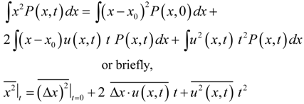
Now we introduce the central argument of the present chapter: we assume, as an emerging result out of the statistics of a vast number of diffusion processes, the complete statistical independence of the velocities
and
, and thus also of
and the positions
:
This is justified considering the statistics of huge numbers, millions of millions of diffusive sub-quantum Brownian motions, which are supposed to bring forth the emergence of said larger-scale collective phenomenon, i.e., the diffusion wave fields as solutions to the heat equation [3]. (In our associative picture, these are nothing but the analogy to the walkers’ Faraday waves emitted with some fixed frequency.) In other words, Equation (8.2.2) represents the effect of collectively “smoothing out” the “erratic” processes of individual Brownian motions. Thereby, the mean convective and diffusion velocities must be unbiased (lest one introduces new physics), and thus linearly uncorrelated. (Note that it was exactly the corresponding average orthogonality of momentum and momentum changes which has led to a first new derivation of the Schrödinger equation [33], as well as the subsequent one based on nonequilibrium thermodynamics [2,3].)
Therefore, with the thus introduced Ord-type projection, i.e., the orthogonality of classical (convective) momentum on one hand, and its associated diffusive momentum on the other, one gets rid of the term linear in
in Equation(8.2.3), and thus of irreversibility, and one obtains
![Entropy 12 01975 i002]()
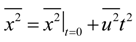
Equation (8.2.5) is the result obtained for the “pure” emergent diffusive motion as given by (8.2.2).
However, in a more realistic scenario, such a smooth diffusive motion will just represent an idealized case, or one, respectively, at very short time scales only, i.e., before some “disturbances” of the surroundings will destroy the said smooth motion. That is, to invoke a more realistic scenario, the smooth behaviour in a completely isotropic and unconstrained environment will have to be substituted by behaviour in an anisotropic, constrained environment. Thus, if we imagine the bouncing of a walker in its “fluid” environment, the latter will become “excited” or “heated up” wherever, in the said anisotropic manner, the momentum fluctuations direct the particle to. After some time span (which can be rather short, considering the very rapid oscillations of elementary particles), a whole area of the particle’s environment will be coherently heated up in this way. (Considering the electron, for example, the fact that it “bounces” roughly
times per second, with each bounce eventually providing a slight displacement from the original path’s momentum, one can thus understand the “area filling” capacity of any quantum path whose fractal dimension was shown to be equal to
. [47])
Now, let us assume we have a source of identical particles, which are prepared in such a way that each one ideally has an initial (classical) velocity
. Even if we let them emerge one at a time only, say, from an aperture with unsharp edges (thus avoiding diffraction effects to good approximation), the probability density
will be a Gaussian one. This comes along with a heat distribution generated by the oscillating (“bouncing”) particle(s) within the constraints of that “Gaussian slit”, i.e., with a maximum at the center of the aperture
. So, we have, in one dimension for simplicity, the corresponding solution of the heat equation,
with the usual variance
, where we shall choose
.
Note that from Equation (8.2.1) one has for the averages over particle positions and fluctuations (as represented via the probability density
)
with the mean values (generally defined in
dimensional configuration space)
As opposed to Equation (8.2.1), where
can take on an arbitrary value such that
is generally variable, equation (8.2.7) is a statement of total average energy conservation, i.e., holding for all times
. This means that in Equation (8.2.7), a variation in
implies a varying “particle energy”
, and vice versa, such that each of the summands on the right hand side for itself is not conserved. In fact, as shall be detailed below, there will generally be an exchange of momentum between the two terms providing a net balance
where
describes a change in the ”convective“ velocity
paralleled by the “diffusive” momentum fluctuation
in the thermal environment.
As elaborated in references [2,3], once Equation (8.2.1) is assumed, considerations based on Boltzmann’s relation between action and angular frequency of an oscillator provide, without any further reference to quantum theory, that
Now we make use of one out of a whole series of practical identities, which Garbaczewski has collected in [37]. (These identities hold true on general information theoretic grounds and are thus not bound to quantum mechanical issues.) Said identity, which can easily be checked by integration, is given by
In a further step, we now introduce a way to prepare for an Ord-type of projection as mentioned in the previous chapter, i.e., to cut out a “slice of time” from an otherwise irreversible evolution as given by the assumed diffusion process. To do this, we shall first combine Equations (8.2.10) and (8.2.11), and shall then insert (8.2.6) for the initial time,
. As from (8.2.7) one has that
and thus also
and as only the kinetic energy varies, one obtains
. Then, with the Gaussian (8.2.6), this provides an expression for the averaged fluctuating kinetic energy, or heat, of a particle and its surroundings,
![Entropy 12 01975 i003]()
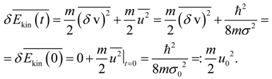
Equation (8.2.12) is an expression of the fact that at the time
the system is known to be in the prepared state whose fluctuating kinetic energy term is solely determined by the initial value
, whereas for later times
it decomposes into the term representing the particle’s changed kinetic energy and the term including
. As the kinetic energy term of the particle increases, the convective velocity becomes
, and, correspondingly,
. In other words, one can decompose said term into its initial
value and a subtracted fluctuating kinetic energy term, respectively, i.e.,
where the last term on the right hand side is identical to
in order to fulfil Equation (8.2.12), and also in agreement with Equation (8.2.9).
From Equations (8.2.12) and (8.2.13) one derives minimal uncertainty relations for all
, i.e.,
![Entropy 12 01975 i012]()
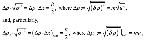
Moreover, with the “diffusion constant”
Equation (8.2.12) provides an expression for the initial velocity fluctuation,
Now we take into account the small momentum fluctuations
from (8.2.13), providing an altered convective velocity
, and thus an additional displacement
i.e., as soon as
. Therefore, in Equation (8.2.2) one now must decompose
into its initial value
and a fluctuating contribution
, respectively. Unless some thermal equilibrium were reached, the latter is typically given off from the “heated” thermal bath to the particle of velocity
,
which is in accordance with (8.2.13)
As opposed to (8.2.2), Equation (8.2.17) now provides the particle’s total displacement
Squaring (8.2.18) provides
Since
one obtains in accordance with Equation (8.2.9) that the last terms on the l.h.s. and on the r.h.s. of (8.2.19), respectively, cancel each other out. Moreover, as the product terms in (8.2.19) are subject to the average orthogonality condition, one obtains through averaging over positions and fluctuations that
![Entropy 12 01975 i004]()
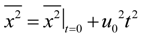
Inserting (8.2.16) into (8.2.20) for the particular case that
(i.e., ), provides for the time evolution of the wave packet’s variance
The quadratic time-dependence of the variance
is remarkable insofar as in ordinary diffusion processes the scenario is different. There, with the Gaussian distribution being a solution of the heat equation, for purely Brownian motion the variance grows only linearly with time, i.e., as described by the familiar relation
![Entropy 12 01975 i005]()
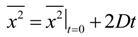
However, as we have seen, the momentum exchange between the particle and its environment is characterized by both a changing velocity and by a changing thermal environment of the particle, i.e., also by a changing diffusivity. Therefore, Equation (8.2.22) must be modified to allow for a time-dependent diffusivity.
In other words, we shall have to deal with the field of anomalous diffusion. This means that instead of the diffusion constant
in the usual heat equation, we now introduce a time-dependent diffusion coefficient
, where
is a constant factor and the exponent
has to be derived upon comparison with Equation (8.2.21). Thus, we write the heat equation in the more general form
and, inserting for
the Gaussian (8.2.6), one obtains after a short calculation that
Integration then provides (with integration constant
)
Upon comparison with (8.2.21) we obtain that
and
which can only be fulfilled by
. Therefore,
, and the time-dependent diffusion coefficient becomes
Note that with the exponent of
being
, or the
-dependence of
in (8.2.21), respectively, one deals with the special case of anomalous diffusion usually named ballistic diffusion. We shall review some general properties of ballistic diffusion in the last chapter. At this point, however, it is useful to recall that throughout the modelling of sub-quantum processes in the present chapter, we deal with various processes at different time scales. On the shortest scales, we have assumed Brownian-type motions (not detailed here), which, on the next higher level of (spatial and) temporal scales lead collectively to the emergence of a regular diffusion wave. The latter is characterized by a velocity
according to (8.2.2), and it is orthogonal on average to the particle’s velocity
, thus providing the r.m.s. displacement (8.2.5) depending on
. As a next step, we have introduced the noisy thermal bath of the particle’s environment, i.e., essentially the effect of other diffusion wave configurations, which disturbs the relation (8.2.5) by introducing a fluctuating term
. The net effect of the latter, however, is the r.m.s. displacement (8.2.20) with a dependence solely on the initial diffusive velocity
. This manifests itself also in the expression for
of the ultimately emerging ballistic diffusion, which is also dependent only on
. However, even on the level of ballistic diffusion one can recover the signature of Brownian motion. In fact, if one considers the time-average of
for large enough times
, i.e.,
one immediately obtains the linear-in-time Brownian relation
![Entropy 12 01975 i006]() which is, however, also in accordance with the
dependence of Equation(8.2.21).
which is, however, also in accordance with the
dependence of Equation(8.2.21).

Note that the diffusivity’s rate of change is a constant,
such that it is determined only by the initial r.m.s. distribution
. In other words, the smaller the initial
, the faster
will change. With the square root of (8.2.21),
we note that
is a spreading ratio for the wave packet independent of
. This functional relationship is thus not only valid for the particular point
but for all
of the Gaussian. Therefore, one can generalize (8.2.31) for all
, i.e.,
In other words, one derives also the time-invariant ratio
Now we remind ourselves that we deal with a particle of velocity
immersed in a wave-like thermal bath that permanently provides some momentum fluctuations
. The latter are reflected in Equation (8.2.31) via the r.m.s. deviation
from the usual classical path. In other words, one has to do with a wave packet with an overall uniform motion given by
, where the position
moves like a free classical particle. As the packet spreads according to Equation(8.2.31),
describes the motion of a point of this packet that was initially at
. Depending on whether initially
or
, then, respectively, said spreading happens faster or slower than that for
. In our picture, this is easy to understand. For a particle exactly at the center of the packet
, the momentum contributions from the “heated up” environment on average cancel each other for symmetry reasons. However, the further off a particle is from that center, the stronger this symmetry will be broken, i.e., leading to a position-dependent net acceleration or deceleration, respectively, or, in effect, to the “decay of the wave packet”. Moreover, also the appearance of the time-dependent diffusivity
is straightforward in our model. Essentially, the “decay of the wave packet” simply results from sub-quantum diffusion with a diffusivity varying in time due to the particle’s changing thermal environment: as the heat initially concentrated in a narrow spatial domain gets gradually dispersed, so must the diffusivity of the medium change accordingly.
In conclusion, then, one obtains with Equations (8.2.32) and (8.2.15) for the “smoothed out” trajectories (i.e., those averaged over a very large number of Brownian motions)
Moreover, one can now also calculate the average total velocity,
Thus, with (8.2.32), one obtains the average total velocity field of a Gaussian wave packet as
Next to the fundamental relations (8.2.29), Equations (8.2.34) and (8.2.36) are the main results of this part of the chapter. They provide the trajectory distributions and the velocity field of a Gaussian wave packet as derived solely from classical physics. Note that the trajectories are not the “real” ones, but only represent the averaged behaviour of a statistical ensemble. The results are in full concordance with quantum theory, and in particular with Bohmian trajectories. (For a comparison with the latter, see, for example, [14].) This is so despite the fact that no quantum mechanics has been used yet, i.e., neither a quantum mechanical wave function, or the Schrödinger equation, respectively, nor a guiding wave equation, nor a quantum potential.
Implicitly, of course, one can easily find the connections to the rhetoric of (Bohmian or other) quantum mechanics. As for the Bohmian case, one just needs to consider the expression for the quantum potential,
Then one has, again with the help of the general relation (8.2.11),
and thus obtains from Equation (8.2.6) for
the time-independent expression for the average quantum potential as
![Entropy 12 01975 i007]()

The expression (8.2.39) is identical to the one we obtained on the r.h.s. of (8.2.12), such that we find that the energy conservation law (8.2.7) can be rewritten as
i.e., where
Still, it is rather remarkable that the results presented above can be arrived at without even referring to (Bohmian or other) quantum mechanics. However, let us now see how a “translation” of the present formalism into that of ordinary quantum mechanics can be accomplished.
It is straightforward to simulate the diffusion process of Equation (8.2.20) in a simple computer model. Using coupled map lattices (CML), one approximates the heat equation as usual by
and for our anomalous (“ballistic”) diffusion one simply inserts (8.2.27) into (8.2.42).
The result is depicted in Figure 1, where the (macroscopic, classical) velocity is chosen as
. (For examples with
and different
, see [48].) Moreover, nine exemplary averaged Bohmian trajectories are shown in Figure 1, and it must be stressed that the Figure shows the emerging behaviour of the Gaussian packet following solely from the CML simulation of Eq. (8.2.42). In addition, the emerging trajectories from the simulation are shown together with the calculated ones from (8.2.34), providing exactly the same trajectories (i.e., up to resolution limits due to discretization).
Note that the trajectories are not the “real” ones, but only represent the averaged behaviour of a statistical ensemble. The results are in full concordance with quantum theory, and in particular with Bohmian trajectories. This is so despite the fact that no quantum mechanics has been used yet, i.e., neither a quantum mechanical wave function, or the Schrödinger equation, respectively, nor a guiding wave equation, nor a quantum potential. Moreover, we want to stress that our model offers possible insights into the sub-quantum domain which must escape (Bohmian or orthodox) quantum theory because the latter simply does not employ the “language” necessary to express them. Note, for example, that the existence of the hyperbolic trajectories depicted in Figure 1, which are given by the formula for the scale invariant wave packet spread (8.2.21), has a simple physical explanation in terms of sub-quantum processes. As the inflection points of the hyperbolas are, according to (8.2.21), characterized by the relation
, i.e., by the length scales
, the trajectories’ evolution is easily understood: as long as the main bulk of the heat “stored” in the initial Gaussian spreads well “inside” the distribution,
, the average particle velocity
is not affected much. However, if said main bulk approximately reaches the distance
, or spreads to regions
, respectively, the particles will “feel” the full heat and get propagated into new directions. For
, then,
becomes the spreading rate of the whole Gaussian packet:
In other words, the “spreading” already begins at
, but becomes “visible” in terms of deflected trajectories only when
.
Figure 1.
Dispersion of a free Gaussian wave packet.

Figure 1: Considering the particles of a source as oscillating “bouncers”, they can be shown to “heat up” their environment in such a way that the particles leaving the source (and thus becoming “walkers”) are guided through the thus created thermal “landscape”. In the Figures, the classically simulated evolution of exemplary averaged trajectories is shown (i.e., averaged over many single trajectories of Brownian-type motions). The results are in full agreement with quantum theory, and in particular with Bohmian trajectories. This is so despite the fact that no quantum mechanics is used in the calculations (i.e., neither a quantum mechanical wave function, nor a guiding wave equation, nor a quantum potential), but purely classical physics. The Figure displays a simulation with coupled map lattices of classical ballistic diffusion, with a time-dependent diffusivity as given by Equation (8.2.27). In the (1+1)-dimensional space-time diagram, both the emerging intensity field and nine exemplary emerging trajectories are shown (dark lines). They exactly match with the superimposed (bright) calculated trajectories from Equation (8.2.34). Note that the emerging hyperbolas’ inflection points occur at the scale
, a fact which has a direct physical meaning: It is there where the main bulk of the heat concentrated within the Gaussian reaches the latter’s average “borders”. Whereas at earlier times the heat was essentially spreading “inside” the original distribution, it now begins to affect the distribution itself by broadening it via heat dissipation.
Figure 2.
Dispersion of a Gaussian wave packet in a gravitational field.

Figure 2: Same as Figure 1, but with the addition of a linear (e.g., gravitational) field. The results are again in full agreement with quantum theory, and in particular with Bohmian trajectories, despite the use of a classical CML simulation of ballistic diffusion, now modified according to the substitution of the classical velocity by
. Again, both the emerging intensity field and nine exemplary emerging trajectories are shown (dark lines), thereby more or less exactly superimposing the (bright) calculated trajectories due to Equation (8.3.3). Note that some trajectories of the dispersing Gaussian even overcome gravity for a well-defined period of time. In fact, our sub-quantum model provides a detailed explanation of why, and within which time limits, this “anti-gravity” effect becomes possible: Some of the upper curves’ extrema occur at the scale
, which describes the maximum of the “anti-gravity” effect, because it is there where the heat of the main bulk of the packet is consumed, which has via the kinetic energy counter-acted the effect of gravity for initial times. For larger times, then, the remaining heat gets gradually less, and therefore gravitational acceleration begins to dominate the trajectories’ curvature.
8.3. Addition of a Linear Potential
So far we have shown that free one-particle quantum motion is exactly identical to sub-quantum ballistic diffusion. This is the basis of a research program that would eventually cover more and more complex situations beyond the case of free motion. As a first simple example, we extend the present scheme to include a linear potential. That is, we place the initial Gaussian packet (8.2.6) in a uniform potential
, which may be an electric or a gravitational field, for example. For illustration, but without loss of generality, we substitute in the following
by
, i.e., we shall discuss a Gaussian packet freely falling due to the potential
.
At this point it is important to note that our derivation of the time evolution of the free packet’s variance, Equation (8.2.21), was based on considerations of variable kinetic energies only. In fact, this must hold true also when a spreading packet is placed into a potential, simply because of momentum conservation and the fact that heat, or kinetic energy, respectively, cannot be transformed into the potential energies envisaged here, and vice versa. (This is therefore a different scenario from the “traditional Bohmian” one, where the “quantum potential” is not considered as a kinetic energy.) Therefore, in our case of ballistic diffusion, relation (8.2.32) still holds, except that now one has to substitute the coordinates
by generalized ones,
, where (in one dimension for simplicity)
Then, with the analogue of (8.2.32),
one obtains the trajectories of particles in a gravitational field in a modification of (8.2.34) as
from which one immediately obtains the particle acceleration
In Figure 2, exemplary trajectories of a Gaussian in a gravitational field are shown as obtained by the CML simulation of ballistic diffusion, modified by the substitution
. The trajectories are superimposed by those derived directly from Equation(8.3.3), and again exhibit excellent agreement.
As noted by Holland [14], one can deduce from Equation (8.3.3) some interesting features of the motion. The most curious one is that the acceleration of a particle of mass
may be greater or less than that of
depending on the size of the mass rates, i.e., in some cases heavier objects may fall more slowly. Of course, a particle at the center of the Gaussian will stay there (because of zero net contributions of the symmetrically distributed surrounding heat) and follow the classical trajectory.
However, note that some trajectories of the dispersing Gaussian even overcome gravity for a well-defined period of time, as can also be seen in Figure 2. In fact, our sub-quantum model provides a detailed explanation of why, and within which time limits, this “anti-gravity” effect becomes possible. A look at the last expression of Equation (8.3.4) provides the answer. Similarly to the discussion of the hyperbolas’ inflection points in the free case, one deals also here with an extremum at the scale
. However, this time the corresponding expression (in rectangular brackets) is antagonistic to
. In other words, said scale describes the maximum of the “anti-gravity” effect, because it is there where the heat of the main bulk of the packet is consumed, which has via the kinetic energy counter-acted the effect of gravity. For larger times, then, the remaining heat gets gradually less, and therefore gravitational acceleration begins to dominate the trajectories’ curvature.
8.4. Ballistic Diffusion: Conclusions and Perspectives
Instead of simply repeating the central results of the present chapter in this Summary, I would like to discuss them from a slightly different point of view. For, it turns out that the main results of this chapter can be derived also with the Ornstein-Uhlenbeck theory, and even simpler at that. Consider again a momentum fluctuation
, for which one can write down a Langevin stochastic differential equation
where
is our damping factor due to friction and
is the random fluctuating force. Rewriting Equation (8.4.1), again in one dimension for simplicity, one has
One notes that on average
due to the random nature of the force
, and due to local equilibrium [2], it holds that
such that one obtains the corresponding Langevin equation’s standard Ornstein-Uhlenbeck solution for
in the form
![Entropy 12 01975 i008]() where the diffusion constant
. As we have derived in Chapter 2 the identity
, Equation (8.4.3) reads as
where the diffusion constant
. As we have derived in Chapter 2 the identity
, Equation (8.4.3) reads as
![Entropy 12 01975 i009]()
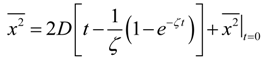
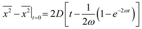
Equation (8.4.4) has two well-known limiting expressions, depending on the choice of the time scale chosen. That is, for
one obtains that
![Entropy 12 01975 i010]() i.e., the description of the usual Brownian-type motion. However, for
, and by expanding the exponential up to second order, Equation (8.4.4) provides that
i.e., the description of the usual Brownian-type motion. However, for
, and by expanding the exponential up to second order, Equation (8.4.4) provides that
![Entropy 12 01975 i011]() that is, exactly our expression (8.2.20) for ballistic diffusion. Note on the one hand, however, that both Equations (8.4.5) and (8.4.6) are approximations holding for specific time scales only. As, on the other hand, from (8.4.6) one derives the usual quantum mechanical formula for the spreading of a free wave packet, one can maintain that the latter is only an approximation, whereas the more exact expression is given by Equation (8.4.4). Moreover, one thing must also be stressed in this summary: throughout the whole chapter, no use is made of the orthodox apparatus of quantum mechanics, or of any alternative ones such as Bohmian mechanics. In fact, only classical physics is employed, which nevertheless provides exact agreement with the corresponding quantum mechanical results.
that is, exactly our expression (8.2.20) for ballistic diffusion. Note on the one hand, however, that both Equations (8.4.5) and (8.4.6) are approximations holding for specific time scales only. As, on the other hand, from (8.4.6) one derives the usual quantum mechanical formula for the spreading of a free wave packet, one can maintain that the latter is only an approximation, whereas the more exact expression is given by Equation (8.4.4). Moreover, one thing must also be stressed in this summary: throughout the whole chapter, no use is made of the orthodox apparatus of quantum mechanics, or of any alternative ones such as Bohmian mechanics. In fact, only classical physics is employed, which nevertheless provides exact agreement with the corresponding quantum mechanical results.
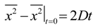
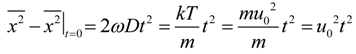
We have shown for the cases of free motion and motion in linear potentials, respectively, that the time evolution of a one-particle quantum system in the noisy heat bath of the surrounding “vacuum” exactly equals that of (classical) ballistic sub-quantum diffusion. Note that there are some well-known general characteristics of ballistic diffusion [49], and the results presented in this chapter agree perfectly with them. For one thing, ballistic diffusion is the only type of diffusion that exhibits reversibility, and because of this it violates ergodicity (i.e., as in our cases). Also, if the ballistic system is not in equilibrium initially, it will never reach equilibrium (which is true here as well). Finally, the result of any measurement depends on the initial conditions. This can be clearly seen also from our results for the time evolution of the Gaussians and the corresponding averaged trajectories, which all depend on the initial values of
, or
, respectively.
9. Conclusions and Outlook
In this review, an extensive discussion was presented of various aspects of a suggested sub-quantum thermodynamics as a basis for emergent quantum theory. On this basis, it has been explicitly shown how the following quantum mechanical features can be derived from purely classical physics: Planck’s relation
for the energy of a particle, the Schrödinger equation for conservative and non-conservative systems, the Heisenberg uncertainty relations, the quantum mechanical superposition principle, Born’s rule, and the quantum mechanical “decay of a Gaussian wave packet”. Moreover, also the energy spectrum of a quantum mechanical harmonic oscillator has been derived classically, as well as that of a “particle in a box”.
Further, it has been proven that free quantum motion exactly equals sub-quantum anomalous (i.e., “ballistic”) diffusion, and, via computer simulations with coupled map lattices, it has been shown how to calculate averaged (Bohmian) trajectories purely from a real-valued classical model. This has been illustrated with the cases of the dispersion of a Gaussian wave packet, both for free quantum motion and for motion in a linear (e.g., gravitational) potential. It has been shown that the results are in excellent agreement with analytical expressions as they are obtained both via our approach, and also via the Bohmian theory. However, in the context of the explanation of Gaussian wave packet dispersion, quantitative statements on the trajectories’ characteristic behaviour were presented, which cannot be formulated in any other existing model for quantum systems.
Concerning the computer simulations, much more should be possible, and we are only just beginning to exploit this simple and practical tool to arrive at classical simulations of “quantum processes”. Of course, as a next step, relative phases will have to be implemented, so as to be able to simulate truly wave-related phenomena such as interference at a double slit, and the like. Moreover, the simulation of interactions with potentials will constitute a major challenge, as well as many-particle processes, or the extension to higher-dimensional scenarios. In principle, however, there is one area where the simulation might prove to have a big advantage, i.e., in situations of high complexity, where the usual analytic tools of ordinary quantum mechanics would be insufficient. In sum, there is a great potential for novelty with our classical simulation approach.
Finally, one must also mention the challenges as given by quantum mechanical nonlocality and the model’s possible relativistic extensions, respectively. The fact that with diffusion wave fields spatial coherence can be created out of random ensembles of diffusive energy is per se already highly interesting. Moreover, as has been pointed out, in this context one needs to mention that the equations of the type (6.2.11) yield “the physical artefact of infinite speed of field propagation, though with vanishingly small amplitude, at remote locations away from the source. (…) Because propagation is instantaneous, the equations yield no travelling waves, no wave-fronts, and no phase velocity. Rather, the entire domain ‘breathes’ in phase with the oscillating source. In the world of diffusion waves, there are only spatially correlated phase lags controlled by the diffusion length.” [50] Naturally, if any phenomena from classical physics should be helpful at all in this regard, these features make diffusion waves particularly amenable for modelling quantum mechanical nonlocality.
One can thus imagine the following scenario for, e.g., an experiment in neutron interferometry. With a prepared neutron source in a reactor, one immediately has a thermal field in the “vacuum” that nonlocally links the neutron oven, the apparatus (including, e.g., a Mach-Zehnder interferometer), and the detectors. The (typical) Gaussians used to describe the initial quantum mechanical particle distributions thus also contribute in their totality to the form of the heat distribution in the overall system, no matter which particle actually is on its way through the interferometer. In this way, all “potential” paths are implicitly present throughout the experiment (i.e., under constant boundary conditions) in that the corresponding thermal field is spread out no matter where the particle actually is. That this can be assumed is, of course, solely due to the fact of the infinite propagation of diffusion wave fields. Moreover, eventual relativistic formulations of the physics of diffusion wave fields would thus become of primary importance.
At last, let me mention that this review is in no way intended to provide a closed chapter of, say, emergent quantum mechanics. On the contrary, as with research in general, a comprehensive view of ongoing research activity is, particularly when devoted to such foundational issues, almost a self-contradictory project per se, because the process goes on as we write or read. One can say that work in the domain of basic research is always work in progress.
Acknowledgements
I sincerely thank my long-time friends and collaborators at AINS, Siegfried Fussy, Johannes Mesa Pascasio, and Herbert Schwabl, for their invaluable contributions and support, and, of course, also for the lots of fun we had, and still have, by being involved in this exciting field of basic research.
References
- Carroll, R. On the Emergence Theme of Physics; World Scientific: Singapore, 2010. [Google Scholar]
- Grössing, G. The vacuum fluctuation theorem: Exact Schrödinger equation via nonequilibrium thermodynamics. Phys. Lett. A 2008, 372, 4556–4563. [Google Scholar] [CrossRef]
- Grössing, G. On the thermodynamic origin of the quantum potential. Physica A 2009, 388, 811–823. [Google Scholar] [CrossRef]
- Grössing, G.; Mesa Pascasio, J. A classical explanation of quantization. arXiv 2010. 0812.3561. [Google Scholar] [CrossRef]
- Adler, S.L. Quantum Theory as an Emergent Phenomenon: The Statistical Mechanics of Matrix Models as the Precursor of Quantum Field Theory; Cambridge University Press: Cambridge, UK, 2004. [Google Scholar]
- Nelson, E. Quantum Fluctuations; Princeton University Press: Princeton, NJ, USA, 1985. [Google Scholar]
- El Naschie, M.S. A note on quantum mechanics, diffusional interference and informions. Chaos Soliton. Fractal. 1995, 5, 881–884. [Google Scholar] [CrossRef]
- Nottale, L. Fractal Space-Time and Microphysics: Towards a Theory of Scale Relativity; World Scientific: Singapore, 1993. [Google Scholar]
- Fritsche, L.; Haugk, M. A new look at the derivation of the Schrödinger equation from Newtonian mechanics. Ann. Phys. (Leipzig) 2003, 12, 371–403. [Google Scholar] [CrossRef]
- Elze, H.-T. The attractor and the quantum states. Int. J. Qu. Info. 2009, 7, 83–96. [Google Scholar] [CrossRef]
- Rusov, V.D.; Vlasenko, D.S.; Mavrodiev, S.C. On the procedure of quantization in classical mechanics and the reality of Bohm's ψ-Field. Ukr. J. Phys. 2009, 54, 1131–1138. [Google Scholar]
- 't Hooft, G. Quantum mechanics and determinism. In Proceedings of the Eighth International Conference on Particles, Strings and Cosmology; Frampton, P., Ng, J., Eds.; Rinton Press: Chapel Hill, NC, USA, 2001; pp. 275–285. [Google Scholar]
- Gell-Mann, M. Questions for the future. In The nature of matter: Wolfson College Lectures 1980; Mulvey, J.H., Ed.; Clarendon Press: Oxford, UK, 1981; pp. 169–198. [Google Scholar]
- Holland, P.R. The Quantum Theory of Motion: An account of the de Broglie-Bohm causal interpretation of quantum mechanics; Cambridge University Press: Cambridge, UK, 1993. [Google Scholar]
- Nelson, E. Derivation of the Schrödinger equation from Newtonian mechanics. Phys. Rev. 1966, 150, 1079–1085. [Google Scholar] [CrossRef]
- Feynman, R.P. QED - The Strange Theory of Light and Matter; Penguin Books: London, UK, 1990. [Google Scholar]
- Feynman, R.P. The Feynman Lectures on Physics 3: Quantum Mechanics; Addison-Wesley: Reading, MA, USA, 1966. [Google Scholar]
- Protière, S.; Boudaoud, A.; Couder, Y. Particle-wave association on a fluid interface. J. Fluid Mech. 2006, 554, 85–108. [Google Scholar] [CrossRef]
- Couder, Y.; Fort, E. Single-particle diffraction and interference at a macroscopic scale. Phys. Rev. Lett. 2006, 97, 154101. [Google Scholar] [CrossRef] [PubMed]
- Eddi, A.; Fort, E.; Moisy, F.; Couder, Y. Unpredictable tunneling of a classical wave-particle association. Phys. Rev. Lett. 2009, 102, 240401. [Google Scholar] [CrossRef] [PubMed]
- Couder, Y.; Protière, S.; Fort, E.; Boudaoud, A. Dynamical phenomena: Walking and orbiting droplets. Nature 2005, 437, 208. [Google Scholar] [CrossRef] [PubMed]
- Coffey, W.T.; Kalmykov, Y.P.; Waldron, J.T. The Langevin Equation: With Applications to Stochastic Problems in Physics, Chemistry and Electrical Engineering, 2nd ed; World Scientific: Singapore, 2004. [Google Scholar]
- Verlinde, E.P. On the origin of gravity and the laws of newton. arXiv 2010. 1001.0785. [Google Scholar] [CrossRef]
- Wallstrom, T.C. Inequivalence between the Schrödinger equation and the Madelung hydrodynamic equations. Phys. Rev. A 1994, 49, 1613–1617. [Google Scholar] [CrossRef] [PubMed]
- Boyer, T.H. Thermodynamics of the harmonic oscillator: Wien's displacement law and the Planck spectrum. Am. J. Phys. 2003, 71, 866–870. [Google Scholar] [CrossRef]
- Gallavotti, G.; Cohen, E.G.D. Dynamical ensembles in stationary states. J. Stat. Phys. 1995, 80, 931–970. [Google Scholar] [CrossRef]
- Evans, D.J.; Searles, D.J. The Fluctuation Theorem. Adv. Phys. 2002, 51, 1529–1585. [Google Scholar] [CrossRef]
- Williams, S.R.; Searles, D.J.; Evans, D.J. Independence of the transient fluctuation theorem to thermostatting details. Phys. Rev. E 2006, 70, 66113. [Google Scholar] [CrossRef]
- Carberry, D.M.; Reid, J.C.; Wang, G.M.; Sevick, E.M.; Searles, D.J.; Evans, D.J. Fluctuations and Irreversibility: An experimental demonstration of a second-law-like theorem using a colloidal particle held in an optical trap. Phys. Rev. Lett. 2004, 92, 140601. [Google Scholar] [CrossRef] [PubMed]
- Boltzmann, L. Über die mechanische Bedeutung des zweiten Hauptsatzes der Wärmetheorie. Wien. Ber. 1866, 53, 195–200. [Google Scholar]
- Brillouin, L. Tensors in Mechanics and Elasticity; Academic Press: New York, NY, USA, 1964. [Google Scholar]
- Goldstein, H.; Poole, C.P.; Safko, J.L. Classical Mechanics, 3rd ed; Addison-Wesley: New York, NY, USA, 2002. [Google Scholar]
- Grössing, G. From classical Hamiltonian flow to quantum theory: Derivation of the Schrödinger equation. Found. Phys. Lett. 2004, 17, 343–362. [Google Scholar] [CrossRef]
- Hall, M.J.W.; Reginatto, M. Schrödinger equation from an exact uncertainty principle. J. Phys. A 2002, 35, 3289–3303. [Google Scholar] [CrossRef]
- Valentini, A. Signal-locality, uncertainty, and the subquantum H-theorem; I and II. Phys. Lett. A 1991, 156, 5–11, and 158, 1–8. [Google Scholar] [CrossRef]
- Bohm, D.; Hiley, B.J. The Undivided Universe: An Ontological Interpretation of Quantum Theory; Routledge: London, UK, 1996. [Google Scholar]
- Garbaczewski, P. Information dynamics: Temporal behavior of uncertainty measures. Cent. Eur. J. Phys. 2008, 6, 158–170. [Google Scholar] [CrossRef]
- Gray, C.G.; Karl, G.; Novikov, V.A. Progress in classical and quantum variational principles. Rep. Prog. Phys. 2004, 67, 159–208. [Google Scholar] [CrossRef]
- Grössing, G. Quantum Cybernetics: Toward a Unification of Relativity and Quantum Theory via Circularly Causal Modeling; Springer: New York, NY, USA, 2000. [Google Scholar]
- Einstein, A. Scientific Papers Presented to Max Born; Oliver and Boyd: Edinburgh, UK, 1953. [Google Scholar]
- Mandelis, A. Diffusion-wave Fields: Mathematical Methods and Green Functions; Springer: New York, NY, USA, 2001. [Google Scholar]
- Becker, R. Theorie der Wärme; Springer: Berlin, Heidelberg, Germany, 1966. [Google Scholar]
- Baker-Jarvis, J.; Kabos, P. Modified de Broglie approach applied to the Schrödinger and Klein-Gordon equations. Phys. Rev. A 2003, 68, 42110. [Google Scholar] [CrossRef]
- Ord, G.N. Schrödinger’s equation and classical Brownian motion. Fortschr. Phys. 1998, 46, 889–896. [Google Scholar] [CrossRef]
- Schrödinger, E. Über die Umkehrung der Naturgesetze. Sitzungsber. Preuss. Akad. Wiss. 1931, 144–153. [Google Scholar]
- Fürth, R. Über einige Beziehungen zwischen klassischer Statistik und Quantenmechanik. Zeitschr. Phys. 1933, 81, 143–162. [Google Scholar] [CrossRef]
- Ord, G.N. Fractal space-time: A geometric analogue of relativistic quantum mechanics. J. Phys. A 1983, 16, 1869. [Google Scholar] [CrossRef]
- Grössing, G.; Fussy, S.; Mesa Pascasio, J.; Schwabl, H. Emergence and collapse of quantum mechanical superposition: Orthogonality of reversible dynamics and irreversible diffusion. Physica A 2010, 389, 4473–4484. [Google Scholar] [CrossRef]
- Vlahos, L.; Isliker, H.; Kominis, Y.; Hizandis, K. Normal and anomalous diffusion: A tutorial. In Order and Chaos, vol. 10, School/Conference Proceedings; Bountis, T., Ed.; Patras University Press: Patras, Greece, 2008. [Google Scholar]
- Mandelis, A. Diffusion waves and their uses. Phys. Tod. 2003, 53, 29–34. [Google Scholar] [CrossRef]
© 2010 by the authors; licensee MDPI, Basel, Switzerland. This article is an open access article distributed under the terms and conditions of the Creative Commons Attribution license (http://creativecommons.org/licenses/by/3.0/).
Share and Cite
MDPI and ACS Style
Grössing, G. Sub-Quantum Thermodynamics as a Basis of Emergent Quantum Mechanics. Entropy 2010, 12, 1975-2044. https://doi.org/10.3390/e12091975
AMA Style
Grössing G. Sub-Quantum Thermodynamics as a Basis of Emergent Quantum Mechanics. Entropy. 2010; 12(9):1975-2044. https://doi.org/10.3390/e12091975
Chicago/Turabian StyleGrössing, Gerhard. 2010. "Sub-Quantum Thermodynamics as a Basis of Emergent Quantum Mechanics" Entropy 12, no. 9: 1975-2044. https://doi.org/10.3390/e12091975