Article

Integrating Post-Processing Kinematic (PPK)–Structure-from-Motion (SfM) with Unmanned Aerial Vehicle (UAV) Photogrammetry and Digital Field Mapping for Structural Geological Analysis

by
Daniele Cirillo
1,2,3,*,
Francesca Cerritelli
4,
Silvano Agostini
5,
Simone Bello
2,3,
Giusy Lavecchia
2,3 and
Francesco Brozzetti
1,2,3
1
Laboratorio di Geologia Strutturale Cartografia e Modellazione Geologica, DiSPuTer, Università G. d’Annunzio, Via dei Vestini, 31, 66100 Chieti, Italy
2
DiSPuTer, Università G. d’Annunzio, Via dei Vestini, 31, 66100 Chieti, Italy
3
CRUST—Centro inteRUniversitario per L’analisi Sismotettonica Tridimensionale, Italy
4
Freelance, Viale Amendola 108, 66020 San Giovanni Teatino, Italy
5
CAAM, Università G. d’Annunzio, Via dei Vestini, 31, 66100 Chieti, Italy
*
Author to whom correspondence should be addressed.
ISPRS Int. J. Geo-Inf. 2022, 11(8), 437; https://doi.org/10.3390/ijgi11080437
Submission received: 7 June 2022 / Revised: 19 July 2022 / Accepted: 28 July 2022 / Published: 2 August 2022

Abstract

:
We studied some exposures of the Roccacaramanico Conglomerate (RCC), a calcareous-clastic mega-bed intercalated within the Late Messinian–Early Pliocene pelitic succession of the La Queglia and Maiella tectonic units (central Apennines). The outcrops, localized in the overturned limb of a kilometric-scale syncline, show a complex array of fractures, including multiple systems of closely spaced cleavages, joints, and mesoscopic faults, which record the progressive deformation associated with the Late Pliocene thrusting. Due to the extent of the investigated sites and a large amount of data to collect, we applied a multi-methodology survey technique integrating unmanned aerial vehicle (UAV) technologies and digital mapping in the field. We reconstructed the 3D digital outcrop model of the RCC in the type area and defined the 3D pattern of fractures and their time–space relationships. The field survey played a pivotal role in determining the various sets of structures, their kinematics, the associated displacements, and relative chronology. The results unveiled the investigated area’s tectonic evolution and provide a deformation model that could be generalized in similar tectonic contexts. Furthermore, the methodology allows for evaluating the reliability of the applied remote survey techniques (i.e., using UAV) compared to those based on the direct measurements of structures using classic devices. Our purpose was to demonstrate that our multi-methodology approach can describe the tectonic evolution of the study area, providing consistent 3D data and using a few ground control points. Finally, we propose two alternative working methods and discuss their different fields of application.

1. Introduction

The study of a fracture system affecting the volume of a rock and the relative chronology between the distinct sets of structures is a “classic” tool used by geoscientists to decipher the tectonic history of a deformed region [1,2]. In sedimentary successions involved in regional-scale deformation zones, the origins and distributions of the different types of tectonic structures are strongly influenced by composition and stratigraphy [3,4]. Lithological heterogeneities (e.g., the alternation of different lithotypes, the variation of bed thicknesses, and cementation) play a primary role in determining the competence of the layers and driving their behavior during the progressive deformation [5]. Some types of rocks are often stingy in providing structural information, for several reasons. They are normally massive and do not contain markers useful to highlight the deformation. Moreover, they are widely vegetated, covered by colluvial deposits, or are affected by widespread landslides. This is the case with poorly consolidated pelitic–arenaceous successions, which frequently occur in the footwalls of major thrust faults in Italy’s northern and central Apennines (e.g., Mts. Sibillini and Gran Sasso Thrust [6,7]).
The study case, regarding the Messinian–Early Pliocene Maiella Flysch underlying the imbricated Mt. Morrone and La Queglia Thrusts [8,9], represents one of such unfavorable frameworks. In fact, no good quality exposures of the flysch-type deposits have been surveyed close to the thrust plane over tens of km.
Luckily, the outcrop here studied was suitable for the structural analysis because it included an 8 m-thick high-competence calcareous–clastic horizon, which recorded the deformation events. This calcareous layer, interbedded within a mostly pelitic succession, consisted of a conglomerate referred to as Roccacaramanico [10,11], San Valentino [12,13], or Sphaeroidinellopsis conglomerate [14,15].
The Roccacaramanico conglomerate (hereinafter referred to as RCC), in addition to being useful for structural analyses and tectonic reconstruction, is extraordinarily suitable for carrying out a study that integrates the methodologies of digital field mapping with those of the photogrammetry using unmanned aerial vehicles (UAVs) and the post-processing kinematic (PPK) analysis.
In this study, we:
  • Performed a detailed structural analysis aimed at characterizing the state of fracture of the RCC and defining the time–space relationships among the various sets of fractures;
  • Made inferences (based on the structural analysis) on the progressive deformation history of the Mio-Pliocene Maiella succession in the context of the Late Pliocene thrusting of eastern Abruzzo;
  • Demonstrated the usefulness of high-resolution photogrammetric methods applied to structural geology to reconstruct a high-resolution 3D digital outcrop model (DOM) and obtain speedily large structural datasets;
  • Tested the applied methodologies and compared the digital and photogrammetric survey results, evaluating and discussing the pros and cons of both methods. Concerning this latter point, we provided a methodological workflow for using UAV technology in combination with digital survey devices (e.g., tablet computers and smartphones), calibrating and checking on the quality of the methods with classic devices.
The use of digital devices is changing the use of traditional approaches in all environments of applied geosciences, such as gradually replacing paper maps with electronic formats. In recent years, geoscientists have developed different field approaches to better manage field activities and workflows for data acquisitions, especially for structural–geological mapping in various geological contexts [16,17,18,19,20,21,22,23,24,25,26,27,28,29]. One of the most valuable digital developments for field surveys involves apps being installed on smartphones and tablets equipped with accelerometers, gyroscopes, magnetometers, and GPS, which are used by the apps themselves to record surface attitudes, such as fault planes and bedding planes or discontinuities in a georeferenced environment. In addition, recent improvements in structure-from-motion (SfM) techniques and small UAVs equipped with onboard GNSS antennas have allowed geoscientists to study outcrops at a sub-meter scale resolution and improve their knowledge of dynamic processes involving them [17,30,31,32,33,34]. Finally, photogrammetry techniques allow, by using the appropriate software, the construction of digital surface models (DSMs), and digital outcrop models (DOMs, also called “virtual outcrop models”) to apply structural geology analyses.

2. Materials and Methods
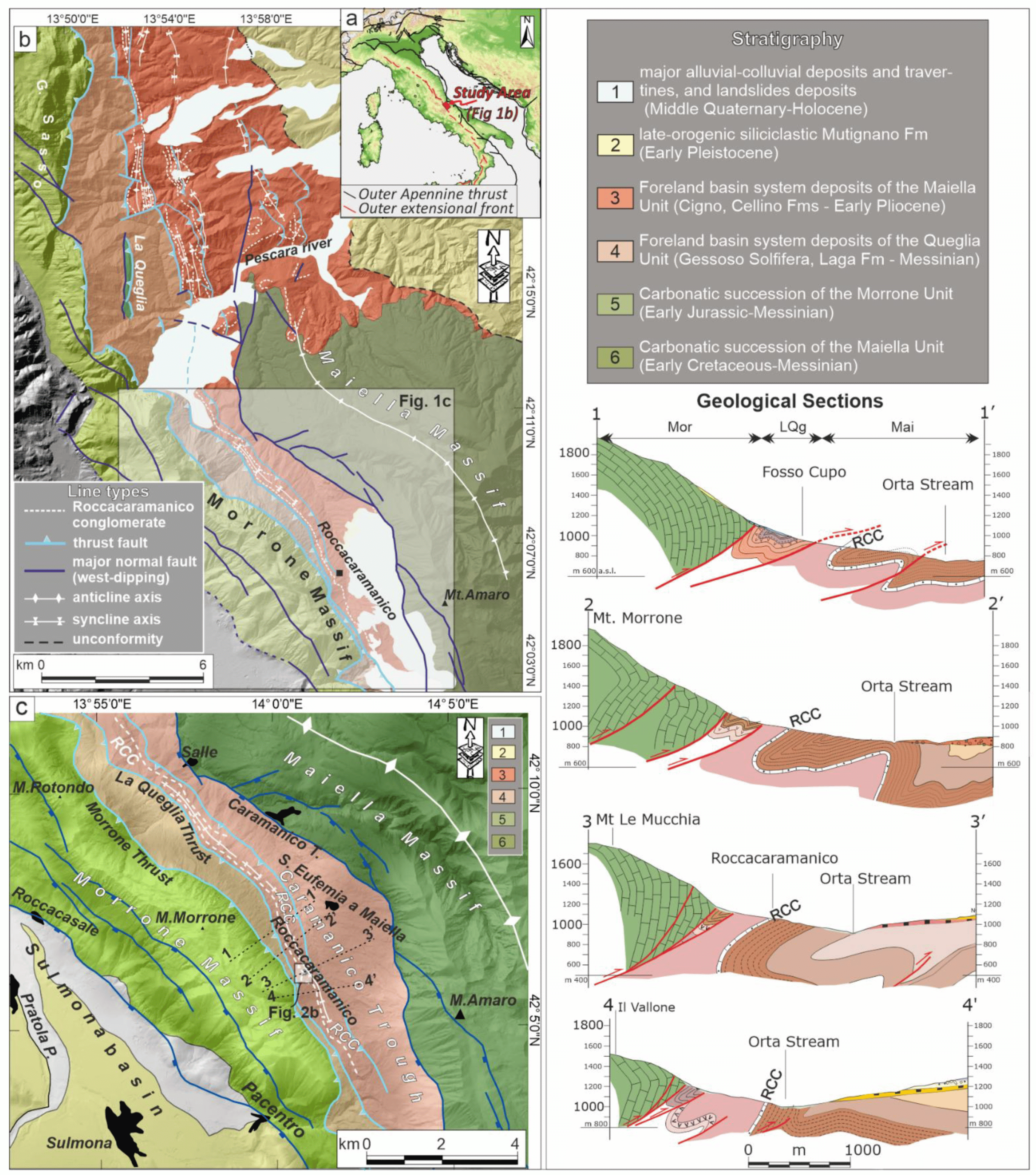
2.1. Study Area

The Central Apennines fold–thrust belt originated from the Neogene–Quaternary tectonic contraction of the western margin of Adria Plate [14,35,36,37,38]. The paleogeographic domains involved in the orogenic deformation are two Triassic–Miocene carbonate platforms, the Latium–Abruzzi and Apulian platforms, and the interposed eastern Marsica–Molise pelagic basin [36]. Presently, the front of the chain is buried below the Padano–Adriatic–Bradanic depression. It was structured during the Late Pliocene–Early Pleistocene, and according to recent works, it is still active [39,40,41,42,43].
The study area is located near the more external intermountain Quaternary extensional belt of Italy that consists of both high-angle (west-dipping), normal, and normal-oblique faults that cross-cut and offset the Mio-Pliocene fold–thrust structures and control the continental basin growth and earthquake activity [27,43,44,45,46,47,48,49].
The study area is located in the eastern Abruzzi Apennines and includes three main tectonic units, all derived from the dissection of the Apulian Platform. From west to east (i.e., from the uppermost to the lowermost), they are the Morrone, La Queglia, and Maiella Units. The Morrone Unit consists of Jurassic–Late Miocene shallow water limestones, passing upward to Messinian evaporites and unconformable wedge-top clastic deposits of the Early Pliocene age. The La Queglia unit crops out with Cretaceous–Messinian ramp carbonates [50,51] followed by Messinian gypsum (Gessoso Solfifera group) and Late Messinian turbidites (La Queglia Flysch [14] or a post-Evaporitic Laga member [13]).
The Maiella Unit, to which the studied outcrops belong, shows a more complex stratigraphic evolution that deserves to be described in depth. During the Mesozoic, the sedimentation was influenced by a ~W–E-striking platform margin. As a result, shallow water limestones characterize the Southern and Central Maiella, whereas the northern sector is characterized by slope and basinal facies [52,53,54,55]. At the end of the Late Cretaceous, the drowning of the platform led to the setting, over the whole area, of a carbonate ramp—a proximal basin environment [56,57,58], which lasted up to the Early Messinian. In these conditions, the Santo Spirito and Bolognano formations were deposited.
The Middle–Late Messinian sedimentation was ‘testified’ by the Gessoso Solfifera group, which includes a pelite interval deposited during the Lago-mare event (Congeria Marls [14], and Lago-Mare Clays [15,59]). The Late Messinian–Early Zanclean boundary, is observed at the base of the Taranta Clays, which includes (1.5 m above the basal boundary) the RCC conglomerate [11,15,60]. In the Maiella Unit, the onset of the Maiella Flysch (also Lama dei Peligni Flysch [61] or Cellino Fm [13]) occurs 180 m above the RCC. The lower turbidite age is referred to as the G. margaritae Biozone, whereas the topmost ones contain bio-assemblages testifying to the G. puncticulata Biozone [13,14,15].
Our study area is located on the western border of the Maiella Unit, near the Roccacaramanico village, in the footwall block of the La Queglia thrust (Figure 1a–c). This latter, in turn, underlies the Morrone thrust, cropping out a few hundred meters to the west. The two thrusts described above are not exactly co-axial. Thus, their traces gradually converge from north to south and nearly overlap. Therefore, the outcrops of the La Queglia unit are very narrow in the Roccacaramanico area. The 3D geological model (Figure S1b) and the geological cross sections (1–4 of Figure 1) show the structural setting of the Maiella Unit, just below the La Queglia thrust. It consists of a syncline–anticline pair, verging to ENE, both showing a tight profile and a 20–30° interlimb angle. The short wavelengths of the folds suggest that they involve only the topmost part of the succession, namely the evaporitic-siliciclastic formations detached from the underlying upper Miocene carbonates. The reverse limb of the syncline (Figure 1, Sections 1–4) consists of the Messinian terms (Gessoso Solfifera and Lago-mare clays), the RCC, the Taranta clays, and the Early Pliocene Maiella Flysch.
In the footwall of the La Queglia thrust, along with the overturned limb of the anticline, the clayey formations that embed the RCC are poorly outcropped and are affected by widespread phenomena of shallow and deep instabilities. Despite allowing to measure the bed attitudes, the few narrow mapped exposures prevent carrying out in-depth geological observations.
Conversely, the Roccacaramanico outcrop of RCC, arranged in reverse polarity a few tens of m below a major thrust surface (Figure 1 and Figure S1), is optimal for performing a structural geological analysis aimed at reconstructing the deformation events that it suffered during the contractional phase.
The serial geological sections of Figure 1 show the structural style that characterizes the sector between the Morrone thrust and the Maiella anticline and allows framing of the analyzed outcrops in the regional tectonic framework of the eastern Abruzzo Apennines.

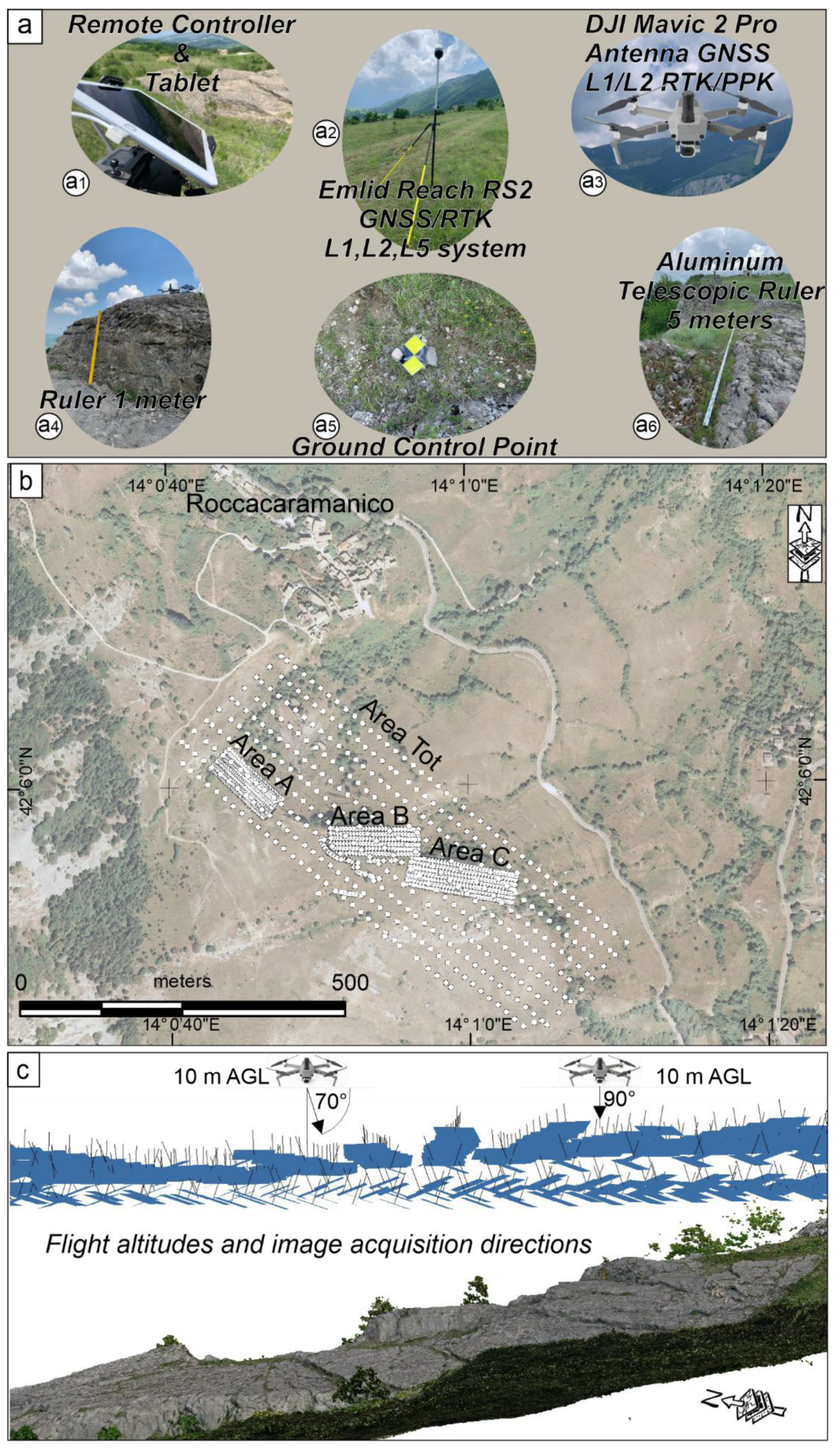
2.2. Global Navigation Satellite System (GNSS) and UAV PPK Fieldwork

The PPK is an alternative technique to the classic photogrammetric survey, acquiring images without positioning ground control points (GCPs). The PPK automatically geo-references the images at the centimeter-scale resolution and does not require a direct correction between the base station and the rover. The base station we used was an Emlid Reach RS2 GNSS/RTK L1, L2, L5 system (Figure 2(a2)); it was positioned on the ground, while the antenna rover (L1/L2 RTK/PPK) was installed on a DJI Mavic 2 Pro drone (Figure 2(a3)) recording raw logs and Rinex files. GNSS Rinex files were then processed to obtain an accurate positioning track of the pre-established flight path.
To pre-set the flight missions, we used the Pix4D app installed on the Apple iPad Air 2 (Figure 2(a1)). Then, we organized the surveys in different aerial paths in automatic flight mode and flew at different altitudes for each outcrop (see Table 1). To obtain a higher resolution of the outcrops, we also carried out manual flights at 3 m a.g.l.
As for automatic acquisitions, we shot the images perpendicular to the flight direction and with an oblique-oriented camera at an incidence angle of 70° (Figure 2c). For the detailed aerophotogrammetric survey (i.e., areas A, B, and C in Figure 2b and Figure S2), the images were acquired in two aerial strips perpendicular to each other, with the camera oriented at 70° and perpendicular to the outcrop. As a result, we acquired 1820 images, with minimal front-lap and side-lap overlapping for 75%.
The subdivision of the entire studied outcrop (area Tot, Figure 2b) into the three areas A, B, and C, in which the RCC shows significant attitude variations was chosen to verify whether bedding variations influence the reciprocal spatial relationships between the multiple sets of structures.

2.3. Preprocessing and Photogrammetry

We first manually selected the UAV images, eliminating those blurred or acquired by mistake (e.g., takeoff). Before uploading the images acquired in the Agisoft Metashape Pro software package to build the digital elevation models (DEMs), orthomosaics, and point clouds, we corrected the geolocations of the shooting points through Toposetter 2.0 PRO. This is an easy-to-use software for automatic GNSS data post-processing and image geotagging that replaces navigation coordinates in EXchangeable Image File (EXIF) tags of images with exact coordinates obtained after post-processing GNSS data.
We constructed DOM, DEMs, orthomosaics, and hillshade reliefs for areas A, B, C, and ’Area Tot’ (Figure 2b, Figure 3 and Figure S2). The quality and details of the products are presented in Table 1.
We used dense point clouds in CloudCompare software (version 2.12 alpha) to acquire new measurements on the virtual outcrops [17,30,31,33,62,63]. In addition, CloudCompare facilitates the 3D surveying of entire rock volumes and new measurement acquisitions with the “Virtual Compass” tool [64], a plugin that we used to measure beddings, joints, and faults that we exported as .csv file formats for the analyses with OpenStereo and FaultKin 8 software [65].
We also used the GeoTrace tool in the QGIS platform to rapidly extract structural features (e.g., joint trend and fault strike), using high-resolution orthomosaics as a base map. Applying this plugin, we measured 2650 features for area A, 1310 for area B, and 1090 for area C. Furthermore, the plugin returns the features in shapefile format (polylines; .shp), which we used to compute the orientations using the QGIS field calculator, and finally plotted as directions on the rose diagrams.

2.4. Digital Survey

In the field, we used Fieldmove Clino and Fieldmove apps, installed respectively on an iPhone (Figure S13a–c) and iPad (Figure S13d–i) to measure the attitudes of different geologic planar and linear features. The former included beddings, cleavages, joints, and faults, while the latter included slickenlines and intersection lines between various planes. First, slickenlines were collected, specifying wherever possible, the sense of slip, providing a kinematic classification of the faults and shear planes (normal, reverse, and strike–slip).
For quality control, before the fieldwork, we exported the orthomosaics obtained from photogrammetry as images (.Geotiff file format), imported them on Move Software (they were saved as .mbtiles), and then we uploaded them on the Fieldmove app. This significantly improved the base map images and the accuracy in positioning the measurements (Figure S13d–f).
As for the accuracy in collecting the data using a digital device, we randomly compared the measurements with those acquired with an analogic compass. After several measurements, we verified errors ranging in the 0–3° interval, which we consider acceptable, in accordance with most of the literature [17,20,66,67].

2.5. Structural Survey

We performed the structural analysis according to classic criteria for the mesoscopic study of fold-and-thrust systems, measuring bedding (b), cleavage (c), joints (j), and faults (f) (Figure 4a).
  • According to the scientific literature [68,69], we use some geological terms as specified—cleavage: closely-spaced systematic fractures generally confined within a single layer. In association with folds, spaced cleavage was distinguished in two sets (Figure 4b): (i) axial plane cleavage when near parallel or convergent to the axial surface, with intersection lineation between the axial plane cleavage and bedding parallel to fold hinge; (ii) transecting (or transversal) cleavage when near orthogonal to the fold hinge. Depending on lithology (carbonatic versus clastic), the axial plane cleavage may present (or not) pressure solution features. The coarse-grained clastic nature of the studied outcrops does not favor pressure solution processes;
  • Joints: high continuity systematic fractures, filled with cement or not, which extend within a series of layers without appreciable offset;
  • Shear planes: minor systematic displacement planes with no fault zone/breccia since the kinematics observed on the shear planes are substantially coherent with those that characterize the adjacent faults; these structures were statistically treated together;
  • Faults: discontinuity planes with significant displacement (i.e., having an order of magnitude comparable to that of the size of the structure), even in the absence of a well-developed breccia.
Figure 4. (a) Example of the bedding–joint plane observed in area A. The red polygons highlight the normal fault planes. (b) Details of the fracture cleavage sets (located in panel (a)).
Ijgi 11 00437 g004
The data acquired in the field and the data extrapolated with the virtual compass tool from the dense point cloud were represented and analyzed with FaultKin 8 software.

2.6. Workflow

To summarize the workflow adopted in this work, we present a synoptic diagram in Figure 5, starting from aerial photogrammetry data acquired in the field. First, the corrections of the geolocalization of the images were modified through high-performance computers and dedicated software for the post-processing kinematic analysis (for more details, see Section 2.3 and Text S1 in the Supplementary material). After this first phase, the images with the corrected coordinates were used through Agisoft Metashape professional software to create the 3D digital outcrop model.
The workflow is divided into two distinct methodologies. The first concerns the FieldMove app, which allows acquiring new data from high-resolution images created through Agisoft Metashape. The second method allows extracting geological data directly from the virtual surfacing model.

3. Results

The studied outcrop (‘Area Tot’ in Figure 2) corresponds to a portion of the RCC in overturned polarity at the footwall of the La Queglia and Morrone thrusts (Figure 1 and Figure S1b,c). It extends 0.5 km along the strike in the average NW–SE direction, with local bending. It was subdivided into three areas (A, B, and C in Figure 2, Figures S1 and S2), each homogeneous in the average attitude and structural setting. We analyzed the structures separately in the three areas, considering area A (Figure 6 and Figure 7) as the key for subsequent interpretations.
Area A is the largest exposure of RCC; therefore, its survey allows a more complete and representative sampling of its fracturing. Furthermore, in A, the bedding attitude is more regular than in B and C (Figure 6 and Figure 7), and the average RCC strike is nearly sub-parallel to the surface trace of the overlying thrusts.
The stratigraphic interval that crops out at A corresponds to the base of the RCC layer, which, due to its cementation and textural characteristic, is particularly rich in well-preserved tectonic structures.
We divided the outcrop of area A into six sectors (I to VI in Figure 7a) separated by the major planar discontinuities (Figure 4). These latter correspond to decametric-scale faults, shear planes, or joints, which seem to have played as local boundaries to fracture development and propagation. In other words, they compartmentalized the deformation. Areas B and C (Figure 7b) are nearly 200 and 320 m SE of area A and can be described together because they provided similar results.

3.1. Measurements and Models Accuracy

Many studies have tested UAV photogrammetry with onboard GNSS RTK/PPK for photogrammetry (e.g., [70,71,72,73,74]). Integrating a PPK GNSS module on a UAV allows the reconstruction of highly detailed DEMs even without placing many GCPs [73,75,76,77] (see errors of the camera locations in Table 2, Text S1, Figures S3–S8). In agreement with the existing literature [73,74,75,77,78], our investigations show that using few GCPs, positioned either in a lateral or central position with respect to the aerial missions, can lead to accuracies of up to 3 cm on GCPs.
We evaluated the accuracies of the GCP/checkpoints calculating standard deviations in individual coordinates X, Y, and Z. According to the expected GNSS PPK measurement accuracy, the results confirm a standard deviation ranging between 3 and 6.9 cm for each GCP measured (see Figure 6).

3.2. Field Structural Analysis

The data collected through the digital survey in areas A (sectors I to VI), B (sector VII), and C (sector VIII) and their stereoplot representations are reported in Figure 7. Different colors of bed planes indicate the different sectors labeled with a number, from 1 to 6, southward. The same label is reported on the stereoplots, which shows the data collected on bedding (b), cleavage (c), joints (J), and faults (f). The shear planes, showing small displacements and no cataclastic flow, clearly result from reactivation of pre-existing fracture cleavages or joints. For this reason, in the graphic representation phase, they were included in the corresponding stereoplot.
From the analysis of the above data, we obtained the following outcomes:
  • From sectors I to VI, the bedding changes dip directions from NW to SW (compare stereoplots b1 to b6, in Figure 7a), which highlights a secondary folding or bending of the overturned RCC layer, due to dragging close to a dextral strike–slip fault;
  • The most numerous brittle fractures, including meter-scale faults and joints, show an average NW–SE trend (Figure 7a, stereoplots j3–j4). This latter results parallel to the main bedding direction in the central–southern portion of the outcrop (sectors IV–VI) and does not seem to be influenced by the bed rotation in the northern portion (sectors I–III); local deviations from the main trend (towards NNW–SSE or WNW–ESE strikes) do not appear to be ubiquitous or have local importance. Finally, a numerically subordinate NE–SW striking joint set is also observed;
  • In all the I–VI sectors, a NE–SW oriented set of the spaced fracture cleavage is well detectable (Figure 7a, stereoplots c2 to c5); this fracture set, despite a certain dispersion (20° in strike), is nearly orthogonal to the bedding strike in the southern sectors (sector IV to VI), whereas it becomes almost parallel to the strike of strata in the northern sectors, where the bedding dips NW-ward (sectors I–III);
  • The major SW dipping fault (i.e., fault f1, which binds the westward sectors III and IV of area A) displays normal kinematics associated with a minor oblique-sinistral component; other significant faults are oriented N–S to N10E, nearly parallel to a minor group of joints of the j3 plot.
Moving from area A to areas B and C, and further to SE, the RCC appears to be deformed in a series of S-shaped blocks, separated by the NE–SW trending dextral strike–slip or oblique-slip faults (Figure 7b). The presence of indicators, such as slickenlines and calcite steps on the faults planes, well constrain the kinematics (Figure S13j). In particular, the RCC outcrop shows a sharp bending around a sub-vertical axis, reaching abruptly a dip direction varying from N 190° to N 165° (Figure 7b, stereoplot b7). The dip direction of the bed results is nearly orthogonal to the traces of the Morrone and La Queglia thrusts and the related macro-folds. The dip angle also changes significantly, ranging from 35° to 70° (Figure 7b). The survey of fractures also highlighted widespread sets of joints and fracture cleavages. Systematic joint sets, following two main trends, sub-parallel and sub-orthogonal to the bed strikes, and transecting fracture cleavages, are well developed in area B (Figure 7b, stereoplots j7 and c7). A peculiarity of area C is the coexistence of diffuse and well-developed cleavage, both parallel and orthogonal to the direction of bedding.
The spatial distributions of the fractures surveyed in areas B and C show that they maintain the same relationships detected in area A with respect to the bedding.

3.3. Structural Analysis of Virtual Outcrops

An example of the structural data acquired with the Virtual Compass tool in CloudCompare is given in Figure 8. The reconstruction of the various structures in area A is shown in Figure 9a–c while the stereoplots in Figure 9d–i, Figure 9j–o, and Figure 9p,q refer to bedding planes, joints, and faults, respectively. Figure 9c also reports the localization of the portion of area A where the data shown in each stereoplot have been measured. Figure 10 represents details of the same outcrop where two systems of joints and cleavage were particularly well developed and deserved to be analyzed in depth. Finally, Figure 11 provides an overview of the entire Roccacaramanico outcrop, including areas A, B, and C.
The outcomes of the “virtual” structural analysis performed on the elaborated DOM can be resumed in the following explanation. In area A, a change of orientation of the bedding planes is highlighted, comparing the northern portion of the outcrop (stereoplots of Figure 9d–f) where the dip direction varies from N 336° to N 300°, with its central-southern portion (stereoplots of Figure 9g–i), where dip direction ranges between N 270° and N 220°. In the entire area, the more evident observable fractures belong to a systematic joint set that shows an average NW–SE direction (both NE and SW dipping, stereoplots of Figure 9m–o) but a certain number of N–S sets also occur (Figure 9j–k). The attitudes of two major faults and some shear planes are characterized by the SW dip direction (i.e., N 235° and N 226°, stereoplots of Figure 9p,q), substantially co-axial with the prevailing joint set.
A well-developed and regularly-spaced set of fracture cleavage, trending NE–SW is widespread in the northern sectors of area A (Figure 4b and Figure 6a sector III); however, the obtained attitudes appear somewhat scattered regarding both dip direction and dip angle (Figure 10 stereoplots e, g, i). Within the cleavage population of area A (Figure 10e), a NW–SE trending set is also represented, which is nearly co-directional with the bed strike. This set, although numerically subordinate, can be interpreted as representative of an axial plane cleavage associated with folding. Based on this assumption, its intersection with strata (L 1-0 lineation) would provide the local axial trend (low angle, NW-dipping) of the recumbent fold of which this outcrop is part (Figure 1, Section 3–3’). From an in-depth analysis, it is evident that the scattering of the NE–SW trending cleavage set is due to secondary deformations; Figure 10a,b highlight that the cleavage surfaces have been locally rotated in cm-scale domino-like systems. Dominoes show a maximum displacement and rotation within dm-to-m scale zones bounded by overlapping extensional shear planes (stepover) showing normal, left oblique kinematics (Figure 10a,b). Figure 11a highlights that a series of NE–SW trending dextral strike–slip faults interrupt the continuity of the RCC in the zones of separation between the three areas. These faults dissect the layers in portions having different bed attitudes (see symbols and stereoplots of Figure 11a–d). The observation above provides chronological constraints to the deformation phases that affected the RCC, with the strike–slip deformation after the folding phases. Analyzing the distribution of the joint orientation in the three areas, A, B, and C (rose diagrams of joint directions in Figure 11b–d), and comparing them with the bedding attitudes (stereoplots of Figure 9d–i, Figure 10d and Figure 11a), we observe that the angular relationships between the major joint sets and the bedding remained constant. In fact, in each area, we detected a main joint set that was nearly co-directional with the bedding and a secondary set making an acute anticlockwise angle with the bed direction. Moreover, a set of low-continuity joints and the fracture cleavage locally occurs orthogonally to the bed direction.

4. Discussion

Our work contributes to two different aspects (particularly regarding geological investigations) in orogenic areas: (1) understanding the brittle deformations affecting a competent layer packed within an incompetent matrix and (2) the evolution of survey methodologies, as the available technological tools become more advanced, faster, and precise. These aspects were complementary since the advancements in mapping techniques directly impacted the quality and number of data collected, which, in turn, influenced the outcome of the research.

4.1. Deformation History and Tectonic Evolution

By deciphering the deformation pattern that characterizes the RCC layer, we reconstructed the tectonic history of the Maiella Messinian–Early Pliocene succession and framed it into the orogenic phase that affected the external Abruzzo Apennines.
This contractional history started during the topmost Early Pliocene and likely extended well into the Late Pliocene. This time span was constrained by the age of the syntectonic deposits of foredeep and wedge-top basins widely documented in the literature [13,14,15,36,61]. As for the rest of the Apennine fold-and-thrust belt, the compressional phase was organized into two major stages: folding (first) and later thrusting and associated strike–slip transfer faulting [79].
During the folding stage that affected the RCC, smaller-scale fractures originated before the thrusting-related limb-overturning, including the two sets of fracture cleavage, orthogonal and perpendicular to the bedding. Of the two sets, the one that was more represented and more regularly spaced was transversal to the axial direction of the fold (~90°), which was reconstructed in the field along the studied portion of the Caramanico Trough (continuous white line in Figure 1c). The other set, whose direction was sub-parallel to the folding axis, and represents the axial plane cleavage, was instead unusually poorly developed, possibly because of the clastic nature of the RCC layer and the very shallow deformation conditions, which both do not favor the pressure solution processes associated with axial plane flattening.
The above reconstruction is based on the early origins of the two cleavage sets that maintain constant angular relationships with the bedding surface, whatever its attitude.
The main folding phase buckled the RCC before the emplacement of the La Queglia thrust. The geometry of the former fold, hypothesized in Figure 12a, is speculative. It cannot be observed in the study area due to its dissection during later thrust faulting. In the surrounding areas (e.g., in the Brittoli–Pietranico area, north of the Pescara Valley, Figure 1a), folds that deform the same succession in an analog structural position of the studied outcrop are marked asymmetrical with a tight transversal profile, but they rarely have overturned limbs with dip angles < 60–70°. In the Roccacaramanico case, the present dip angle of the RCC (locally < 20°) indicates a strongly recumbent geometry that we explain with the protracted and intense shear strains that the layer suffered due to the proximity of the overlying La Queglia thrust (Figure 12c).
Progression of folding generated a typical joint system consisting of transversal and longitudinal sets (Figure 7a(j3,j4) and Figure 12b) with directions perpendicular and sub-parallel, respectively, to the fold axis and of the two diagonal sets, oblique to the fold axis (Figure 7a(j3) and Figure 12a,b).
The genetic connection between the joint system and the main folding phase is suggested primarily by the typical pattern, similar to those recognized in many fold belts worldwide ([80] and references therein). Moreover, it is confirmed by the observation that, moving from area A to areas B and C (Figure 11b–d), all the joint sets rotate together as the direction of the plicative structure rotates (details in Section 3.3).
As shown in the geological cross sections of Figure 1, the thrusting of the La Queglia and Morrone units caused an intense deformation of the Maiella terrigenous succession involved in a regional-scale east-verging shear zone. However, due to its stiffness and competence, the RCC mainly experienced brittle behavior.
The main effects of this later thrust stage were the diffuse reactivation of the pre-existing fractures that were favorably oriented to the strain field (Figure 12b). In particular, the westward dipping longitudinal joints were prone to be reactivated as extensional shear planes or mesoscopic faults (e.g., the stereonet f1, and f3 in Figure 7), with some meters associated with displacement. The extensional kinematics of these structures (Figure 8b) could seem surprising in a contractional context, but it was functional to accommodate the stretching and thinning of the overturned limb. Furthermore, the pre-existing axial plane cleavage attitude justifies its reactivation as antithetical Riedel planes, with respect to the spatial orientation of the thrust plane (Figure 12c).
Both the extensional meso-faults and shear planes produce an effect of stretching and layer-parallel flattening of the RCC that is, to all effects, compatible with the top-to-east sense of shear to which the layer was subject during the thrusting stage (Figure 12c).
In this perspective, the slight oblique movements recorded on the fault plane f1 (Figure 7a–c) could be related to a certain strike–slip component of slip (right-lateral?) associated with the movement of the hanging wall during the thrusting phase.
A further peculiar feature, referring to the latest stage of thrusting, is the reactivation of the transversally-oriented cleavages as rotational shear planes delimiting domino-like lithons (details in Section 3 and Figure 10a,b).
The superposition of dextral N 045° to N 060°-oriented strike–slip faults to the folded and sheared RCC can be a further and final stage of the fold-and-thrust deformation phase. These faults dissect and drag the layer originating a series of hectometer scale S-shaped rock bodies whose geometries are coherent with the sense of movements associated with these faults (Figure 11a and Figure 12d). This observation confirms that, according to what was observed in many other zones of the northern–central Apennines [81,82], the strike–slip deformation postdates the folding and develops during the final thrusting phases.

4.2. Comparison between the Methods Used

A heated debate is taking place within the geological community on the advantages and limits of the field mapping techniques supported, to varying degrees, by advanced technologies.
Our work, aimed firstly at solving a classical structural geological problem (unveiling the succession of tectonic events that affect a region), allowed us to test two alternative methods of performing a “new generation” structural survey. Refer to Section 2.2, Section 2.3, Section 2.4 and Section 2.5 for technical descriptions of these procedures and their accuracies.
Method 1 implies greater work, both in the field and in the laboratory, and requires: (1) an initial acquisition and elaboration of UAV-shot images to obtain good quality georeferenced orthomosaics of the outcrop, (2) the uploading of such images in hand-portable devices (smartphones or tablet computers) to use as the base map, and (3) the direct measurements in the field of all recognizable features, using devices with the appropriate software.
Method 2 requires a greater number and more detailed imagery acquisitions (UAV flights at different heights) needed to reconstruct a high-resolution virtual outcrop, which, by means of dedicated applications, performs the structural analysis in the lab.
In particular, the acquisition of many images from low-altitude flights (a few meters above the outcrop surface) and long processing times are necessary to apply this second method.
In Table S1, we show the results obtained by applying the two methods. The main differences are the number of data acquired in the field with the FieldMove app and the data extracted from the CloudCompare software.
The higher discrepancy measured regards the slickenside’s attitude on Fault 2 (F2), for which it reaches 25°. This is due to the different number of data acquired with the two methods, the bending of the fault along the strike, and the impossibility to collect data at the same location.
The fields of application of the two methods may depend on the type of work to be conducted. In the presented case, where the main aim was to achieve the best possible understanding of the geological history of the study area, which had no strict time limits, both were applied as complementary and consequential parts of the same investigation process to be progressively deepened.
In other cases, they could be used separately, selecting the most functional method for the specific targets of the work. In particular, the type and completeness of the expected dataset, the quality and extent of the outcrops, and their accessibility, could be considered elements of choice.
Depending on the project, data collection via UAV may offer several advantages because of its capabilities to capture low-altitude imagery and process data using automated SfM image measurements.
Although there are several advantages, there are disadvantages as well to using this evolving technology. Due to weather, regulatory restrictions, and environmental factors, UAVs can be limited in their application. Table S2 shows a list of some of the “Pros” and “Cons”.

5. Conclusions

Our multi-methodology survey of the RCC, integrating UAV technologies and digital field mapping, allowed us to reconstruct the deformation history of a key area of the central Apennines and, at the same time, compare some working techniques that are often considered as alternatives.
In conclusion, we summarize the used procedures in the following two main points.
  • The first method allows a greater ability to select the data by the operator, who can directly examine and check the characteristics of the structures on the outcrop, determine the data to collect (based on quality criteria), and better analyze the time–space relationships between the different sets of structures. Hand collection of data provides more constrained datasets but implies lengthening of working times and the acquisition of a lower amount of data.
  • The second method proved to be very reliable and rapid in determining larger-scale structures. Conversely, to obtain good results on smaller and low-continuity structures, high-resolution digital models of the outcrop are needed, implying an obvious lengthening of processing times.
In light of the results obtained, we observe that both methods provide good solutions even if they show different resolving capacities. The use of which method depends on the work’s purpose, its degree of detail, and the amount of data to collect. These latter factors must be evaluated by the operator whose experience remains essential and decisive for the success of the work.
Hardware and Software: Photogrammetric processing was performed using a Desktop PC with Intel Core i9-9940X CPU 3.3 GHz (Turbo Boost Max 4.50 GHz, 19.25 MB Intel Smart Cache, 14 cores, 28 threads), 128 GB RAM (8 × 16 GB DDR4-3000 MHz), GPU Zotac RTX 2080 super (8 GB GDDR6), and Samsung SSD 860 QVO 4 TB, running Agisoft Metashape Professional Software.
The drone was equipped with a camera sensor of 1” CMOS, 20 Mpx, with a lens FOV of 77° 28 mm (35 mm format equivalent), and an image size of 5472 × 3648.
The software used in this paper were: Agisoft Metashape Pro (https://www.agisoft.com/), Cloud Compare (https://www.danielgm.net/cc/), Esri ArcMap/ArcGIS (https://www.esri.com/it-it/arcgis/products/), QGIS (https://www.qgis.org/it/site/index.html), Move suite software, Fieldmove (https://www.petex.com/products/move-suite/), FaultKin 8 (http://www.geo.cornell.edu/geology/faculty/RWA/programs/faultkin.html), and Toposetter 2.0 PRO (https://www.topodrone.org/news/event/software-toposetter-2-0/). All links last accessed on 1 June 2022.

Supplementary Materials

The following supporting information can be downloaded at: https://www.mdpi.com/article/10.3390/ijgi11080437/s1, Figure S1: Geological structural scheme and cross-sections of the investigated area; Figure S2: Location of the photographs acquired during the flight missions; Figure S3: RMS Error (m) in elevation of the surveyed GCPs; Figure S4: Lateral RMS error (xy) of the surveyed GCPs; Figure S5: Accuracy of the GCPs; Figure S6: Satellites orbiting during the acquisition of GNSS data and RMS error in XYZ; Figure S7: Number of satellites visible; Figure S8: Number of satellites visible in a skyplot representation; Figure S9: Area A: Camera location and errors estimates. Figure S10: Area B: Camera location and errors estimates. Figure S11: Area C: Camera location and errors estimates. Figure S12: Area Tot: Camera location and errors estimates. Figure S13: Digital devices used for fieldwork with Fieldmove Clino and Fieldmove apps installed on iPhone and iPad. Table S1: Comparison of the results obtained with Method 1 and Method 2. Table S2: Pro and cons of using UAVs technologies; Text ST1: PPK processing—GNSS comparison.

Author Contributions

Conceptualization, Daniele Cirillo, and Francesco Brozzetti; methodology, Daniele Cirillo; software, Daniele Cirillo; validation, Daniele Cirillo, Francesca Cerritelli, Simone Bello, and Francesco Brozzetti; formal analysis, Daniele Cirillo and Francesco Brozzetti; investigation, Daniele Cirillo, Francesca Cerritelli, Francesco Brozzetti, and Simone Bello; resources, Daniele Cirillo; data curation, Daniele Cirillo; writing—original draft preparation, Francesco Brozzetti, Simone Bello, Daniele Cirillo, and Giusy Lavecchia; writing—review and editing, Francesco Brozzetti, Simone Bello, Daniele Cirillo, Silvano Agostini, Giusy Lavecchia, and Francesco Brozzetti; supervision, Francesco Brozzetti, Silvano Agostini, and Giusy Lavecchia; project administration, Francesco Brozzetti; funding acquisition, Giusy Lavecchia. All authors have read and agreed to the published version of the manuscript.

Funding

This research was supported by DiSPuTer Departmental funds (60%) and PRIN 2017 (2017KT2MKE) Giusy Lavecchia’s research funds (40%) by the renewal of a research grant to Daniele Cirillo and Simone Bello.

Institutional Review Board Statement

Not applicable.

Informed Consent Statement

Not applicable.

Data Availability Statement

Not applicable.

Acknowledgments

This work presents the main results of research carried out by the authors in the framework of CRUST (InterUniversitary Center for Tridimensional Seismotectonic Analysis https://www.crust.unich.it/ (accessed on 1 June 2022)) activities. It was supported by DiSPuTer Departmental (60%) and PRIN 2017 (2017KT2MKE) Lavecchia’s research funds (40%) via the renewal of a research grant to Daniele Cirillo and Simone Bello. The authors are grateful to Petroleum Experts, who provided them with the Move 2020 suite software, license no. 6778—Academic Version, and Topodrone, who provided us perpetual license.

Conflicts of Interest

The authors declare no conflict of interest.

References

  1. Ashraf, U.; Zhang, H.; Anees, A.; Nasir Mangi, H.; Ali, M.; Ullah, Z.; Zhang, X. Application of Unconventional Seismic Attributes and Unsupervised Machine Learning for the Identification of Fault and Fracture Network. Appl. Sci. 2020, 10, 3864. [Google Scholar] [CrossRef]
  2. Anees, A.; Zhang, H.; Ashraf, U.; Wang, R.; Liu, K.; Mangi, H.N.; Jiang, R.; Zhang, X.; Liu, Q.; Tan, S.; et al. Identification of Favorable Zones of Gas Accumulation via Fault Distribution and Sedimentary Facies: Insights From Hangjinqi Area, Northern Ordos Basin. Front. Earth Sci. 2022, 9, 1–16. [Google Scholar] [CrossRef]
  3. Jiang, R.; Zhao, L.; Xu, A.; Ashraf, U.; Yin, J.; Song, H.; Su, N.; Du, B.; Anees, A. Sweet spots prediction through fracture genesis using multi-scale geological and geophysical data in the karst reservoirs of Cambrian Longwangmiao Carbonate Formation, Moxi-Gaoshiti area in Sichuan Basin, South China. J. Pet. Explor. Prod. Technol. 2021, 12, 1313–1328. [Google Scholar] [CrossRef]
  4. Ullah, J.; Luo, M.; Ashraf, U.; Pan, H.; Anees, A.; Li, D.; Ali, M.; Ali, J. Evaluation of the geothermal parameters to decipher the thermal structure of the upper crust of the Longmenshan fault zone derived from borehole data. Geothermics 2022, 98, 102268. [Google Scholar] [CrossRef]
  5. Ferrill, D.A.; Morris, A.P. Fault zone deformation controlled by carbonate mechanical stratigraphy, Balcones fault system, Texas. AAPG Bull. 2008, 92, 359–380. [Google Scholar] [CrossRef]
  6. Servizio Geologico d’Italia, Carta Geologica d’Italia alla Scala 1:50.000, Foglio 349 Gran Sasso d’Italia. 2010. Available online: http://www.isprambiente.gov.it/Media/carg/abruzzo.html (accessed on 1 June 2022).
  7. Servizio Geologico d’Italia (2010)—Carta Geologica d’Italia alla scala 1:50.000, Foglio 337 Norcia. 2010. Available online: http://www.isprambiente.gov.it/Media/carg/umbria.html (accessed on 1 June 2022).
  8. Patacca, E.; Scandone, P. Geology of the Southern Apennines. Boll. Soc. Geol. Ital. 2007, 7, 75–119. [Google Scholar]
  9. Masini, M.; Bigi, S.; Poblet, J.; Bulnes, M.; Cuia, R.D.; Casabianca, D. Kinematic evolution and strain simulation, based on cross-section restoration, of the Maiella Mountain: An analogue for oil fields in the Apennines (Italy). Geol. Soc. Lond. Spec. Publ. 2011, 349, 25–44. [Google Scholar] [CrossRef]
  10. Vezzani, L.; Ghisetti, F. Carta Geologica dell’Abruzzo; Scale 1:100.000, 2 Sheets; S.EL.CA.: Firenze, France, 1998. [Google Scholar]
  11. Brozzetti, F.; Cerritelli, F.; Cirillo, D.; Agostini, S.; Lavecchia, G. The Roccacaramanico Conglomerate (Maiella Tectonic Unit) in the frame of the Abruzzo early Pliocene Foreland Basin System: Stratigraphic and structural implications. Ital. J. Geosci. 2020, 139, 266–286. [Google Scholar] [CrossRef]
  12. Crescenti, U.; Biondi, R.; Raffi, I.; Rusciadelli, G. The S. Nicolao section (Montagna della Maiella): A reference section for the Miocene-Pliocene boundary in the Abruzzi area. Boll. Soc. Geol. Ital. 2002, 1, 509–516. [Google Scholar]
  13. Centamore, E.; Crescenti, U.; Dramis, F. Note Illustrative della Carta Geologica d’Italia alla Scala 1:50.000, Foglio 360—Torre de’ Passeri; S.EL.CA. s.r.l.: Firenze, France, 2006. Available online: https://www.isprambiente.gov.it/Media/carg/note_illustrative/360_TorredePasseri.pdf (accessed on 1 May 2022).
  14. Patacca, E.; Scandone, P.; Bellatalla, M.; Perilli, N.; Santini, U. La zona di giunzione tra l’arco appenninico settentrionale e l’arco appenninico meridionale nell’Abruzzo e nel Molise. Studi Geol. Camerti 1991, 2, 417–441. [Google Scholar]
  15. Cipollari, P.; Cosentino, D.; Di Bella, L.; Gliozzi, E.; Pipponzi, G. Inizio della sedimentazione d’avanfossa nella Maiella meridionale: La sezione di Fonte dei Pulcini (Taranta Peligna). Studi Geol. Camerti 2003, 2003, 63–71. [Google Scholar]
  16. Pavlis, T.L.; Langford, R.; Hurtado, J.; Serpa, L. Computer-based data acquisition and visualization systems in field geology: Results from 12 years of experimentation and future potential. Geosphere 2010, 6, 275–294. [Google Scholar] [CrossRef]
  17. Cirillo, D. Digital Field Mapping and Drone-Aided Survey for Structural Geological Data Collection and Seismic Hazard Assessment: Case of the 2016 Central Italy Earthquakes. Appl. Sci. 2020, 10, 5233. [Google Scholar] [CrossRef]
  18. De Donatis, M.; Alberti, M.; Cipicchia, M.; Guerrero, N.M.; Pappafico, G.F.; Susini, S. Workflow of Digital Field Mapping and Drone-Aided Survey for the Identification and Characterization of Capable Faults: The Case of a Normal Fault System in the Monte Nerone Area (Northern Apennines, Italy). ISPRS Int. J. Geo-Inf. 2020, 9, 616. [Google Scholar] [CrossRef]
  19. Yeon, Y.-K. KMapper: A Field Geological Survey System. ISPRS Int. J. Geo-Inf. 2021, 10, 405. [Google Scholar] [CrossRef]
  20. Allmendinger, R.W.; Siron, C.R.; Scott, C.P. Structural data collection with mobile devices: Accuracy, redundancy, and best practices. J. Struct. Geol. 2017, 102, 98–112. [Google Scholar] [CrossRef]
  21. Novakova, L.; Pavlis, T.L. Modern Methods in Structural Geology of Twenty-first Century: Digital Mapping and Digital Devices for the Field Geology. In Teaching Methodologies in Structural Geology and Tectonics; Springer Geology: Berlin/Heidelberg, Germany, 2019; pp. 43–54. [Google Scholar]
  22. Bonali, F.L.; Tibaldi, A.; Marchese, F.; Fallati, L.; Russo, E.; Corselli, C.; Savini, A. UAV-based surveying in volcano-tectonics: An example from the Iceland rift. J. Struct. Geol. 2019, 121, 46–64. [Google Scholar] [CrossRef]
  23. Jablonska, D.; Pitts, A.; Di Celma, C.; Volatili, T.; Alsop, G.I.; Tondi, E. 3D outcrop modelling of large discordant breccia bodies in basinal carbonates of the Apulian margin, Italy. Mar. Pet. Geol. 2021, 123, 104732. [Google Scholar] [CrossRef]
  24. Bello, S.; de Nardis, R.; Scarpa, R.; Brozzetti, F.; Cirillo, D.; Ferrarini, F.; di Lieto, B.; Arrowsmith, R.J.; Lavecchia, G. Fault Pattern and Seismotectonic Style of the Campania—Lucania 1980 Earthquake (Mw 6.9, Southern Italy): New Multidisciplinary Constraints. Front. Earth Sci. 2021, 8, 1–29. [Google Scholar] [CrossRef]
  25. Brozzetti, F.; Mondini, A.C.; Pauselli, C.; Mancinelli, P.; Cirillo, D.; Guzzetti, F.; Lavecchia, G. Mainshock Anticipated by Intra-Sequence Ground Deformations: Insights from Multiscale Field and SAR Interferometric Measurements. Geosciences 2020, 10, 186. [Google Scholar] [CrossRef]
  26. Testa, A.; Boncio, P.; Di Donato, M.; Mataloni, G.; Brozzetti, F.; Cirillo, D. Mapping the geology of the 2016 Central Italy earthquake fault (Mt. Vettore—Mt. Bove fault, Sibillini Mts.): Geological details on the Cupi—Ussita and Mt. Bove—Mt. Porche segments and overall pattern of coseismic surface faulting. Geol. Field Trips 2019, 11, 1–13. [Google Scholar] [CrossRef]
  27. Cirillo, D.; Totaro, C.; Lavecchia, G.; Orecchio, B.; de Nardis, R.; Presti, D.; Ferrarini, F.; Bello, S.; Brozzetti, F. Structural complexities and tectonic barriers controlling recent seismic activity in the Pollino area (Calabria–Lucania, southern Italy)—Constraints from stress inversion and 3D fault model building. Solid Earth 2022, 13, 205–228. [Google Scholar] [CrossRef]
  28. Lavecchia, G.; Bello, S.; Andrenacci, C.; Cirillo, D.; Ferrarini, F.; Vicentini, N.; de Nardis, R.; Roberts, G.; Brozzetti, F. QUaternary fault strain INdicators database—QUIN 1.0—first release from the Apennines of central Italy. Sci. Data 2022, 9, 204. [Google Scholar] [CrossRef]
  29. Bello, S.; Lavecchia, G.; Andrenacci, C.; Ercoli, M.; Cirillo, D.; Carboni, F.; Barchi, M.R.; Brozzetti, F. Complex trans-ridge normal faults controlling large earthquakes. Sci. Rep. 2022, 12, 10676. [Google Scholar] [CrossRef] [PubMed]
  30. Westoby, M.J.; Brasington, J.; Glasser, N.F.; Hambrey, M.J.; Reynolds, J.M. ‘Structure-from-Motion’ photogrammetry: A low-cost, effective tool for geoscience applications. Geomorphology 2012, 179, 300–314. [Google Scholar] [CrossRef] [Green Version]
  31. James, M.R.; Robson, S. Straightforward reconstruction of 3D surfaces and topography with a camera: Accuracy and geoscience application. J. Geophys. Res. Earth Surf. 2012, 117, 03017. [Google Scholar] [CrossRef] [Green Version]
  32. Johnson, K.; Nissen, E.; Saripalli, S.; Arrowsmith, J.R.; McGarey, P.; Scharer, K.; Williams, P.; Blisniuk, K. Rapid mapping of ultrafine fault zone topography with structure from motion. Geosphere 2014, 10, 969–986. [Google Scholar] [CrossRef]
  33. Bello, S.; Scott, C.P.; Ferrarini, F.; Brozzetti, F.; Scott, T.; Cirillo, D.; de Nardis, R.; Arrowsmith, J.R.; Lavecchia, G. High-resolution surface faulting from the 1983 Idaho Lost River Fault Mw 6.9 earthquake and previous events. Sci. Data 2021, 8, 68. [Google Scholar] [CrossRef]
  34. Bello, S.; Andrenacci, C.; Cirillo, D.; Scott, C.P.; Brozzetti, F.; Arrowsmith, J.R.; Lavecchia, G. High-Detail Fault Segmentation: Deep Insight into the Anatomy of the 1983 Borah Peak Earthquake Rupture Zone (w 6.9, Idaho, USA). Lithosphere 2022, 8100224, 1–27. [Google Scholar] [CrossRef]
  35. Barchi, M.R. The Neogene-Quaternary evolution of the Northern Apennines: Crustal structure, style of deformation and seismicity. J. Virtual Explor. 2010, 36, 1–24. [Google Scholar] [CrossRef]
  36. Cosentino, D.; Cipollari, P.; Marsili, P.; Scrocca, D. Geology of the central Apennines: A regional review. J. Virtual Explor. 2010, 36, 1–36. [Google Scholar] [CrossRef]
  37. Vezzani, L.; Festa, A.; Ghisetti, F.C. Geology and Tectonic Evolution of the Central-Southern Apennines, Italy. In Geology and Tectonic Evolution of the Central-Southern Apennines, Italy; Geological Society of America: Boulder, CO, USA, 2010. [Google Scholar]
  38. Barchi, M.; Landuzzi, A.; Minelli, G.; Pialli, G. Outer Northern Apennines. In Anatomy of an Orogen: The Apennines and Adjacent Mediterranean Basins; Springer: Dordrecht, The Netherlands, 2001; pp. 527–538. [Google Scholar]
  39. Brozzetti, F.; Cirillo, D.; Luchetti, L. Timing of Contractional Tectonics in the Miocene Foreland Basin System of the Umbria Pre-Apennines (Italy): An Updated Overview. Geosciences 2021, 11, 97. [Google Scholar] [CrossRef]
  40. Ferrarini, F.; Arrowsmith, J.R.; Brozzetti, F.; de Nardis, R.; Cirillo, D.; Whipple, K.X.; Lavecchia, G.; Cheng, F. Late Quaternary Tectonics along the Peri-Adriatic Sector of the Apenninic Chain (Central-Southern Italy): Inspecting Active Shortening through Topographic Relief and Fluvial Network Analyses. Lithosphere 2021, 1, 1–28. [Google Scholar] [CrossRef]
  41. Lavecchia, G.; de Nardis, R.; Cirillo, D.; Brozzetti, F.; Boncio, P. The May-June 2012 Ferrara Arc earthquakes (northern Italy): Structural control of the spatial evolution of the seismic sequence and of the surface pattern of coseismic fractures. Ann. Geophys. 2012, 55, 533–540. [Google Scholar] [CrossRef]
  42. Lavecchia, G.; de Nardis, R.; Costa, G.; Tiberi, L.; Ferrarini, F.; Cirillo, D.; Brozzetti, F.; Suhadolc, P. Was the Mirandola thrust really involved in the Emilia 2012 seismic sequence (northern Italy)? Implications on the likelihood of triggered seismicity effects. Boll. Geofis. Teor. Appl. 2015, 56, 461–488. [Google Scholar] [CrossRef]
  43. Lavecchia, G.; de Nardis, R.; Ferrarini, F.; Cirillo, D.; Bello, S.; Brozzetti, F. Regional Seismotectonic Zonation of Hydrocarbon Fields in Active Thrust Belts: A Case Study from Italy. In NATO Science for Peace and Security Series C: Environmental Security; Bonali, F.L., Pasquaré Mariotto, F., Tsereteli, N., Eds.; Springer: Dordrecht, The Netherlands, 2021; pp. 89–128. [Google Scholar]
  44. Lavecchia, G.; Brozzetti, F.; Barchi, M.R.; Menichetti, M.; Keller, J.V. Seismotectonic zoning in east-central Italy deduced from an analysis of the Neogene to present deformations and related stress fields. Geol. Soc. Am. Bull. 1994, 106, 1107–1120. [Google Scholar] [CrossRef]
  45. Ghisetti, F.; Vezzani, L. Normal faulting, transcrustal permeability and seismogenesis in the Apennines (Italy). Tectonophysics 2002, 348, 155–168. [Google Scholar] [CrossRef]
  46. Brozzetti, F.; Cirillo, D.; Liberi, F.; Piluso, E.; Faraca, E.; De Nardis, R.; Lavecchia, G. Structural style of Quaternary extension in the Crati Valley (Calabrian Arc): Evidence in support of an east-dipping detachment fault. Ital. J. Geosci. 2017, 136, 434–453. [Google Scholar] [CrossRef]
  47. Brozzetti, F.; Cirillo, D.; de Nardis, R.; Cardinali, M.; Lavecchia, G.; Orecchio, B.; Presti, D.; Totaro, C. Newly identified active faults in the Pollino seismic gap, southern Italy, and their seismotectonic significance. J. Struct. Geol. 2017, 94, 13–31. [Google Scholar] [CrossRef] [Green Version]
  48. Ferrarini, F.; de Nardis, R.; Brozzetti, F.; Cirillo, D.; Arrowsmith, J.R.; Lavecchia, G. Multiple Lines of Evidence for a Potentially Seismogenic Fault Along the Central-Apennine (Italy) Active Extensional Belt–An Unexpected Outcome of the MW6.5 Norcia 2016 Earthquake. Front. Earth Sci. 2021, 9, 642243. [Google Scholar] [CrossRef]
  49. Brozzetti, F.; Cirillo, D.; Liberi, F.; Faraca, E.; Piluso, E. The Crati valley extensional system: Field and subsurface evidences. Rend. On. Soc. Geol. It. 2012, 21, 159–161. [Google Scholar]
  50. Bigi, S.; Di Bucci, D. Rilevamento geologico delle strutture di Monte Picca e di Monte La Queglia, Appennino Abruzzese. Geol. Romana 1987, 26, 413–418. [Google Scholar]
  51. Vichi, G.; Ambrosio, F.A.; Perna, M.G.; Rosatelli, G.; Cirillo, D.; Broom-Fendley, S.; Vladykin, N.; Zaccaria, D.; Stoppa, F. La Queglia carbonatitic melnöite: A notable example of an ultra-alkaline rock variant in Italy. Mineral. Petrol. 2022; in press. [Google Scholar]
  52. Accordi, G.; Carbone, F. Lithofacies map of Latium-Abruzzi and neighbouring areas. Scale 1:250,000. Quad. De ‘la Ric. Sci. 1986, 114. [Google Scholar]
  53. Eberli, G.P.; Bernoulli, D.; Vecsei, A.; Sekti, R.; Grasmueck, M.; Lüdmann, T.; Anselmetti, F.S.; Mutti, M.; Porta, G.D.; Frank, T. A Cretaceous carbonate delta drift in the Montagna della Maiella, Italy. Sedimentology 2019, 66, 1266–1301. [Google Scholar] [CrossRef]
  54. Rusciadelli, G. The Maiella Escarpment (Apulia platform, Italy): Geology and Modeling of an Upper Cretaceous Scalloped Erosional Platform Margin. Boll. Soc. Geol. Ital. 2005, 124, 661–673. [Google Scholar]
  55. Morsili, M.; Rusciadelli, G.; Bosellini, A. Large-scale gravity-driven structures: Control on margin architecture and related deposits of a Cretaceous Carbonate Platform (Montagna della Maiella, Central Apennines, Italy). Boll. Soc. Geol. Ital. 2002, 1, 619–628. [Google Scholar]
  56. Donzelli, G. Studio Geologico della Maiella; Università degli Studi G. D’Annunzio: Chieti, Italy, 1969; Volume 21 tavv, pp. 1–49. [Google Scholar]
  57. Vecsei, A.; Sanders, D.G.K.; Bernoulli, D.; Eberli, G.P.; Pignatti, J.S. Cretaceous to Miocene sequence stratigraphy and evolution of the Maiella carbonate platform margin, Italy. In Mesozoic and Cenozoic Sequence Stratigraphy of European Basins; De Graciansky, P.C., Hardenbol, J., Jacquin, T., Vail, P.R., Eds.; SEPM Special Publication; Society for Sedimentary Geology: Tulsa, OK, USA, 1998; Volume 60, pp. 53–74. [Google Scholar]
  58. Accarie, H. Dynamique sédimentaire et structurale au passage plate-forme/bassin. Les faciès carbonatés crétacés et tertiaires du Massif de la Maiella (Abruzzes, Italie). Mémoires Sci. Terre 1988, 5, 1–162. [Google Scholar]
  59. Cosentino, D.; Bertini, A.; Cipollari, P.; Florindo, F.; Gliozzi, E.; Grossi, F.; Mastro, S.L.; Sprovieri, M. Orbitally forced paleoenvironmental and paleoclimate changes in the late postevaporitic Messinian of the central Mediterranean Basin. Geol. Soc. Am. Bull. 2011, 124, 499–516. [Google Scholar] [CrossRef]
  60. Berti, D.; Chiarini, E. Carta Geologica dell’area Pedemontana Orientale Della Majella in Scala 1:25.000. In ISPRA Serv. Geol. d’Italia; 2021. Available online: https://www.isprambiente.gov.it/it/attivita/suolo-e-territorio/cartografia/carta-geologica-dell-area-pedemontana-orientale-della-majella-in-scala-1-25.000/index (accessed on 1 May 2022).
  61. Patacca, E.; Scandone, P. Geological Map of the Maiella Mountain. In ISPRA Serv. Geol. D’italia; 2021. Available online: https://www.isprambiente.gov.it/en/services/cartography/the-geological-map-of-the-majella-mountain (accessed on 1 May 2022).
  62. Bemis, S.P.; Micklethwaite, S.; Turner, D.; James, M.R.; Akciz, S.; Thiele, S.T.; Bangash, H.A. Ground-based and UAV-Based photogrammetry: A multi-scale, high-resolution mapping tool for structural geology and paleoseismology. J. Struct. Geol. 2014, 69, 163–178. [Google Scholar] [CrossRef]
  63. Girardeau-Montaut, D. CloudCompare, Open Source Project. 2017. Available online: http://www.cloudcompare.org (accessed on 1 June 2022).
  64. Thiele, S.T.; Grose, L.; Samsu, A.; Micklethwaite, S.; Vollgger, S.A.; Cruden, A.R. Rapid, semi-automatic fracture and contact mapping for point clouds, images and geophysical data. Solid Earth 2017, 8, 1241–1253. [Google Scholar] [CrossRef] [Green Version]
  65. Allmendinger, R.W. FaultKin8 Software. 2021. Available online: https://www.rickallmendinger.net/faultkin (accessed on 1 June 2022).
  66. Whitmeyer, S.J.; Pyle, E.J.; Pavlis, T.L.; Swanger, W.; Roberts, L. Modern approaches to field data collection and mapping: Digital methods, crowdsourcing, and the future of statistical analyses. J. Struct. Geol. 2019, 125, 29–40. [Google Scholar] [CrossRef]
  67. Cawood, A.J.; Bond, C.E.; Howell, J.A.; Butler, R.W.H.; Totake, Y. LiDAR, UAV or compass-clinometer? Accuracy, coverage and the effects on structural models. J. Struct. Geol. 2017, 98, 67–82. [Google Scholar] [CrossRef]
  68. Haakon, F. Structural Geology; Cambridge University Press: Cambridge, UK, 2010. [Google Scholar]
  69. Ramsay, J.G.; Huber, M.I. The Techniques of Modern Structural Geology: Folds and Fractures: 2; Academic Press, an Imprint of Elsevier Science: London, UK, 1987; pp. 309–700. [Google Scholar]
  70. Bolkas, D. Assessment of GCP Number and Separation Distance for Small UAS Surveys with and without GNSS-PPK Positioning. J. Surv. Eng. 2019, 145, 1–17. [Google Scholar] [CrossRef]
  71. Tomaštík, J.; Mokroš, M.; Surový, P.; Grznárová, A.; Merganič, J. UAV RTK/PPK Method—An Optimal Solution for Mapping Inaccessible Forested Areas? Remote Sens. 2019, 11, 721. [Google Scholar] [CrossRef] [Green Version]
  72. Cledat, E.; Jospin, L.V.; Cucci, D.A.; Skaloud, J. Mapping quality prediction for RTK/PPK-equipped micro-drones operating in complex natural environment. ISPRS J. Photogramm. Remote Sens. 2020, 167, 24–38. [Google Scholar] [CrossRef]
  73. Taddia, Y.; Stecchi, F.; Pellegrinelli, A. Coastal Mapping Using DJI Phantom 4 RTK in Post-Processing Kinematic Mode. Drones 2020, 4, 9. [Google Scholar] [CrossRef] [Green Version]
  74. Štroner, M.; Urban, R.; Seidl, J.; Reindl, T.; Brouček, J. Photogrammetry Using UAV-Mounted GNSS RTK: Georeferencing Strategies without GCPs. Remote Sens. 2021, 13, 1336. [Google Scholar] [CrossRef]
  75. Zhang, H.; Aldana-Jague, E.; Clapuyt, F.; Wilken, F.; Vanacker, V.; Van Oost, K. Evaluating the potential of post-processing kinematic (PPK) georeferencing for UAV-based structure- from-motion (SfM) photogrammetry and surface change detection. Earth Surf. Dyn. 2019, 7, 807–827. [Google Scholar] [CrossRef] [Green Version]
  76. Dinkov, D.; Kitev, A. Advantages, Disadvantages and Applicability of Gnss Post-Processing Kinematic (PPK) Method for Direct Georeferencing of Uav Images. In Proceedings of the the 8th International Conference on Cartography and GIS, Nessebar, Bulgaria, 15–20 June 2020; pp. 747–759. [Google Scholar]
  77. Famiglietti, N.A.; Cecere, G.; Grasso, C.; Memmolo, A.; Vicari, A. A Test on the Potential of a Low Cost Unmanned Aerial Vehicle RTK/PPK Solution for Precision Positioning. Sensors 2021, 21, 3882. [Google Scholar] [CrossRef]
  78. Iizuka, K.; Ogura, T.; Akiyama, Y.; Yamauchi, H.; Hashimoto, T.; Yamada, Y. Improving the 3D model accuracy with a postprocessing kinematic (PPK) method for UAS surveys. Geocarto Int. 2021, 1–21. [Google Scholar] [CrossRef]
  79. Lavecchia, G.; Minelli, G.; Pialli, G. The Umbria-Marches arcuate fold-belt (Italy). Tectonophysics 1988, 146, 125–137. [Google Scholar] [CrossRef]
  80. Cosgrove, J.W.; Ameen, M.S. Forced Folds and Fractures; Geological Society: London, UK, 2000. [Google Scholar]
  81. Lavecchia, G. Il sovrascorrimento dei Monti Sibillini: Analisi cinematica e strutturale. Boll. Soc. Geol. Ital. 1985, 104, 161–194. [Google Scholar]
  82. Barchi, M.; Lavecchia, G.; Minelli, G. Sezioni geologiche bilanciate attraverso il sistema a pieghe umbro-marchigiano: 2—La sezione Scheggia-Serra S. Abbondio. Boll. Soc. Geol. Ital. 1989, 108, 69–81. [Google Scholar]
Figure 1. (a) Location map of the investigated region in the Italian peninsula (b) Structural geological scheme of the study area in the context of the eastern Abruzzo Apennines; (c): geological details of the Caramanico throw delimited by the Morrone and Maiella ranges. Geological cross sections 1–4 (traced in panel (c)) show the geometry of the contractional structures close to Roccacaramanico; Mor = Morrone unit, LQg = La Queglia unit, Mai = Maiella unit.
Ijgi 11 00437 g001
Figure 2. (a) Overview of the working methodology and the instruments used for the aerophotogrammetric survey: (a1) Remote controller with Apple iPad; (a2) Base station Emlid Reach RS2 GNSS/RTK L1,L2,L5 system; (a3) DJI Mavic 2 Professional with Antenna Topodrone GNSS L1,L2 RTK/PPK; (a4) Ruler 1 m; (a5) Ground Control Points GCPs; (a6) Aluminum telescopic ruler 5 m. (b) Location of the images (small white circles) acquired during the flight missions for areas A, B, C, and Tot. (c) Example of the positioning of the aircraft above area A. For more details on the three areas, A, B, C, see Figure S2.
Ijgi 11 00437 g002
Figure 3. Dense point clouds, DEMs, and hillshade reliefs obtained through the Agisoft Metashape Professional software for the three areas A, B, and C.
Ijgi 11 00437 g003
Figure 5. Synoptic workflow for the image acquisition from UAV and PPK, and data processing through the use of different software and PC elaborations, to collect and extract structural geological data with two different methods proposed in our work.
Ijgi 11 00437 g005
Figure 6. (a) Location of the GCPs/checkpoints in the study area (green circles). (b) Detail of a GCP (25 × 25 cm) with the green circle showing the point surveyed with Emlid Reach RS2 GNSS/RTK L1, L2, L5 system; 2.6 cm is the difference between the measurement with GNSS and PPK techniques (see main text). (c) Details showing the 4.86 mm/pixel resolution of the orthomosaic for GCP a (location in panel (a)).
Ijgi 11 00437 g006
Figure 7. Synthesis of the structural data acquired using the Fieldmove app; (a) and (b) show the surveyed RCC in areas A, B, and C, respectively; b (bedding), j (joint), c (cleavage), f (fault), followed by a subscript number, showing the acquired data in the stereoplot representation. The upper left panel in (a) I–VI: refers to the six sectors in which area A is subdivided; VII indicates data acquired in area B (also sector VII); VIII indicates data collected in area C (also sector VIII). The number positioned on the below left of each stereoplot shows the attitude of the resultant mean plane, and the below right is the number of acquired data.
Ijgi 11 00437 g007
Figure 8. Examples of data acquired with the Virtual Compass tool from the dense cloud in CloudCompare (a) and represented with FaultKin 8 software (b); (c) map view of the fault plane measured in panel (a).
Ijgi 11 00437 g008
Figure 9. CloudCompare analyses and extraction of the bedding, joint, and fault attitudes. Left panel: (a) dense point cloud; (b) dense point cloud in transparency and geological features measured; (c) geological features measured with the Virtual Compass tool; b, j, f refer to bedding, joint, and fault, respectively. In the right panels the stereographic projection of: (di) bedding; (jo) joints; (p,q) faults, and striations on the fault plane; the subscript number shows the location of the data in panel (c).
Ijgi 11 00437 g009
Figure 10. DOM in a portion of sector III of area A (location in Figure 4a,b and Figure 6a). (a) Results of an alignment of 68 images with ultra-high quality Agisoft Metashape processing (see Table 1); (b,c) location of measured geological features. In the right panels, stereoplots represent: (d) the attitudes of bedding (B); (e,g,i) cleavage (C); (f,h,j) shear plane (S); (k) lineation (L1 = bedding/axial plane cleavage intersection, and L2 = bedding/transecting cleavage intersection); note that in the different sectors of area A (Figure 7a, top-left inset) the bedding attitudes show only slight differences (remaining close to sub-horizontal), which do not cause significant rotation and dispersion of lineations L1 and L2. In the labels at the top of each stereoplot, the subscript number after the letter shows the location of the dataset shown in panel (c).
Ijgi 11 00437 g010
Figure 11. (a) Overall view of the study area and geometric evolution of the RCC in A, B, and C areas. The stereoplots in panel (a) were extracted with the Virtual Compass tool from the CloudCompare software. The rose diagrams of panels (b), (c,d) were extracted with the GeoTrace plugin in QGIS.
Ijgi 11 00437 g011
Figure 12. Synoptic structural geological sketch of the different stages for the progressive fold-and-thrust deformation recognized in the RCC. (a) Stage of folding and development of joint sets; (b) stage of thrusting; (c) detail of progressive stretching of the reverse limb and reactivation of multiple fracture sets; (d) Stage of late strike slip displacement. Cartoons are not to scale.
Ijgi 11 00437 g012
Table 1. Characteristics of the products obtained from Agisoft Metashape Professional Software, version 1.7.2 (St. Petersburg, Russia) processing.
AreaNumber of Cameras
Aligned
Processing QualitySparse Point Cloud (Points No.)Dense Point Cloud (Points No.)Orthomosaic
Resolution (mm/pix)
DEM
Resolution (mm/pix)
Altitude
(m a.g.l.)
A564medium443,87247,612,5044.861.9410
Detail A68Ultra-High30,70366,498,0220.530.533
B388medium238,30926,099,1549.353.7415
C454medium315,55635,762,1658.663.4615
Tot414medium221,83544,808,3352.419.6375
Table 2. Average camera location error of areas surveyed. X—longitude, Y—latitude, Z—altitude (see camera locations and z errors in Figures S9–S12).
AreaX Error (mm)Y Error (mm)Z Error (mm)XY Error (mm)Total Error (mm)
A6.212.632.866.757.33
B10.542.762.6010.9011.21
C7.732.402.188.108.39
TOT8.542.614.938.9310.20
Publisher’s Note: MDPI stays neutral with regard to jurisdictional claims in published maps and institutional affiliations.

