
Towards Least-CO2 Ferry Routes in the Adriatic Sea
by
 , , , and
Gianandrea Mannarini
1,* ,
,
Lorenzo Carelli
1 ,
,
Josip Orović
2,
Charlotte P. Martinkus
3 and
Giovanni Coppini
1 1
Ocean Predictions and Applications Division, Centro Euro-Mediterraneo sui Cambiamenti Climatici, 73100 Lecce, Italy
2
Maritime Department, University of Zadar, 23000 Zadar, Croatia
3
Formely at Centro Euro-Mediterraneo sui Cambiamenti Climatici, 73100 Lecce, Italy
*
Author to whom correspondence should be addressed.
J. Mar. Sci. Eng. 2021, 9(2), 115; https://doi.org/10.3390/jmse9020115
Submission received: 22 December 2020
/
Revised: 13 January 2021
/
Accepted: 16 January 2021
/
Published: 23 January 2021
(This article belongs to the Special Issue Ship Routing)
Abstract
:Carbon intensity of ship emissions is a cornerstone of contemporary regulatory actions, with measurable targets of reduction being enforced in the coming decade. Short term measures to achieve them include voyage optimization. Therefore, the VISIR ship routing model was upgraded for computing least-CO routes depending on ocean analysis products related to waves and sea currents. The speed loss in waves and the CO emission rate of a medium size Ro-Pax ship were obtained from a coupled command-bridge engine-room simulator. The geographical and topological features of least-CO routes resulting from VISIR were characterised by means of various types of isolines. A case study in the Adriatic Sea leads to bundles of optimal routes with significant spatial diversions even on short-sea routes. The carbon intensity savings were compared to the CO savings, highlighting also their dependence on both route lengthening and fractional engine load. For a case study in winter, carbon intensity reductions up to 11% were computed with respect to least-distance routes between the same couple of ports of call. This is promising, as a reduction of this magnitude represents a significant amount of the carbon intensity curbing target required at International level.
Keywords:
routing; ferry; emissions; CO2; carbon intensity; waves; currents; optimization; graph; Dijkstra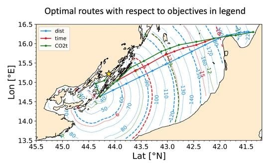
1. Introduction
Regulatory action on maritime emissions has gained momentum during the last couple of years.
In April 2018, the International Maritime Organization (IMO) adopted an “Initial Strategy” to halve global shipping emissions by mid-century, and more specifically reduce carbon intensity by 40% by 2030, taking 2008 as a baseline year [1]. The strategy, considered a milestone by IMO, was structured into levels of ambition and candidate measures. The measures included short, medium, and long-term time horizons. While in the long term most ships should adopt zero-carbon fuels, in the medium term this should be enabled by both technical developments and market based measures (MBM). For the short term, IMO proposed both design and operational measures. The latter includes energy efficiency gains via a Ship Energy Efficiency Management Plan (SEEMP). It considers cost-efficient measures such as speed optimization and speed reduction, and the quantification of savings via the Energy Efficiency Operational Indicator (EEOI) [2]. Very recently, IMO has approved new mandatory measures for reduction of Greenhouse Gases (GHGs) in the short term, including a rating scheme based on carbon intensity indicators (CII) and a SEEMP enhancement for making a CII reduction plan mandatory [3].
The pillars of the European Union (EU)’s vision are the “Climate Action” and the European Green Deal1. The final goal is to decarbonize all sectors of the European economy by 2050. In particular, shipping was already in the sights of the EU in 2015, as a Regulation on Monitoring, Reporting, and Verification (MRV) of CO emissions [4] entered into force for ships above 5000 Gross Tonnes (GT) calling at ports of the European Economic Area (EEA). This led to the first-ever publication of a ship-distinctive database of emissions (2019). For ferries, an assessment of these data was done in [5]. The Regulation entered an amendment procedure that, following a proposal approved by the European Parliament (EP) in September 20202, will probably make its ambition bigger. Indeed, the EP approved reporting of all GHGs (not just CO), inclusion of ship emissions into the European Emission Trading Scheme (EU-ETS, which is a form of MBM), and a linear reduction of CO emissions per transport work of 40% by 2030 with respect to 2018 [6].
Therefore, energy efficiency or carbon intensity is a possible point of convergence between IMO and EU regulations. To this end, it is important to objectively quantify the potential of efficiency measures. This requires, as a minimum, to agree on metrics and baselines. Indeed, besides EEOI, several other CIIs have been proposed and used so far. They are all expressed as ratios of CO emissions to some proxy of vessel’s transport work, as reported in Table 1.
Some peer-reviewed works document EEOI estimation for ocean routes through simulated optimization of the voyages. In [9], a quantity closely related to EEOI is computed starting from speed loss in waves and is compared to recorded operational data from noon reports of two oil tankers. In [10] a back propagation neural network is used for assessing that, in ice-covered waters in the Arctic, EEOI mainly depends on ship speed and ice concentration. In [11], least-time routes in the Atlantic considering both ocean currents and waves were computed, assessing both the regional and seasonal dependence of the EEOI savings with respect to least-distance routes. Finally, Reference [12] addresses the role of ship speed on cost and energy efficiency, while Reference [13] reviews several other works dealing with ship fuel efficiency of routes in relation to marine weather conditions.
In [11], significant ship diversions were computed for the optimal routes because of their long duration (from days up to more than a week) and the large extent of the spatial domain in direction normal to the least-distance paths (thousands of nautical miles, nmi). One may wonder if path optimization may play a role even on shorter temporal ranges and spatially stretched domains. Also, while weather conditions in the ocean may lead to quite rough sea states (a maximum significant wave heights in excess of 18 m was recorded3), both average and extreme conditions in other seas may be far less challenging for navigation.
The Adriatic Sea, with a maximum of about 3 m [14] and a maximum width of just about 100 nmi in direction normal to its elongation axis, is an interesting candidate domain in contrast to the open ocean for testing the role of ship route optimization. The Adriatic Sea is routinely crossed by several ferry lanes joining ports in Italy with ports in Croatia, Montenegro, and Albania. Also, according to the MRV dataset of 2018, despite the fact that the number of Ro-Pax ships (transporting both vehicles and passengers) was only about 3% of all ships reporting calls in the EEA, the quota of their CO emissions was an over-proportional 10% [5].
From these considerations, a few questions arise: Can path optimization play a role even in the Adriatic? What CO savings are potentially attainable? How much can ferries’ carbon intensity be decreased? What is the relative role of waves and currents?
To address these questions, we have upgraded the VISIR (discoVerIng Safe and effIcient Routes) ship routing model from [11,15] to a “VISIR-2” version. It includes several technical innovations for enabling the present and other future investigations. Here, we just focus on a preview of VISIR-2 potential, before a dedicated paper will accompany the release of its source code. Therefore, this paper’s Section 2 reviews such VISIR innovations, before the results are presented in Section 3. The conclusions are then drawn in Section 4.
2. Materials and Methods
The results in this work were obtained by means of numerical simulations based on the VISIR ship routing model4. In particular, a new, Python-coded version of the model released through [11,15] was designed, developed, and deployed to the region of interest. The VISIR-2 model is not simply a recoding of its Matlab ancestor VISIR-1. Indeed VISIR-2 presents a number of architectural innovations and new features. VISIR-1, whose path planning component underwent a severe validation process (also through comparison to a PDE-based model [16]), was used as a benchmark for the VISIR-2 results. Here we just list some of the technical novelties of VISIR-2:
- Least-CO routes. VISIR can compute optimal routes by suggesting a spatial diversion which leads to avoidance of rough sea and related ship speed loss. Besides least-distance and least-time routes, we added a capacity to compute routes of least-total-CO emissions. This required a further generalisation of the time-dependent Dijkstra’s algorithm which is at the core of VISIR [15]. To this end, it is not enough to feed the routine with edge weights corresponding to the CO emissions along each edge. Indeed, the time for sailing through each edge (“edge delay”) should still be provided, in order to evaluate the position of the vessel and the environmental conditions encountered and the duration of the route. The related pseudocode will be published elsewhere;
- Visualization. Mapping of the routes was improved by including the fronts of the locations reachable within a given time since departure (isochrones) and the environmental fields were sliced among isochrones. The latter were compared with lines of equal distance from route origin (or: “isometres”) and lines of equal amount of CO emissions (or: “isopones”), cf. Table 2. The name isopone is related to energy consumption (the greek word means “equal effort”), which is proportional to CO emissions;
- Vessel performance modeling. In addition to the VISIR-1 model based on a dynamic balance at the propeller and parametrisation of calm water and wave-added resistance [15], an alternative vessel model was introduced in VISIR-2. It made use of the outcome of a ship simulator, from which the performance and emissions of a ferry were estimated in various sea conditions. This is described in more detail in Section 2.1. The Speed Through Water (STW) resulting from this approach can then be combined with the sea surface currents for computing the Speed Over Ground (SOG), along the way already demonstrated in [11].
2.1. Ship Simulator
The University of Zadar hosts at its premises a coupled command-bridge engine-room simulator. For this project, a data package for simulating a specific ferry was acquired.
The simulator consisted of the “Wärtsilä-Transas Marine NTPro 5000 Navigation Simulator” command-bridge simulator with a realistic console coupled to the “Wärtsilä ERS-LCHS 5000 TechSim” engine-room and cargo-handling simulator.
The vessel type considered for this work was a Ro-Pax ferry with a twin, four-stroke engine (MAN Diesel 32/40 Twin Medium Speed)5 with controllable pitch propeller (cpp). The vessel also included cpp bow thrusters (hydraulic system not modelled) with a power of 1000 kW and two fin stabilizers which may or may not be active. Trim was not adjustable for this vessel. Other vessel characteristics are provided in Table 3.
The simulator was operated with the following configuration: no sea currents (they can be added later to the ship kinematics as done in [11]), no swell, and wind-waves according to the relation found in [14]. This implies collinear wind and waves, as also assumed in [9], and a quadratic dependence between wave height and wind intensity—for more general models including also fetch, see e.g., [19]. The relative wind-to-ship heading true direction was variable in the range 0 (head seas) to 180 (following seas), while the fractional engine load could vary in the 70 to 100% range.
The recorded output variables were: STW, power delivered at the propeller shaft (P), and specific fuel oil consumption (SFOC). The latter two resulted from averaging of the values for the twin main engines. For each simulator setup (i.e., values of wind magnitude and direction plus engine load), a time dependent signal was recorded for about 25 min long, its initial transient dynamics (about 2 min) were pruned, and the remaining signal (which was quite constant) averaged. Stabilizer fins of the ferry hull were not active.
The 3-dimensional (3D) space of the input setup (wind magnitude and direction and engine load) was sampled after simpler 1D tests revealed the relevant region useful for inferring the vessel dynamics. The multi-dimensional dependence of each output variable (STW, P, SFOC) was fitted by means of a cascade of 1D least-square fits, each using elementary functions only (polynomial, trigonometric, or exponential functions). More details on the fitting procedure will be published elsewhere. The final fit function was evaluated vs. the observed data (i.e., the simulator data) in terms of standard statistical metrics (bias, rmse, correlation coefficient).
Finally, the CO emission rate (tons CO emitted per hour) was computed as:
with the conversion factor g/g accounting for a marine diesel oil fuel [2]. Emissions from the auxiliary engine were not considered, as during the simulation each was loaded at only about one quarter of the power reported in Table 3. The total CO emission were obtained by integrating the rate of Equation (1) along the ship path. A generic CII was computed as the ratio of total CO emissions to some representation of transport work :
where L was the length of the path and a measure of the cargo carried by the vessel. Depending on the actual intensity indicator, may take different functional forms, as reported in Table 1. However, all the selected indicators depend on L in a multiplicative way.
2.2. Environmental Fields
VISIR-2 makes use of both static and dynamic environmental fields as in the following.
- Bathymetry. The EMODnet bathymetric database6 was used for checking that navigation does not occur in shallow waters. Given its high spatial resolution (1/16 arc minute or about 120 m in the meridional direction), the bathymetry was also used to derive a pseudo-shoreline. It went this way: An under keel clearance map UKC = was computed from the bathymetry map (z) and the vessel draught (T). The contour line at UKC = 0 defined a pseudo-shoreline, which was then used for pruning graph edges crossing it;
- Waves. Sea state analysis products were obtained through CMEMS (Copernicus-Marine Environment Monitoring Service)7 from the operational analysis and forecast system by HCMR (Hellenic Centre for Marine Research) for the Mediterranean Sea, based on wave model WAM Cycle 4.6.2. The dataset name was MEDSEA_ANALYSIS_ FORECAST_WAV_006_017. Significant wave height and direction fields were used. They had hourly time resolution and 1/24 degree (2.5 nmi8 in the meridional direction) horizontal resolution;
- Currents. Sea circulation analysis products were obtained through CMEMS from the operational analysis and forecast system by CMCC (Euro-Mediterranean Center on Climate Change) for the Mediterranean Sea, based on NEMO v3.6 coupled to wave model WW3 and making use of a 3DVAR data assimilation scheme. The dataset name was MEDSEA_ANALYSIS_FORECAST_PHY_006_013. Surface level meridional and zonal currents were used. They had hourly time resolution and 1/24 degree horizontal resolution.
3. Results
This section presents an essay of computational results from VISIR-2 obtained according to the methodology of Section 2. The results from the bridge-engine coupled simulator and their analysis are given in Section 3.1; the isolines relative to the various optimization objectives are discussed in Section 3.2; a visualization of the bundles of routes in Section 3.3; and the analysis of carbon intensity savings resulting from CO-optimal routes is provided in Section 3.4.
3.1. Vessel Performance
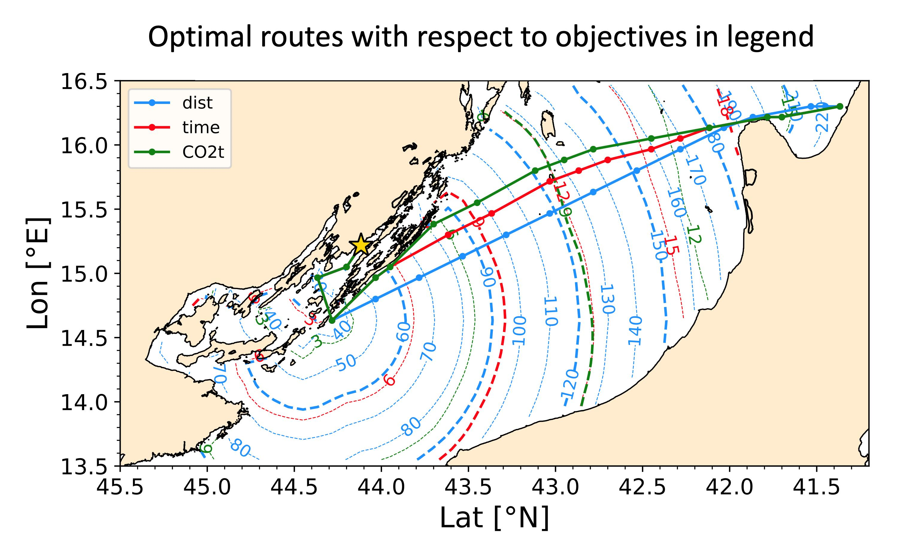
Figure 1 displays a subset of the multidimensional information collected at the ship simulator and processed as in Section 2.1, together with the fitted trends for identifying the vessel model parameters.
The ferry speed loss as a function of significant wave height can be well fitted by a logistic function, with a decay length which turns to be adequately captured by the chosen sampling of the simulator response, Figure 1a. For a given , the spacing between STW values relative to contiguous values is, in the range explored, nearly constant. Also, this spacing decreases from 1.5 to 1.2 kts as increases from 0 to 4 m. A qualitatively similar trend was also found in ([11,15] [Figure 4]) and should be due to the decreasing influence of calm water with respect to the wave-added resistance as increases or decreases. However, vessel resistance as a simulator output is unfortunately not available to check this interpretation.
The dependence of STW on the true angle of attack of wind, , can be fitted by a hyperbolic tangent, Figure 1b. Maximum speed loss occurs for head seas, with a sharp reduction from head to following winds occurring at . This is possibly related to the asymmetry of the vessel’s superboard. Several works compared the computed to the observed speed loss in waves, focussing on larger vessels and mainly on head seas [20,21]. The impact of oblique seas on speed loss is less documented but a promising computational approach was presented in [22].
The CO emission rate is computed from Equation (1) and displayed in Figure 1c,d. For a given sea state (angle of attack of wind and significant wave height), it increases threefold as raises from 70 to 100%. However, for a given angle of attack and engine load, dCO2/dt still varies with by more than 10% at the lowest load (Figure 1c). For a given load and significant wave height, it also changes with the angle of attack in an appreciable way, especially at large , where it reduces by about 10% as one goes from head to following sea (Figure 1d).
In order to understand these results, it should first be recalled that, as a combinator mode is used for this vessel’s propulsion system, engine rotation rate and fractional engine load are nearly proportional. Their relation is found to be given by rpm. As seen from Figure 1a,c, accounts for most of the variability of both STW and emission rate. The residual variability is ascribed to the running conditions of the propeller. As they–because of rougher or more head seas–become heavier, power delivered at the propeller shaft increases, while SFOC decreases (Figure 1e,f). Power is not shown here, but can be obtained from Equation (1) and the data in Figure 1c–f.
Finally, we note that fitting of the directional dependence of both STW and dCO/dt might suffer from undersampling of the simulator response. However, the overall quality of the multidimensional fits with respect to the original datapoints from the ship simulator was assessed through standard metrics as reported in Table 4 and resulted to be quite satisfactory.
3.2. Isolines
In Figure 2a hypothetical ferry connection between Zadar (Croatia) and Barletta (Italy) is considered. The route optimization was performed on a graph with a grid spacing = 1/12. This implies a linear resolution of 5 nmi in the meridional direction and, for the considered domain, about 3.6 nmi in the zonal direction. Furthermore, graph nodes were linked by up to four-hop edges. Such a level of connectivity ( = 4) implies a directional resolution of 14. In the future, it will be possible to assess the optimal trade-off between horizontal and angular resolution, along the method of [16].
In Figure 2, all three types of optimal routes of are displayed: with respect to distance, duration, and CO emissions. In addition, for each optimization type, corresponding isolines as from Table 2, are shown. It can be noted that each isoline is locally normal to its related optimal route. This property of normality follows from optimality: the isolines are fronts of the 2D field of the optimization objective. In a partial differential equation approach [23], the isolines would correspond to the level set functions. In Figure 2, small deviations from normality are due to the graph resolution, affecting both the land-sea mask and inter-waypoint distance.
However, the presence of isochrones should not mislead the reader: in VISIR, path optimization is still based on Dijkstra’s algorithm. The various isolines join all locations reachable from the origin with a given expenditure of the objective function (distance, time, or CO). A remarkable property of Dijkstra’s algorithm is that such function values are assigned at the same computational cost of assigning the value of the objective function at a single location on the same front [24].
In Figure 2 it is seen that both the time- and CO-optimal routes divert inshore towards Croatia. As already noted in [15] this is Snell’s refraction in action due to the coastal environmental conditions favouring a slower increase of the objective functions. This understanding in terms of route refraction is complemented by the isolines, which bulge along gradients of the 2D field of the objective function. This is visible for the isopone at 9 t CO, bulging towards the island of Vis (Croatia). Also, a few recessions of the isolines are noted in correspondence of islands: a navigational obstruction makes its downwind side reachable only upon a diversion, which increases the length of the trajectory and, consequently, both the sailing time needed to reach it and related emissions.
The fact that CO- and time-optimal routes have similar spatial features follows from the weak dependence of the CO rate on , as seen in Figure 1d. Indeed, per Equation (1), this implies that, for the present vessel model, the CO emissions along each edge are roughly proportional to the time needed for sailing across them.
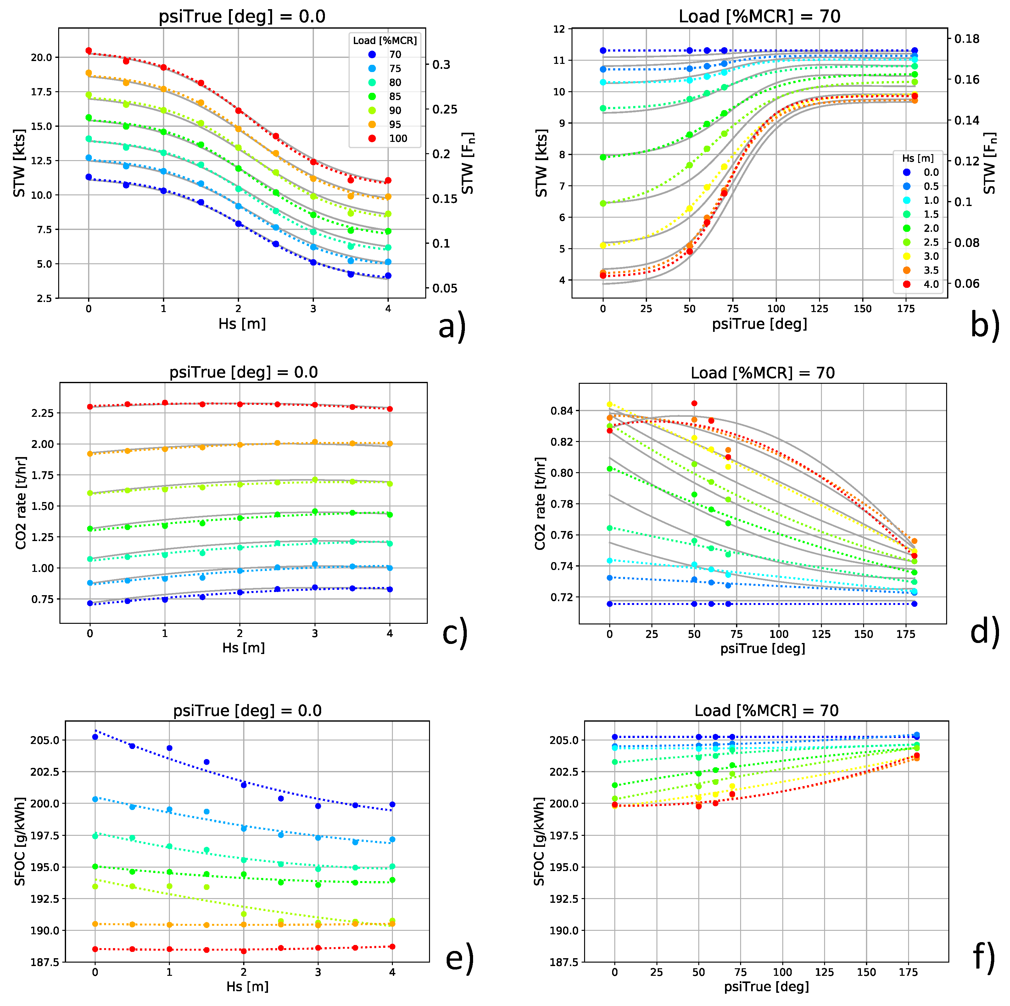
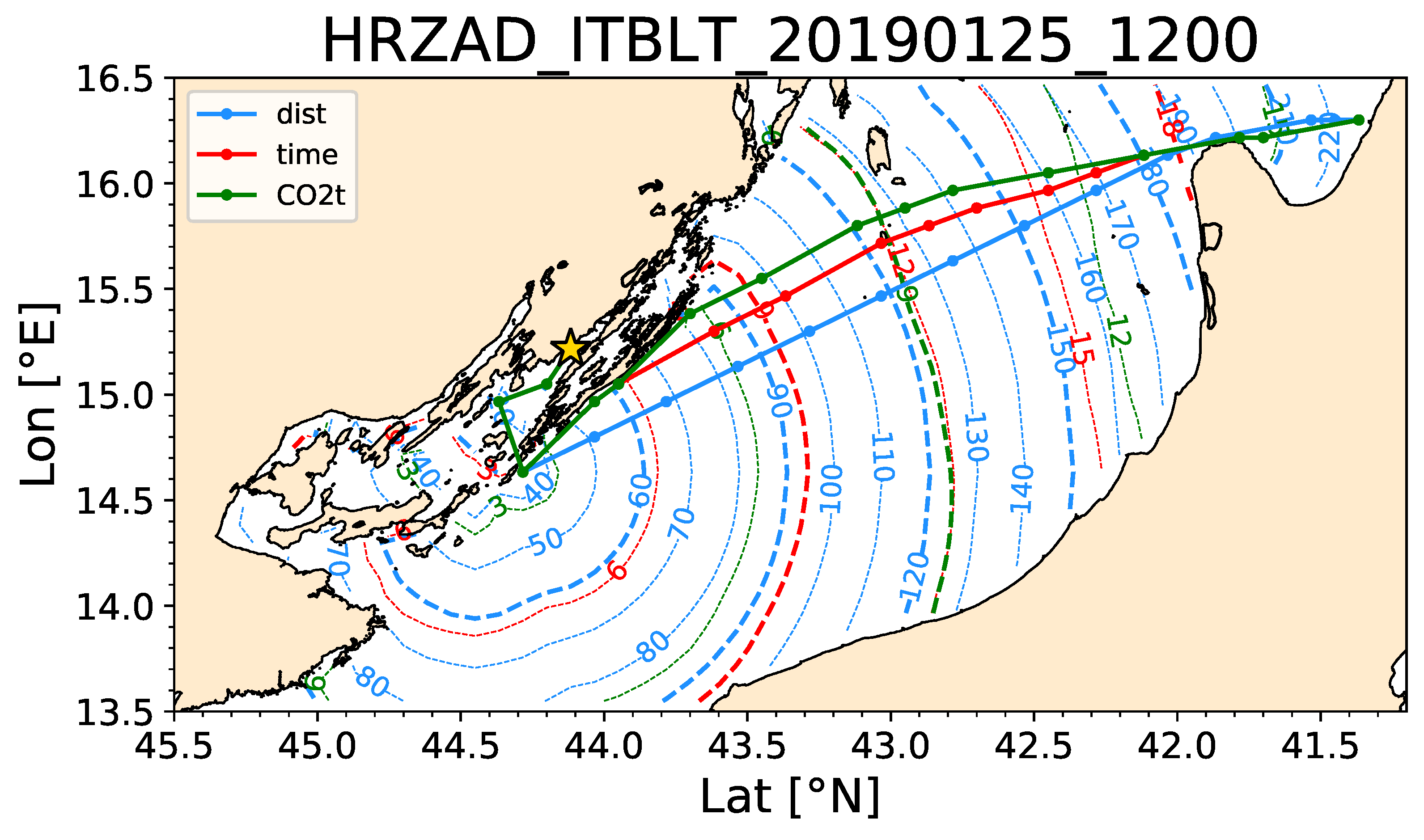
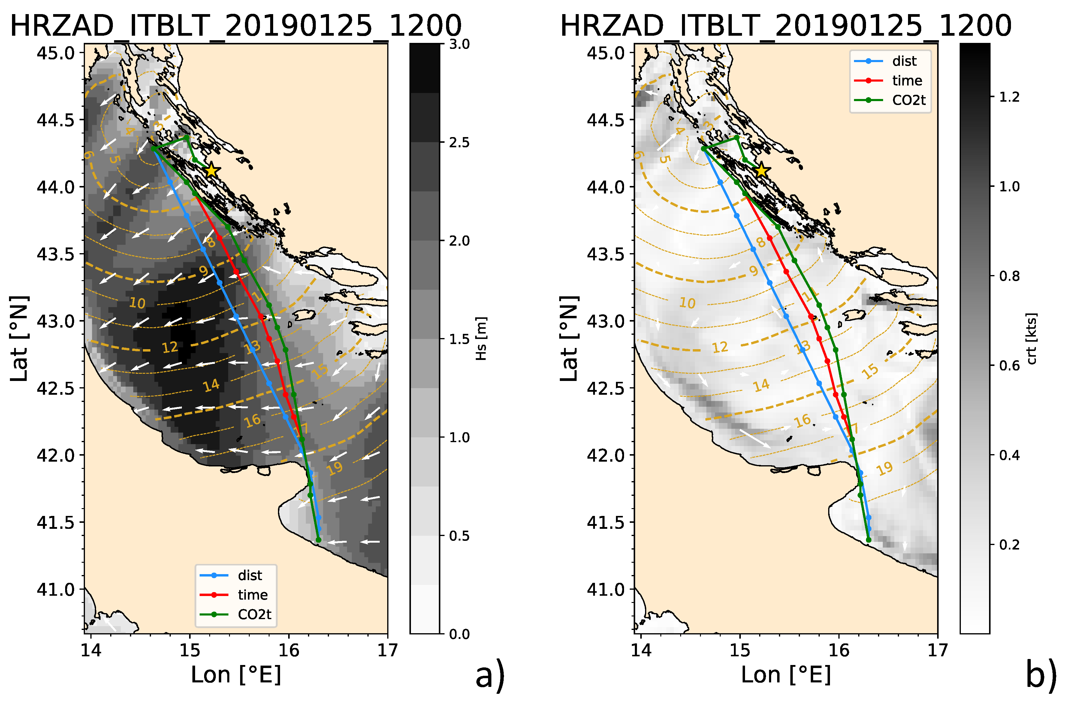
Visualising also the environmental conditions, Figure 3 shows that, between 9 and 15 h since departure, a rough sea develops in the central Adriatic. The least-distance route crosses it. Instead, both the time- and CO optimal routes avoid it by diverting to port, in order to experience smaller . For this simulation, the most prominent feature of sea surface circulation is the (southbound) Western Adriatic Coastal Current, next to the Italian shore [25], and some local flow strengthening at the southern side of the island of Hvar, Croatia. Other currents in the northern and southern part of the domain are too far to influence the optimization of these routes. It should be noted that the chosen graph resolution still allows to compute a passage south of the island of Premuda, a maritime gateway next to the port of Zadar.
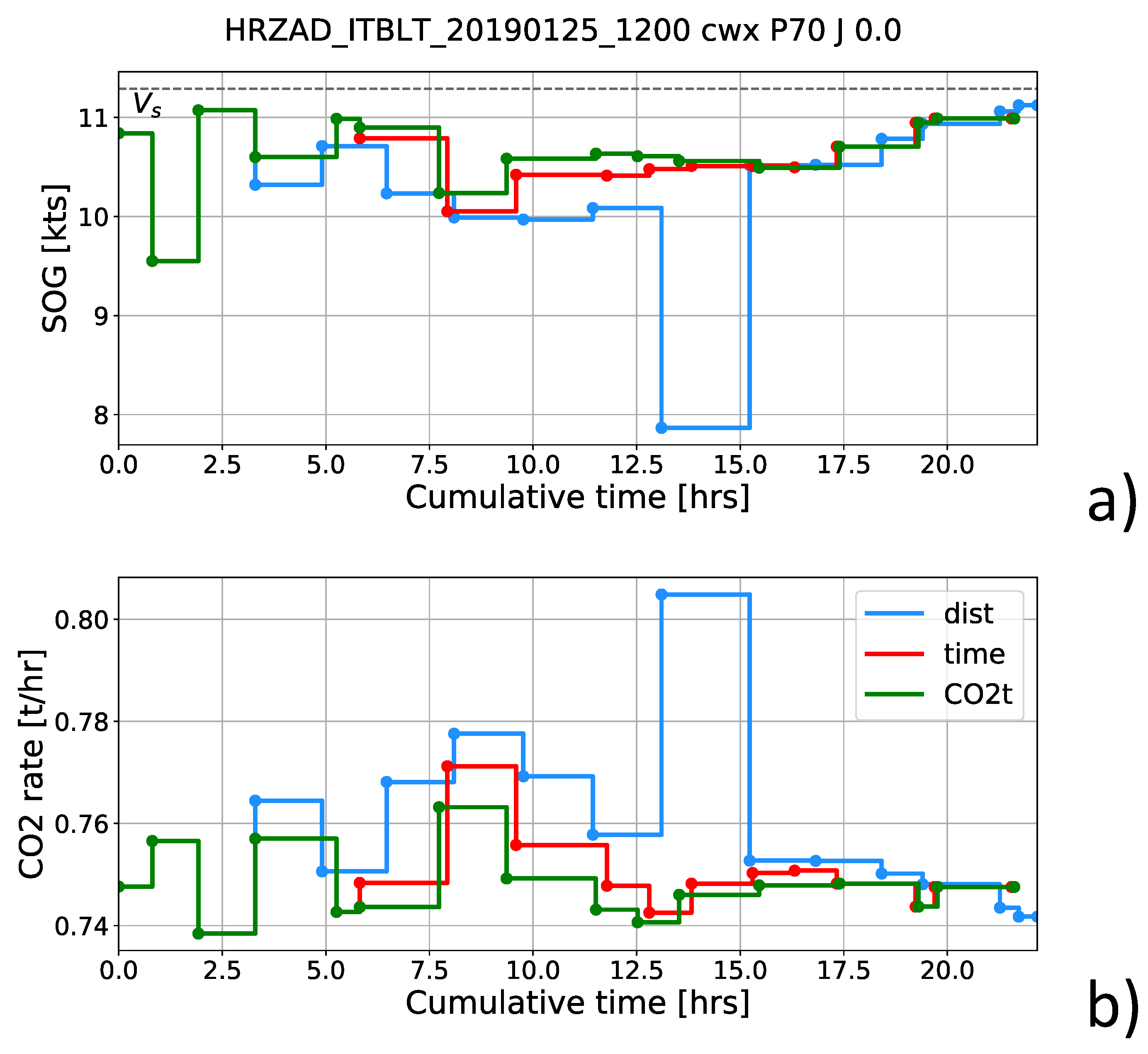
The optimality of the routes is also investigated by the linecharts of Figure 4. They display along-route information vs. cumulative time since departure. Thanks to the diversion towards the Kornati islands (Croatia), optimal routes SOG are generally higher (Figure 4a) and the CO emission rates lower (Figure 4b) than along the least-distance route. This is especially true at times 13–15 h since departure, as the least-distance route crosses the peak of rough sea in central Adriatic while the optimal routes have advanced more towards destination and sail more inshore, towards Vis. As safety constraints for vessel intact stability [15] have not yet been implemented into VISIR-2, the time-optimal route always had a shorter duration, and the CO-optimal route always had a lower total CO emission than the least-distance route (Table 5).
3.3. Spatial Diversions
Case study results given in Section 3.2 are instrumental in documenting a methodology. How representative of the potential of the Adriatic Sea for Ro-Pax route optimization are they? How large can spatial diversions be as the environmental conditions are varied? While systematic investigations on different routes and dates will be performed through an operational tool to be developed in the frame of the GUTTA project9, some preliminary results are reported in this subsection.
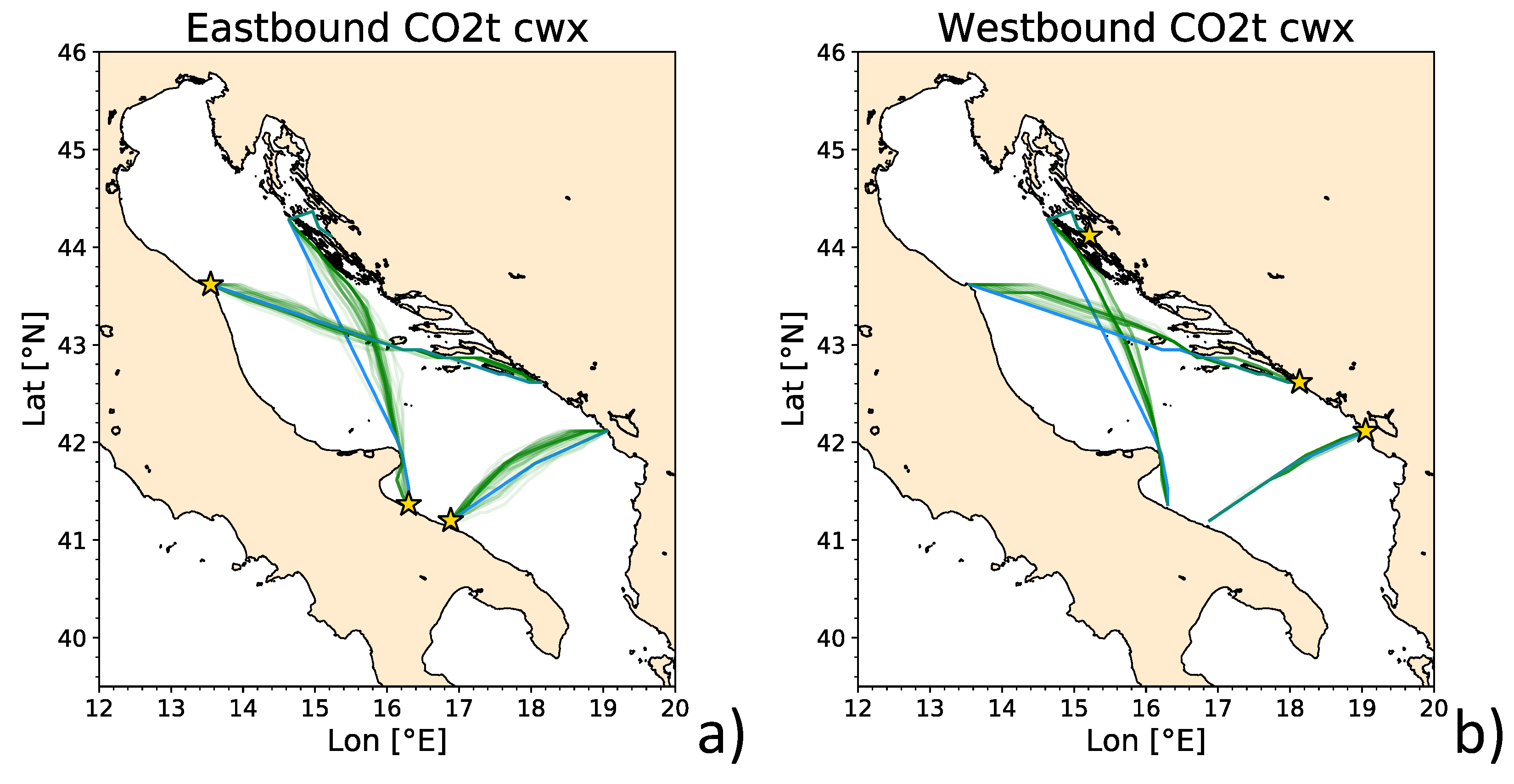
A set of CO2-optimal routes are displayed for three different crossings of the Adriatic, for both Eastbound (Figure 5a) and Westbound passages (Figure 5b). Some of these cross border links are presently just hypothetical and not yet served by any ferry connection. The seaports involved are listed in Table 6.
In order to compute the results in Figure 5, one given departure date (25 January 2019), eight departure times per day (at 00Z10, 03Z, etc.), seven fractional engine loads between 70 and 100% were used for each of the three oriented crossings of the Adriatic Sea. This resulted in 336 optimizations with respect to each of the three objectives (distance, time, CO).
On departure date, the general sea conditions were dominated by North-Easterly winds. For each crossing, bundles with appreciable diversions from the least-distance route are seen. Generally, diversions on either side of the least-distance route are computed. For both the Zadar-Barletta and way back, mainly inshore diversions towards the Dalmatian coast result. The optimal routes of the Ancona-Dubrovnik crossings may sail on either side of Mljet and, for the way back, also Vis islands, which is an example of route topological change induced by the optimization. Spatial diversions for this and the other crossings are mainly driven by the sea state (leading to approach more favourable sea states inshore) and by the directional dependence of the speed loss in waves, cf. Figure 1b. For instance, the Bar-Bari route is in most case fairly aligned with the wind-wave course, leading to minimum speed loss in absence of diversions. Instead, the Bari-Bar optimal route can divert significantly either North or South. This is primarily due to wave avoidance, but also in part to the presence of the Southern Adriatic gyre [25]. Indeed, the optimal routes can occasionally profit of superposition of STW with one of its meanders (not shown). A similar mechanism was seen in action on a much larger space and time scale in the Atlantic Ocean, for routes being advected or avoiding the Gulf Stream, depending on their general course [11].
The actual spatial diversions computed for these routes depend on the details of the vessel response functions given in Figure 1. For instance, a wind-wave relationship different from what used and documented in Section 2.1 may lead to different optimal routes. To what extent this choice impacts the results is left for future investigations.
3.4. Carbon Intensity Savings
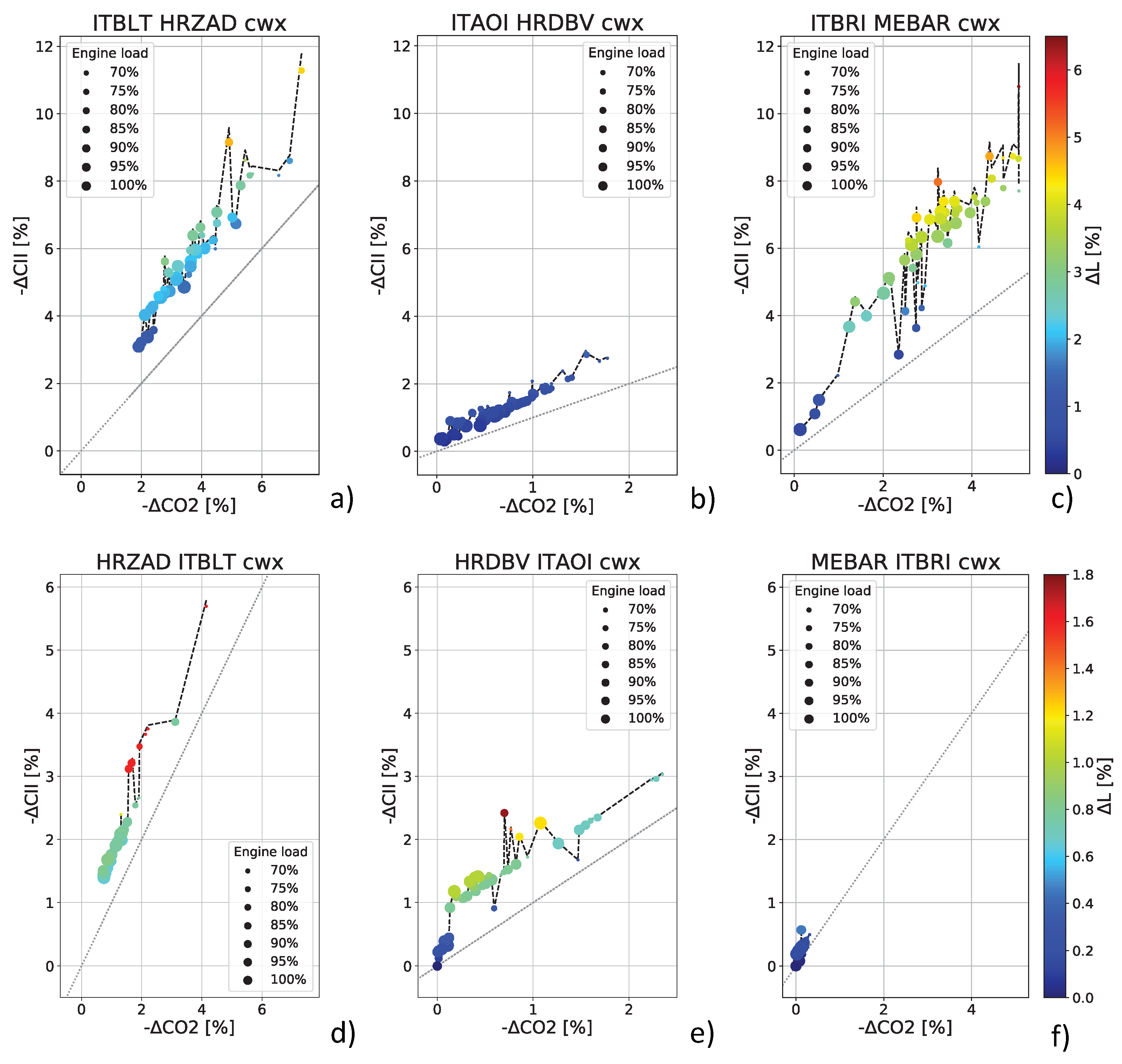
The final purpose of this work was to assess the potential of route optimization in the Adriatic Sea with respect to carbon intensity savings (cf. Section 1). The generic CII of Equation (2) was used for this purpose. Its changes with respect to the least-distance routes are displayed in Figure 6 vs. corresponding changes in total CO emissions. The relative savings are limited by a value which, besides the CO saving, also includes the relative lengthening of the sailed path:
where indicates the relative change of the quantity with respect to the least-distance route. Equation (3) can be derived from Equation (2) using the theory of error propagation [26] and the fact that, comparing these two routes, both CII and CO decrease as the path length L increases.
CO savings up to 7% and CII savings up to 11% are computed on the Barletta-Zadar, while for the other crossings the savings are smaller, down to the Bar-Bari crossings where, for the chosen date of simulation, they vanish.
The data in Figure 6 show that the CII relative savings are nearly always given by the value predicted by Equation (2). In most cases, even the equality holds, meaning the relative path lengthening adds up with the relative CO savings to produce the relative CII savings.
If coastal diversions and obstructions were negligible, would just increase with the curvature of the optimal route with respect to the least-distance one. This is apparent for instance in the case of two Italy-Montenegro crossings.
No clear relationship between CII savings and fractional engine load is seen. This should be investigated deeper for a larger set of routes, also in relation to ship engine power limitation (EPL), a proposed measure for emission reduction discussed also at the latest IMO MEPC meeting [3].
It should be emphasized that, for given environmental conditions, even the specific graph (grid resolution and connectivity, cf. [16]) and vessel response function (Section 3.1) are expected to affect the actual magnitude of the CII savings. While being beyond the scope of this paper, it is in principle possible to provide a confidence interval for the CII savings by keeping into account this source of error.
4. Conclusions
This work addressed carbon intensity reduction through voyage optimization in short sea shipping.
The VISIR ship routing model was upgraded to its version 2 in order to use a ferry response function fitted on data collected through a command-bridge engine-room coupled simulator. This way, the vessel model was actually less general than in VISIR-1, but allowed for a more accurate estimation of ship speed loss in waves, as well as for an explicit assessment of CO emission rates. The simulator enabled extracting the ferry response even as a function of the angle of attack of wind and for various fractional engine loads.
Furthermore, VISIR-2 includes the capacity to compute least-CO routes, in addition to least-distance and least-time routes. The effect of optimization on carbon intensity indicators was quantified. Using CMEMS ocean analysis products related to waves and sea currents, several case studies were computed for crossings of the Adriatic Sea. The visualization of the outputs of VISIR was enhanced by the computation of the isolines corresponding to the various optimization objectives.
In presence of rough seas, the CO-optimal routes were found to significantly differ from least-distance routes. Related CO savings depend on the actual crossing considered, with a top value of 7%. Correspondingly, the CII savings reached up to 11%. Winter navigation conditions with a specific wind pattern were selected for our case study. The statistical significance of this figure could not yet be assessed, as systematic investigations in presence of different other meteo-oceanographic conditions are still to come. However, savings of this size are encouraging, as it represents a significant amount of the carbon intensity curbing target by both IMO and EU.
Furthermore, such savings are demonstrated for a Ro-Pax vessel. This is remarkable, as CO emissions from this ship type are over-proportional with respect to their abundance in the fraction of the EEA fleet due to report per EU-MRV [5]. Also, present-day energy efficiency of ferries may not always be competitive with land-based alternatives, as pointed out in [7]. A rating scheme for CII or even a “carbon intensity code” might be adopted for several ship types in the near future by IMO [3] and CO emissions from shipping might be subjected to MBMs in Europe. Thus, this work supports the thesis that voyage optimization, in combination with EPL, could be a viable operational measure for short-sea shipping to meet short-term targets for both absolute emission and carbon intensity reduction.
Concerning the spatial features of the computed optimal routes, bundles of appreciable spatial diversions were retrieved, with a hint to a not negligible role played not only by waves but also by surface sea currents. Such diversions occur on a much shorter space and time scale than in the ocean [11], posing the question of ship manoeuvrability. While it needs to be assessed in cooperation with the relevant stakeholders, the present results demonstrate on the scale of short-sea shipping an effect that had previously been known at ocean scale only. This is ascribed to the simultaneous availability of both high resolution ocean forecasting products and a routing model (VISIR) able to work even in coastal and archipelagic domains, such as coastal Croatia.
The sources of uncertainty for our results are: the ocean analysis products, the spatial and angular discretization (in the graph), and the vessel response model.
The quality of the CMEMS forecasting and analysis products is routinely monitored with respect to multiple sources of observations and published in quality information documents (QUID). The information in the QUIDs is resolved at sub-regional scale and updated on quarterly basis. For the wave product used, the significant wave height is accurately predicted, with best performance in winter and in open seas. For the sea currents product, there are fewer direct measurements and the assessment for the Adriatic region is less satisfactory than the Mediterranean Sea average.
The path optimization algorithm did not make use of any free parameters: it was intrinsically exact (based on Dijkstra’s algorithm) and had previously been validated in multiple ways. However, in future both the linear and angular resolution of the graph used for the VISIR computations could be tuned for even more accurate estimations of the CO emissions and emission intensity metrics.
Alternative wind-wave relationships could be used, for instance additionally considering swell and crossed seas, which would result in a potentially different vessel dynamical response. Even for the present wind-wave parametrization, the simulator’s vessel response could be sampled more densely, which may lead to choosing more proper fitting functions, especially for its angular dependence. Furthermore, no constraints on vessel intact stability [15] have been coded into VISIR-2 yet. Once included, they may lead to specific spatial diversions affecting both the CO and the CII savings.
We aim to have at least some of these additional investigations and improvements ready for the first public release of the VISIR-2 source code.
Author Contributions
Conceptualization, G.M.; methodology, G.M.; software, L.C. and C.P.M.; validation, G.M. and L.C.; formal analysis, G.M., L.C.; investigation, L.C., J.O.; resources, G.C., J.O.; data curation: L.C.; writing–original draft preparation, G.M.; writing–review and editing, G.M., C.P.M., J.O., G.C.; visualization, L.C.; supervision, G.M.; project administration, G.M.; funding acquisition, G.M., G.C. All authors have read and agreed to the published version of the manuscript.
Funding
This research was funded by the European Regional Development Fund through the Italy-Croatia Interreg programme, project GUTTA, grant number 10043587.
Institutional Review Board Statement
Not applicable.
Informed Consent Statement
Not applicable.
Data Availability Statement
The source files of the figures are available upon request.
Conflicts of Interest
The authors declare no conflict of interest. The funders had no role in the design of the study; in the collection, analyses, or interpretation of data; in the writing of the manuscript, or in the decision to publish the results.
References
- IMO. MEPC.304(72) Initial IMO Strategy on Reduction of GHG Emissions from Ships; Technical Report Annex 11; International Maritime Organization: London, UK, 2018. [Google Scholar]
- IMO. MEPC.1/Circ.684 Guidelines for Voluntary Use of the Ship Energy Efficiency Operational Indicator (EEOI); Technical Report; International Maritime Organization: London, UK, 2009. [Google Scholar]
- IMO. MEPC 75/WP1/Rev.1 Draft Report Of The Marine Environment Protection Committee On Its Seventy-Fifth Session; Technical Report; International Maritime Organization: London, UK, 2020. [Google Scholar]
- EU. Regulation 2015/757 of 29 April 2015 on the Monitoring, Reporting and Verification of Carbon Dioxide Emissions from Maritime Transport, and Amending Directive 2009/16/EC; Technical Report; European Parliament and the Council: Brussels, Belgium, 2015. [Google Scholar]
- Mannarini, G.; Carelli, L.; Salhi, A. EU-MRV: An analysis of 2018’s Ro-Pax CO2 data. In Proceedings of the 21st IEEE International Conference on Mobile Data Management (MDM), Versailles, France, 30 June–3 July 2020; pp. 287–292. [Google Scholar] [CrossRef]
- EP. Amendments Adopted by the European Parliament on 16 September 2020 on the Proposal for a Regulation of the European Parliament and of the Council Amending Regulation (EU) 2015/757 in Order to Take Appropriate Account of the Global Data Collection System for Ship Fuel Oil Consumption Data (COM(2019)0038–C8-0043/2019—2019/0017(COD)); Technical Report; European Parliament: Brussels, Belgium, 2020. [Google Scholar]
- Zis, T.P.; Psaraftis, H.N.; Tillig, F.; Ringsberg, J.W. Decarbonizing maritime transport: A Ro-Pax case study. Res. Transp. Bus. Manag. 2020, 37, 100565. [Google Scholar] [CrossRef]
- Panagakos, G.; Pessôa, T.d.S.; Dessypris, N.; Barfod, M.B.; Psaraftis, H.N. Monitoring the carbon footprint of dry bulk shipping in the EU: An early assessment of the MRV regulation. Sustainability 2019, 11, 5133. [Google Scholar] [CrossRef] [Green Version]
- Lu, R.; Turan, O.; Boulougouris, E.; Banks, C.; Incecik, A. A semi-empirical ship operational performance prediction model for voyage optimization towards energy efficient shipping. Ocean Eng. 2015, 110, 18–28. [Google Scholar] [CrossRef] [Green Version]
- Zhang, C.; Zhang, D.; Zhang, M.; Mao, W. Data-driven ship energy efficiency analysis and optimization model for route planning in ice-covered Arctic waters. Ocean Eng. 2019, 186, 106071. [Google Scholar] [CrossRef]
- Mannarini, G.; Carelli, L. VISIR-1.b: Ocean surface gravity waves and currents for energy-efficient navigation. Geosci. Model Dev. 2019, 12, 3449–3480. [Google Scholar] [CrossRef] [Green Version]
- Psaraftis, H.N.; Kontovas, C.A. Speed models for energy-efficient maritime transportation: A taxonomy and survey. Transp. Res. Part C Emerg. Technol. 2013, 26, 331–351. [Google Scholar] [CrossRef]
- Zis, T.P.; Psaraftis, H.N.; Ding, L. Ship weather routing: A taxonomy and survey. Ocean Eng. 2020, 213, 107697. [Google Scholar] [CrossRef]
- Farkas, A.; Parunov, J.; Katalinić, M. Wave statistics for the middle Adriatic Sea. Pomor. Zb. 2016, 52, 33–47. [Google Scholar] [CrossRef]
- Mannarini, G.; Pinardi, N.; Coppini, G.; Oddo, P.; Iafrati, A. VISIR-I: Small vessels – least-time nautical routes using wave forecasts. Geosci. Model Dev. 2016, 9, 1597–1625. [Google Scholar] [CrossRef] [Green Version]
- Mannarini, G.; Subramani, D.; Lermusiaux, P.; Pinardi, N. Graph-Search and Differential Equations for Time-Optimal Vessel Route Planning in Dynamic Ocean Waves. IEEE Trans. Intell. Transp. Syst. 2019, 21, 3581–3593. [Google Scholar] [CrossRef] [Green Version]
- Hagiwara, H. Weather Routing of (Sail-Assisted) Motor Vessels. Ph.D. Thesis, Technische Universiteit Delft, Delft, The Netherlands, 1989. [Google Scholar]
- Klompstra, M.B.; Olsder, G.J.; van Brunschot, P.K.G.M. The isopone method in optimal control. Dyn. Control 1992, 2, 281–301. [Google Scholar] [CrossRef]
- Bitner-Gregerse, E.M.; Guedes Soares, C.; Vantorre, M. Adverse weather conditions for ship manoeuvrability. Transp. Res. Procedia 2016, 14, 1631–1640. [Google Scholar] [CrossRef] [Green Version]
- Vitali, N.; Prpić-Oršić, J.; Guedes Soares, C. Coupling voyage and weather data to estimate speed loss of container ships in realistic conditions. Ocean Eng. 2020, 210, 106758. [Google Scholar] [CrossRef]
- Lang, X.; Mao, W. A semi-empirical model for ship speed loss prediction at head sea and its validation by full-scale measurements. Ocean Eng. 2020, 209, 107494. [Google Scholar] [CrossRef]
- Tsujimoto, M.; Kuroda, M.; Shibata, K.; Sogihara, N.; Takagi, K. On a calculation of decrease of ship speed in actual seas. J. Jpn. Soc. Nav. Archit. Ocean Eng. 2009, 9, 79–85. [Google Scholar] [CrossRef] [Green Version]
- Lolla, T.; Lermusiaux, P.F.; Ueckermann, M.P.; Haley, P.J., Jr. Time-optimal path planning in dynamic flows using level set equations: Theory and schemes. Ocean Dyn. 2014, 64, 1373–1397. [Google Scholar] [CrossRef] [Green Version]
- Bertsekas, D. Network Optimization: Continuous and Discrete Models; Athena Scientific: Belmont, MA, USA, 1998. [Google Scholar]
- Artegiani, A.; Paschini, E.; Russo, A.; Bregant, D.; Raicich, F.; Pinardi, N. The Adriatic Sea general circulation. Part II: Baroclinic circulation structure. J. Phys. Oceanogr. 1997, 27, 1515–1532. [Google Scholar] [CrossRef]
- Taylor, J. Introduction to Error Analysis, the Study of Uncertainties in Physical Measurements; University Science Books: New York, NY, USA, 1997. [Google Scholar]
| 1. | |
| 2. | |
| 3. | |
| 4. | |
| 5. | |
| 6. | |
| 7. | |
| 8. | 1 nmi = 1852 m. |
| 9. | |
| 10. | hhZ = hh:00 UTC. |
Figure 1.
Slices of the multidimensional response function of the vessel of Table 3 collected at the simulator (dots) compared to 1D fits (colored dotted lines), and to multi-dimensional fits (grey lines). Left column panels: dependences on at various loads for head seas (); Right column: dependences on at various for = 70%. (a,b) STW, given both in knots and in terms of the Froude number ; (c,d) dCO2/dt; (e,f) SFOC. It should be minded that the vertical scale of panels in both columns is different but for the bottom row.

Figure 2.
Exemplary results of route optimization. Least-distance, least-time, and least-CO routes from Zadar (Croatia) to Barletta (Italy) are displayed respectively as cyan, red, and green lines with dots at the computed waypoint locations. The isolines corresponding to each route (cf. Table 2) are displayed as dashed or dotted lines (for major or minor divisions, respectively) of the corresponding colour. The labels of the isolines are expressed in units of nautical miles, hours, or tonnes CO, respectively, and engine fractional load was = 70%.

Figure 3.
Optimal routes of Figure 2 shown on top the marine fields used for optimization (a): Significant wave height ; (b): Sea surface current, displayed (magnitudes in grey tones, direction as white arrows) at the hourly timesteps corresponding to the labels of the isochrones (gold dashed and dotted lines with labels) reached by the vessel departing from the yellow star at the date and time shown in the title (with International codes of the seaports). Here, = 70% and both sea currents and waves were considered for the optimization.

Figure 4.
Profile of (a: SOG; b: dCO/dt) along the three optimal routes of Figure 3 vs. cumulative time since departure, with optimization objectives as in legend.
Figure 4.
Profile of (a: SOG; b: dCO/dt) along the three optimal routes of Figure 3 vs. cumulative time since departure, with optimization objectives as in legend.

Figure 5.
Bundles of least-CO routes considering both waves and currents for three crossings in the Adriatic Sea. (a) Eastbound (b) Westbound routes. All routes for variable departure times and engine loads for 25 January 2019 are superimposed.
Figure 5.
Bundles of least-CO routes considering both waves and currents for three crossings in the Adriatic Sea. (a) Eastbound (b) Westbound routes. All routes for variable departure times and engine loads for 25 January 2019 are superimposed.

Figure 6.
CII vs. CO savings for the least-CO routes with respect to the least-distance one, with path lengthening as marker colour and engine load as marker size. Data refer to the same routes of Figure 5. (a–c) Eastbound routes; (d–f) Westbound routes. Both waves and sea currents considered. The black dashed line corresponds to the equality in Equation (2). For the seaport codes, see Table 6.


Table 1.
Some CIIs after [2,7,8]. Proxy of transport work and its argument are also provided. L represents voyage length.
| Symbol | Name | ||
|---|---|---|---|
| EEOI | Energy Efficiency Operational Indicator | actual cargo mass | |
| EEOIpax | - | number of passengers | |
| AER | Annual Efficiency Ratio | DWT | capacity (maximum cargo mass) |
| LmDIST | - | lane meter | |
| ISPI | Individual Ship Performance Indicator | L | - |
Table 2.
Types of isolines considered in this work.
| Name | Meaning | Shape | Bulging | Recessing |
|---|---|---|---|---|
| isometre | equal distance | arcs of circle | never | with obstructions |
| isochrone [17] | equal duration | any curve | along gradients of speed | with obstructions |
| isopone [18] | equal effort | any curve | against gradients of emissions | with obstructions |
Table 3.
Principal particulars and other parameters of the vessel model used by the simulator. Starred quantities are not reported by the manufacturer but correspond to values for similar vessels.
Table 3.
Principal particulars and other parameters of the vessel model used by the simulator. Starred quantities are not reported by the manufacturer but correspond to values for similar vessels.
| Name | Symbol | Value | Units | |
|---|---|---|---|---|
| Hull | Length overall | LOA | 125 | m |
| Length at waterline | 114 | m | ||
| Breadth | B | 23.4 | m | |
| Draft middle | T | 5.3 | m | |
| Hull coefficient | 0.54 | - | ||
| Deadweight | DWT | 4050 | t | |
| Gross tonnage * | GT | 14,000 | t | |
| Number of passengers * | 400 | - | ||
| Lane meters * | 1250 | m | ||
| Propulsion | Main engine power | 4000 | kW | |
| Main engine rated speed | 750 | rpm | ||
| Service speed | 19 | kts | ||
| Auxiliary engine power | 3 × 600 | kW |
Table 4.
Quality assessment of the multi-dimensional model of the vessel response function with respect to the simulator datapoints. Both the metrics for the entire set of datapoints (315 values) and for a specific engine fractional load value (45 values) are provided.
Table 4.
Quality assessment of the multi-dimensional model of the vessel response function with respect to the simulator datapoints. Both the metrics for the entire set of datapoints (315 values) and for a specific engine fractional load value (45 values) are provided.
| Variable | Bias | RMSE | Pearson’s R | |
|---|---|---|---|---|
| STW | all | −0.66% | 0.19 kts | 0.9987 |
| dCO/dt | all | +0.49% | 0.014 t/h | 0.9997 |
| STW | 70% | −1.40% | 0.22 kts | 0.9968 |
| dCO/dt | 70% | +1.16% | 0.014 t/h | 0.9644 |
Table 5.
Performance metrics and some CIIs for the routes in Figure 2, both in physical and relative units, for the optimization objectives given in the rows. Values in bold correspond to the optimal metric values and (CO).
Table 5.
Performance metrics and some CIIs for the routes in Figure 2, both in physical and relative units, for the optimization objectives given in the rows. Values in bold correspond to the optimal metric values and (CO).
| Optimization | L | T | CO | AER | EEOIpax | LmDIST |
|---|---|---|---|---|---|---|
| Length | 226.1 nmi 1. | 22.17 hr 1. | 16.88 t 1. | 18.44 g/(nmi·t) 1. | 186.7g/(nmi·pax) 1. | 59.73 g/(nmi·m) 1. |
| Duration | 227.8 nmi 1.008 | 21.55 hr 0.972 | 16.18 t 0.959 | 17.54 g/(nmi·t) | 177.6 g/(nmi·pax) 0.951 | 56.83 g/(nmi·m) |
| Emissions | 229.8 nmi 1.016 | 21.62 hr 0.975 | 16.18 t 0.956 | 17.39 g/(nmi·t) | 176.0 g/(nmi·pax) 0.943 | 56.33 g/(nmi·m) |
Table 6.
International codes and geographical coordinates of the seaports considered in Figure 5.
Table 6.
International codes and geographical coordinates of the seaports considered in Figure 5.
| Code | Name | Country | Latitude [N] | Longitude [E] |
|---|---|---|---|---|
| HRZAD | Zadar | Croatia | 44.1238 | 15.2174 |
| ITAOI | Ancona | Italy | 43.6162 | 13.4974 |
| HRDBV | Dubrovnik | Croatia | 42.6524 | 18.0939 |
| ITBLT | Barletta | Italy | 43.6162 | 13.4974 |
| MEBAR | Bar | Montenegro | 42.0928 | 19.0798 |
| ITBRI | Bari | Italy | 41.1358 | 16.8576 |
Publisher’s Note: MDPI stays neutral with regard to jurisdictional claims in published maps and institutional affiliations. |
© 2021 by the authors. Licensee MDPI, Basel, Switzerland. This article is an open access article distributed under the terms and conditions of the Creative Commons Attribution (CC BY) license (http://creativecommons.org/licenses/by/4.0/).
Share and Cite
MDPI and ACS Style
Mannarini, G.; Carelli, L.; Orović, J.; Martinkus, C.P.; Coppini, G. Towards Least-CO2 Ferry Routes in the Adriatic Sea. J. Mar. Sci. Eng. 2021, 9, 115. https://doi.org/10.3390/jmse9020115
AMA Style
Mannarini G, Carelli L, Orović J, Martinkus CP, Coppini G. Towards Least-CO2 Ferry Routes in the Adriatic Sea. Journal of Marine Science and Engineering. 2021; 9(2):115. https://doi.org/10.3390/jmse9020115
Chicago/Turabian StyleMannarini, Gianandrea, Lorenzo Carelli, Josip Orović, Charlotte P. Martinkus, and Giovanni Coppini. 2021. "Towards Least-CO2 Ferry Routes in the Adriatic Sea" Journal of Marine Science and Engineering 9, no. 2: 115. https://doi.org/10.3390/jmse9020115
Note that from the first issue of 2016, this journal uses article numbers instead of page numbers. See further details here.