Model-Based Construction of Wastewater Treatment Plant Influent Data for Simulation Studies

Abstract

The quality of simulations for wastewater treatment plants is heavily dependent on the quality of the simulation input data. Inflow data from wastewater treatment plants collected by measurement cannot usually be used directly for a wastewater treatment plant simulation. A method is presented with which dynamic inflow descriptions for simulation studies can be generated from typical operational measurements. These are volume-proportional 24 h composite samples and continuously recorded inflow water flow rates. To derive the method, a deterministic model was first developed to describe typical dry weather daily inflow concentration patterns and validated for a larger number of measured daily inflow measurements (2 h composite samples). In the second part of the article, the method is then developed with which the dynamic wastewater treatment plant inflow can be calculated for a longer period of time from the modelled dry weather daily inflow and a high-resolution time series of measured flow rates. This dynamic inflow can be used to validate wastewater treatment plant models if additional online measurements for effluent concentrations (e.g., NH₄-N and NO₃-N) are available. The proposed method is highly suitable for calculating an online estimate of the influent concentrations, which can be used as input information for digital twins, such as observer models and predictive controllers, based solely on the online measurement of the influent flow rate.

1. Introduction

1.1. Motivation

With the method of dynamic simulation of wastewater treatment plants, significant improvements can be achieved over the life phases of a wastewater treatment plant. In the planning phase, whether for a new construction or expansion, the design of the plant can be better adapted to special inflow conditions and existing structures to special discharge requirements using a simulation model. Design details (tank layouts, equipment, MSR options) can be evaluated for their efficiency. For existing plants, process engineering modifications, changes in the equipment or advanced automation concepts can be analysed and planned in detail, for example, to comply with stricter discharge requirements or to improve cost and/or energy efficiency. For an overview on the application of dynamic simulation of WWTPs, refer Ruiz et al., 2023 [1], Hvala et al., 2017 [2], and Gernaey et al., 2004 [3].

For existing systems, it is good practice to first model the actual state, validate this model and then use the validated model to simulate the planning and optimization variants. A validated model significantly increases the reliability and trustworthiness of the obtained results. For model validation, it is necessary to provide influent data for a wastewater treatment plant model over a longer period of time, to simulate the model with these data and to compare the results of the model with existing measurements (NH₄-N, NO₃-N), preferably online measurements, of the plant. This validation can be simplified for the quasi-stationary case with an estimation of the average inflow used as input data for the simulation and the comparison of average simulation results with the composite samples of the effluent of the real plant. This simple form of validation is not sufficient in the situation where not only an average cleaning performance is required for a plant, but also limit values are specified that must be complied with at all times, i.e., also during special events such as rain events. This applies, for example, to all plants in Germany. In this situation, the model validation must show that the dynamics of discharge peaks (NH₄-N and NO₃-N) during rain events can be reproduced with the model. This proof is only possible with a dynamic simulation with the specification of dynamic and high-resolution (<2 h sampling time) inflow data (concentrations and volume flow). An established option in this situation is to carry out an intensive measurement campaign in which, for example, 2 h composite samples are sampled and analysed in the inlet over a longer period (>14 d). With these data and the continuously measured water flow rate, the suitable inflow data are then available for model validation. However, this procedure is very cost extensive and therefore only makes sense for larger plants (cost-effective) (refer Borzooei et al. 2019 [4]). In addition, only a relatively short period of time can be analysed, which may not always be suitable for model validation (relevant rainfall events).

The method presented here allows the provision of dynamic inflow data based on measurement data that are also routinely measured for medium-sized and small plants (individual 24 h mixed samples and continuous inflow measurement). This means that simulation models can also be provided and validated for small and medium-sized plants without a cost-intensive measurement campaign. This means that the optimization potential of simulation studies with validated models can also be utilized for these plants. The method presented is able to generate inflow data (flow and the relevant pollutant concentrations (COD: Chemical Oxygen Demand; TKN: Total Kjehldahl Nitrogen; P: phosphorus) with high temporal resolution (e.g., 15 min values) for longer periods of time from the typical data of wastewater treatment plant self-monitoring (operating data). The inflow data reconstruction is based on the available load data from selected days (24 h composite samples) and the continuous inflow flow data. No concentration measurements with high temporal resolution are required.

The original method (Langergraber et al. 2008 [5], Ahnert et al. 2015 [6] and Alex et al. 2015 [7]) has proven in many simulation studies that the dynamic wastewater treatment plant influent can be generated so well that the occurring effluent concentration peaks can be reliably reproduced, especially for NH₄-N and NO₃-N. This method has been used successfully in a large number of simulation studies. However, difficulties have also arisen in some cases:

• In certain constellations of the shape parameters, the time series of the “urine” component generates negative values.
• In certain constellations of the form parameters, the time series of the “urine” component produces a second maximum (evening peak) that is greater than the morning peak, and this does not correspond to human activity and is an artefact.
• In some systems, the increase in the water flow rate in the morning is significantly steeper than can be represented by a second-order Fourier series (see similar findings in Rodríguez et al., 2013 [8]).
• For stormwater runoff, it is assumed too simplistically that no pollution loads from rainwater runoff are introduced.
• The form factors (t_min, f_Q,min, t_max, f_Q,max) are related to the total dry weather inflow; for a system size-based specification, a reference to the fraction of wastewater only makes more sense.
• The proportion of infiltration water is often not constant over the period under consideration in a simulation study.

These weaknesses are be remedied with version 2023 which is presented in this paper, thus improving the robustness of the method in practice. In the paper, the method is modified, and a new fit to the available data set of example dry weather patterns is performed. An extended method is derived to use the dry weather model to generate long-term influent data based on a continuous flow rate measurement. This improvement will allow the use of the described methods for even longer simulation periods. As the original method worked usually for 4–8 weeks, the new method will allow time periods covering up to one year of operation. This becomes possible by introducing a variable infiltration flow rate. A seasonal change in infiltration can be observed for many WWTPs. All algorithms of the two methods are described in detail and are implemented using the simulation software SIMBA^# (5.0).

1.2. State of the Art

The literature contains a wide variety of approaches for providing feed data for simulation models. Only approaches for the provision of dynamic data are considered here. Many publications aim to provide data whose characteristics correspond to the real inflow but do not necessarily cover a specific phase of the real operation of the plant. The generation or completion of inflow data has been addressed by a number of authors. An overview of these studies is given in Flores-Alsina et al., 2014 [9], Martin, Vanrolleghem, 2014 [10]. These are inflow models for benchmark analyses or approaches that statistically cover the variability of the inflow and are used for the reliable dimensioning of plants. In addition to these activities, one can find many recent publications addressing data-driven modelling approaches (ANN and AI based methods, Wu et al. 2023 [11]). But these methods will not be of any help in situations with a significant lack of data like concentration measurements at WWTP influent.

The provision of dynamic data for a specific time period for validating the model for impact loads (rainfall events) is primarily based on research conducted in German-speaking countries. Especially the research of the simulation university group HSG (hsgsim.org) (Ahnert et al. 2014 [12], Ahnert et al. 2015 [6] and Alex et al. 2015 [7]) is devoted to allowing simulation studies with low data demand. This is due to the special requirements in Germany, where wastewater treatment plants must reliably comply with the defined discharge values at all times. In Germany, the DWA-A 131 [13] guidance document and its predecessor versions have been the authoritative design regulation for the construction or expansion of wastewater treatment plants for many decades. At the same time, the dynamic simulation of activated sludge processes in wastewater treatment plants has become a helpful tool for a wide range of issues in recent decades. Many simulation studies have been and are being carried out to evaluate and optimize plant operation and the control system. Internationally, activated sludge models are used in many different ways. A survey by the IWA (Hauduc et al. 2009, [14]) revealed that, for example, in North America, dynamic wastewater treatment plant simulation is a tool used by planners and practitioners, while in Europe, it is mainly used in research.

In general, the effort required to carry out simulation studies must be at a level that allows this method to be also used for medium-sized and small plants. The method presented here is based on the method developed by the HSG-Simulation group to describe a dry weather diurnal cycle (Langergraber et al. 2008 [5]) supplemented by assumptions for the generation of longer time series (Alex et al. 2009 [15]). A modified version (version 2023) is presented, which incorporates experiences from a number of applications. The basis of the method is the approximation of the inflow water volume in the dry weather case by a Fourier series. This obvious method for the simplified mapping of periodic patterns is also used by other authors (Mannina et al. 2011 [16], Rodríguez et al. 2013 [8]). The special feature of the method pursued here is that it is not aiming on independent approximations of the patterns of water quantities, and concentrations. Instead, the proportions of infiltration water, grey water and urine flow rates are inferred on the basis of the measured dry weather water quantity, which then forms an explainable, robust and plausible basis for the calculation of the resulting concentration curves of the relevant constituents (for the occurrence of wastewater in households, refer (Almeida et al. 1999 [17])).

Special requirements arise if a simulation model must prove that a wastewater treatment plant is able to comply with the limit values related to the current discharge values (concentration peak values) under different load conditions (diurnal dry weather pattern, storm events, etc.). This is the standard case in Germany. Here, before using a model for planning tasks, it must be validated that the model of the actual state with regard to the peak discharge values reflects the behaviour of the real system. In this case, dynamic inflow data (flow rates and concentrations) that correspond to the real inflow are essential. Similar requirements arise if the performance of a model is to be generally verified in order to represent dynamic load situations of a real wastewater treatment plant. In these cases, it was previously necessary to carry out a special measurement campaign in which, among other things, the inflow had to be sampled and analysed in high temporal resolution (typically 2 h composite samples) over a longer period of time (at least 2 weeks). To mitigate this requirement, the measurement density can be reduced, and, for example, a phenomenological or black box model can be adapted to the available data in order to interpolate the remaining data. This approach is used, for example, in Flores-Alsina 2013 [18] (phenomenological) or Mannina et al. 2011 [16] (black-box: Fourier analysis).

1.3. Typical Data Available Based on Routine Measurements

The basis for planning the extension of wastewater treatment plants and the optimization or capacity estimation of wastewater treatment plants with simulation is the creation of a validated model of state. For this purpose, the created model is fed with dynamic inflow data, and whether the model reproduces the measured discharge values of the current plant is analysed. The more successful this is, the more trustworthy the model is, and the more reliable all statements on plant performance and capacity will be.

In order to be able to use the simulation tool for capacity estimation with reasonable effort, it is necessary that it can be used only on the basis of the available plant-operating data. A typical and sufficient data basis is given if the following operational data are available (

Table 1. Minimal data requirement for WWTP simulation studies.

Location	Data
Influent	Water quantity in the inlet of the plant (or in the outlet of the plant) as continuous online measurement (e.g., 15 min values)
Influent	24 h mixed samples (preferably flow-proportional mixing), laboratory analysis of COD, TKN/TN, P concentrations, measured values on different days but not for every day, sampling in the raw inlet, alternatively in the pre-treatment outlet, random samples for the ratio COD particulate/COD total, ISS (inert suspended solids)
Internal flows	Internal flows (recirculation, return sludge) as continuous online measurement (e.g., 15 min values), alternatively the estimated flow rates from pump control signals (on, off, frequency)
Aeration state	Typically, oxygen concentrations in the aeration tanks as continuous online measurement (e.g., 15 min values)
Sludge produced	Excess sludge flow rate as continuous online measurement (e.g., 15 min values), alternatively the estimated flow rates from pump control (on, off, frequency). Helpful: TSS concentration measurements in the return sludge or in the excess sludge, continuously. Random samples: TSS (total suspended solids), ISS
Activated sludge tanks	Available online measurements for NO3-N, NH4-N, PO4-P and TSS as continuous online measurements (e.g., 15 min values), Grab samples of NO3-N, NH4-N, PO4-P, TSS and temperature
Effluent	Available online measurements for NO3-N, NH4-N, PO4-P and TS as continuous online measurements (e.g., 15 min values) 24 h composite samples of COD, NO3-N, NH4-N, P and TSS

).

For an improved analysis of the sludge balance, additional data from the digestion process can also be included (see

Table 2. Extended data requirements and analysis of sludge production.

Location	Data
Primary sludge	Primary sludge flow rate; grab samples: TSS and ISS
Anaerobic digestion	Amount of digested sludge, TSS, VSS (volatile suspended solids), ISS, NH4-N, biogas flow rate and CH4 content

).

Good practice for obtaining inflow information is to use concentration measurements from 24 h composite samples proportional to the flow over as many days as possible and the corresponding water volumes. Unfortunately, for many reasons, this situation does not exist at many plants—even large wastewater treatment plants. One has to deal with measurements on only a limited number of days, often not evenly distributed over the days of the week.

In most cases, the data on the influent side correspond to Table 1. In order to synthesize a sufficiently accurate description of the continuous plant influent from this influent information (the time series of the concentrations of the relevant constituents), the method described below can be used.

2. Method

2.1. Modelling Dry Weather Inflow Pattern

2.1.1. Model Approach for Dry Weather Inflow Pattern according to HSG

The university simulation group HSG (hsgsom.org) developed a method to describe the dry weather inflow to municipal wastewater treatment plants (Langergraber et al. 2008 [5]). This modelling approach assumes that, in the case of dry weather, the inflow to municipal plants can be described by a mixture of three wastewater sources (see Figure 1. The composition of each of the sources is considered to be constant over time. In detail, it is assumed that a constant amount of infiltration water is mixed with a periodic amount of wastewater with a low nitrogen content and a periodically produced amount of nitrogen-rich wastewater.

For a better intuitive understanding, the high-N-wastewater will be called urine, and the low-N-wastewater will be called grey water in this paper. This is not fully correct as faeces are not explicitly taken into account in this approach and the usual understanding would assume urine, greywater and faeces as the main components of wastewater. As in the described method, only two partly independent components were necessary to explain typical COD, N and P concentration pattern, and these two fractions are not identical to the real urine and grey water components. In this approach, faeces is a potential content of both, but probably to a higher extent, a part of the so-called urine fraction.

This then results in a total wastewater volume that is also produced periodically and whose composition fluctuates periodically.

The two periodic sources, grey water and urine, were each described in the original version by Fourier approximations (second order). As a result, the total wastewater volume can also be described by a second-order Fourier series. Figure 2 shows a corresponding dry weather inflow pattern.

The chosen mathematical description makes it possible to establish a mathematical relationship between the easily tangible shape parameters such as the time (t_min) and the relative size (f_Q,min) of the nighttime minimum and the time (t_max) and the relative size (f_Q,max) of the daytime maximum and the parameters of the Fourier series.

With a downstream storage volume (plug flow), the effect occurring in the sewer network, that the increased water volume reaches the wastewater treatment plant before the concentration peak, can be modelled.

2.1.2. Model Approach for Dry Weather Inflow Patter, Version 2023

In the current version of the dry weather model approach, proposed here, it is also assumed that the time-varying composition of municipal wastewater can be described by the mixture of infiltration water with a periodic flow pattern of grey water and a periodic flow pattern of nitrogen-rich wastewater (urine). In

Table 3. Used variable names for different partial and total water flows.

Partial Flow	COD g COD/m3	TKN g N/m3	P g P/m3	Flow Rate m3/d	Average Flow Rate
Infiltration water (constant)	$CO{D}_{inf}$	$TK{N}_{inf}$	$P_{inf}$	$Q_{inf}$	$Q_{inf}$
Infiltration water time variable	$CO{D}_{inf}$	$TK{N}_{inf}$	$P_{inf}$	$q_{inf,extra}\left(t\right)$
Rainfall runoff	$CO{D}_{rain}$	$TK{N}_{rain}$	$P_{rain}$	$q_{rain}\left(t\right)$
Grey water	$CO{D}_g$	$TK{N}_g$	$P_g$	$q_g\left(t\right)$	$Q_{g,m}$
Urine	$CO{D}_u$	$TK{N}_u$	$P_u$	$q_u\left(t\right)$	$Q_{u,m}$
Wastewater (grey water + urine)	$CO{D}_w$	$TK{N}_w$		$q_w\left(t\right)$	$Q_{w,m}$
Total dry weather inflow	$CO{D}_{dw}\left(t\right)$	$TK{N}_{dw}\left(t\right)$	$P_{dw}\left(t\right)$	$q_{dw}\left(t\right)$	$Q_m$
Total inflow	$COD\left(t\right)$	$TKN\left(t\right)$	$P\left(t\right)$	$q\left(t\right)$

, the different partial flows and the used variable names are summarized. Additional variables are defined in

Table 4. Variable names and definitions and abbreviations.

Variable	Description	Unit
a0..a3, b1..b3	Coefficients of Fourier series for total dry weather flow	m3/d
$f_{u,min}$	Constant fraction of urine flow	-
$T_{N,max}$	Time of urine peak	d
$\beta$	Form parameter of Gumbel function, width of peak	-
$d{T}_N$	Time shift of maximum flow to maximum of total flow rate	d
$L_{COD}$	Average COD load per day for dry weather	g COD/d
$L_{TKN}$	Average TKN load per day for dry weather	g N/d
$L_P$	Average P load per day for dry weather	g COD/d
$\omega$	Unit frequency	1/d
$T$	Period length = 1 d	1 d
$f_{TKN,COD,g}$	TKN/COD ratio of grey water	gN/gCOD
$f_{P,COD,g}$	P/COD ratio of grey water	gP/gCOD
$f_{Q,min}$	Ratio of minimum to mean wastewater flow	-
$Q_{min}$	Minimum dry weather flow rate	m3/d
$T_{min}$	Time of minimum dry weather flow rate	d
$f_{Q,max}$	Ratio of maximum to mean wastewater flow	-
$Q_{max}$	Maximum dry weather flow rate	m3/d
$T_{max}$	Time of maximum dry weather flow rate	d
$t_{plug}$	Time constant of plug flow element	d
$V_{plug}$	$\mathrm{Volume} \mathrm{of} \mathrm{plug} \mathrm{flow} \mathrm{element}, V_{plug}=t_{plug} Q_m$	m3
$V_i$	Volume of one element in the cascade of CSTRs to model the plug-flow element	m3
$T_0$	Simulation time step for plug-flow model	d
	Abbreviations
PE	Person equivalent, virtual number of persons connected to a WWTP representing the observed load
WWTP	Wastewater treatment plant
$COD$	COD—Chemical Oxygen Demand
$TKN$	Total Kjehldahl Nitrogen
$P$	Phosphorus
HSG	The university simulation group HSG (hsgsom.org)

.

The total dry weather Inflow is calculated using Equation (1).

$$q_{dw}\left(t\right)=Q_{inf}+q_u\left(t\right)+q_g\left(t\right)$$

(1)

A downstream storage volume (plug flow) can then be used to map the effect occurring in the sewer network such that the increased flow rate of water reaches the wastewater treatment plant before the concentration peak is achieved.

For the total flow rate, it is assumed that a typical periodic inflow occurs in dry weather conditions. This periodic pattern can be described very well by a Fourier series. In the new version, it is generally assumed that at least two terms or even more terms (frequencies) are used. Technically, second- and third-order series have been implemented (Equations (2a) and (2b)).

$$q_{dw}\left(t\right)=a_0+a_1 \sin \left(\omega t\right)+a_2 \sin \left(2 \omega t\right)+b_1 \cos \left(\omega t\right)+b_2 \cos \left(2 \omega t\right)$$

(2a)

$$\begin{gathered} q_{dw}\left(t\right)=a_0+a_1 \sin \left(\omega t\right)+a_2 \sin \left(2 \omega t\right)+a_3 \sin \left(3 \omega t\right)+b_1 \cos \left(\omega t\right) \\ +b_2\cos \left(2 \omega t\right)+b_3 \cos \left(3 \omega t\right) \end{gathered}$$

(2b)

In Equation (2), the frequency is as follows:

$$\omega =\frac{2 \pi }{T}$$

and the period $T=1$ d is used. The mean daily dry weather is equal to parameter $a_0$ of the Fourier series (Equation (3)).

$$Q_m=a_0$$

(3)

The periodic pattern of wastewater (here, the sum of grey water and urine) results from total dry weather inflow minus infiltration water (Equation (4)).

$$q_w\left(t\right)=q_u\left(t\right)+q_g\left(t\right)=q_{dw}\left(t\right)-Q_{inf}$$

(4)

The mean value of the wastewater is calculated in a similar way (Equation (5)).

$$Q_{w,m}=Q_m-Q_{inf}$$

(5)

The following approach is chosen empirically for the temporal pattern of the urine flow rate. The time series of the urine flow over time is characterized by a constant fraction ($f_{u,min} Q_{u,m}$) and a nitrogen peak in the morning $(1-f_{u,min}) Q_{u,m}$ based on the average urine flow rate $Q_{u,m}$.

$$q_u\left(t\right)=Q_{u,m}{f}_{u,min}+Q_{u,m}(1-f_{u,min}) GF\left(t,T_{N,max},\beta \right)$$

(6)

In Equation (6), the peak is achieved with the function $GF$ (Gumbel function), which defines a curve with a maximum at time $T_{N,max}$, an area of one and the factor β, which defines the width of the time curve (Equation (7)).

$$\begin{gathered} GF\left(t,T_{N,max},\beta \right)=\frac{1}{\beta } e^{-\left(z+e^{-z}\right)} \\ z=\frac{t-T_{N,max}}{\beta } \end{gathered}$$

(7)

With the known time series of the urine flow rate, the time series and the average value of the grey water volume can also be calculated (Equations (8) and (9)).

$$q_g\left(t\right)=q_w\left(t\right)-q_u\left(t\right)$$

(8)

$$Q_{g,m}=Q_{w,m}-Q_{u,m}$$

(9)

Constant concentrations are assumed for the infiltration water (e.g., $CO{D}_{inf}=0$ gCOD/m³, $TK{N}_{inf}=0$ gN/m³, $P_{inf}=0$ gP/m³). With the simplifying and arbitrary assumption that the $COD$ concentration in urine and grey water are equal ($CO{D}_U=CO{D}_g$) and the known $COD$ load ($L_{COD}$) and the $COD$ concentration in the grey water can be calculated as follows (Equation (10)).

$$L_{COD}=CO{D}_g{Q}_{w,m}+CO{D}_{inf}{Q}_{inf}$$

$$CO{D}_g=\frac{L_{COD}-CO{D}_{inf}{Q}_{inf}}{Q_{w,m}}$$

(10)

The nitrogen and phosphorus concentrations in grey water can be determined as proportional values to the $COD$ concentration.

$$TK{N}_g=CO{D}_g f_{TKN,COD,g}$$

(11)

$$P_g=CO{D}_g f_{P,COD,g}$$

(12)

The $TKN$ and $P$ concentration in the urine results from the nitrogen and phosphorus balances (Equations (13) and (14)).

$$TK{N}_u=\frac{L_{TKN}-TK{N}_{inf}{Q}_{inf}-TK{N}_g{Q}_{g,m}}{Q_{u,m}}$$

(13)

$$P_u=\frac{L_P-P_{inf}{Q}_{inf}-P_g{Q}_{g,m}}{Q_{u,m}}$$

(14)

The time-dependent functions for $COD$, $TKN$ and $P$ concentration in the dry weather inflow are thus calculated in the following Equation (15)–(17).

$$CO{D}_{dw}\left(t\right)=\frac{CO{D}_{inf}{Q}_{inf}+CO{D}_g{q}_g\left(t\right)+CO{D}_u{q}_u\left(t\right)}{q\left(t\right)}$$

(15)

$$TK{N}_{dw}\left(t\right)=\frac{TK{N}_{inf}{Q}_{inf}+TK{N}_g{q}_g\left(t\right)+TK{N}_u{q}_u\left(t\right)}{q\left(t\right)}$$

(16)

$$P_{dw}\left(t\right)=\frac{P_{inf}{Q}_{inf}+P_g{q}_g\left(t\right)+P_u{q}_u\left(t\right)}{q\left(t\right)}$$

(17)

The typical time shift of volume flow and concentration hydrographs is caused by storage volume (plug flow) in sewer and primary settler in case of pre-settled influent data. This effect can be approximated by a cascade of $n_{CSTR}$ CSTRs (CSTR: completely stirred tank reactor). The following difference equations (using a sufficiently small simulation time step $T_0$) were used for each CSTR, $i=1\cdots n_{CSTR}$.

$$CS{B}_i\left(k+1\right)=\frac{\frac{V_i}{T_0}CS{B}_i\left(k\right)+q\left(k\right)CS{B}_{i-1}\left(k+1\right)}{\frac{V_i}{T_0}+q\left(k\right)}$$

(18)

$$TK{N}_i\left(k+1\right)=\frac{\frac{V_i}{T_0}TK{N}_i\left(k\right)+q\left(k\right)TK{N}_{i-1}\left(k+1\right)}{\frac{V_i}{T_0}+q\left(k\right)}$$

(19)

$$P_i\left(k+1\right)=\frac{\frac{V_i}{T_0}{P}_i\left(k\right)+q\left(k\right)P_{i-1}\left(k+1\right)}{\frac{V_i}{T_0}+q\left(k\right)}$$

(20)

The storage volume was calculated from the time shift parameter $t_{Plug}$.

$$V_{plug}=Q_m t_{Plug}$$

(21)

$$V_i=\frac{V_{plug}}{n_{CSTR}}$$

(22)

2.2. Implementation of the Method in the SIMBA^# Simulation System

The methodology developed for generating typical dry weather inflow hydrographs was implemented in a special “Dry weather influent 2023” block in the SIMBA^# simulation system (ifak 2023 [19]). Figure 3 shows the first part of the parameter dialogue, with which the parameters $L_{COD}$, $L_{TKN}$, $L_P$, $Q_m$ and $Q_{inf}$ are specified. The time delay of the concentration curves is implemented in a separate block (plug flow). This division makes it possible to map rain events which then cause load peaks in the inlet of the wastewater treatment plant.

To set the shape parameters, corresponding adjustments can be made under the Form tab (see Figure 4). Among other parameters, the parameters $f_{Q,min}$, $T_{min}$, $f_{Q,max}$ and $T_{max}$ are defined here to describe the shape of the wastewater flow $q_w\left(t\right)$. From these parameters, the parameters of the Fourier series can be calculated (see Appendix B). Alternatively, the shape parameters can also be specified directly as the coefficients of the Fourier series. In this case, a third term with the parameters $a_3$ and $b_3$ can also be used. The time delay of the concentrations compared to the flow rate of water is determined by the hydraulic residence time ${\mathrm{t}}_{plug}$ in the downstream storage element. This tab also contains the shape parameters for characterizing the TKN curve ($T_{N,max}, f_{u,min}, \mathsf{\beta }$).

The remaining settings can be found in the components tab (Figure 5). The parameters ($CO{D}_{inf}, TK{N}_{inf}, P_{inf}, f_{TKN,COD,g}$, $f_{P,COD,g}$, $\raisebox{1ex}{$Q_{u,m}$}\!\left/ \!\raisebox{-1ex}{$Q_{w,m}$}\right.$, $TK{N}_u$) can be set here.

2.3. Calculation of a Continuous Inflow for Medium-Long Period

For the generation of data series to describe the inflow of wastewater treatment plants, the dry weather discharge information needs to be supplemented by additional data. Rainfall runoff, variable infiltration water and, if necessary, weekly load variations and seasonal effects must also be taken into account (Gernaey et al. 2011 [20]).

For a wastewater treatment plant study with the data available in Table 1 (in Alex et al. 2009, Case C [15]), the most important information available is a measurement series of the flow (high time resolution) in the inlet of the wastewater treatment plant. To use this measurement series as input information for a wastewater treatment plant simulation, the data should be smoothed (moving average (1–2 h window)) to compensate for measurement noise and the effects of smaller pumping stations in the upstream sewer network.

A dry weather period with a minimum proportion of infiltration water is then identified in the processed data (see Figure 6).

The shape parameters (Fourier coefficients, second or third order) are determined for this period (method is described in Appendix A). The night minimum ($T_{min}, Q_{min}$), day maximum ($T_{max}, Q_{max}$) and mean value $Q_m=a_0$ are then determined from the calculated daily pattern. Assumptions (from DWA A131 [13], A198 [21]) are also made regarding the wastewater concentrations in order to estimate the fraction of infiltration water (

Table 5. Assumptions for wastewater concentrations.

Concentration	Raw Wastewater	Pre-Settled Wastewater	Unit
$CO{D}_w$	$\frac{120\frac{g}{pe d}}{q_{pe}}$	$\frac{78\frac{g}{pe d}}{q_{pe}}$	g COD/m3
$TK{N}_w$	$\frac{12\frac{g}{pe d}}{q_{pe}}$	$\frac{10.8\frac{g}{pe d}}{q_{pe}}$	g N/m3

).

In order for these concentrations to be calculated by the diurnal cycle model, the infiltration water flow rates would have to be selected according to Equations (23) and (24).

$$Q_{inf,COD}=Q_m-\frac{L_{COD}}{CO{D}_w}$$

(23)

$$Q_{inf,TKN}=Q_m-\frac{L_{TKN}}{TK{N}_w}$$

(24)

Table 6. Variable names and definitions.

Variable	Description	Unit
$q_{extra}\left(t\right)$	Sum of additional infiltration water and rain runoff water	m3/d
$q_{rain}\left(t\right)$	Rain runoff water	m3/d
$q_{inf,extra}\left(t\right)$	Additional infiltration water compared to analysed dry weather period, seasonal effect or rain event caused	m3/d
${\widehat{q}}_{inf,extra}\left(t\right)$	$\mathrm{Estimated} \mathrm{value} \mathrm{for} q_{inf,extra}\left(t\right)$	m3/d
$T_{inf,up}$	$\mathrm{Time} \mathrm{constant} \mathrm{estimation} \mathrm{filter} \mathrm{for} q_{extra}\left(t\right)>{\widehat{q}}_{inf,extra}\left(t\right)$	d
$T_{inf,down}$	$\mathrm{Time} \mathrm{constant} \mathrm{estimation} \mathrm{filter} \mathrm{for} q_{extra}\left(t\right)<{\widehat{q}}_{inf,extra}\left(t\right)$	d
$Q_{inf,COD}$	Estimated infiltration flow rate based on COD concentration for wastewater	m3/d
$Q_{inf,TKN}$	Estimated infiltration flow rate based on TKN concentration for wastewater	m3/d
$Q_{inf,Qmin}$	Estimated infiltration flow rate based on night minimum	m3/d
$f_{Qinf,Qmin}$	Factor to specify infiltration flow rate based on night minimum	-

defines the additional variables used in this section.

Another boundary condition is given by the fact that the flow rate of infiltration water must not be greater than the night-time minimum $Q_{min}$ of the dry weather inflow. A reduction factor $f_{Qinf,Qmin}$ results in a third estimate of the infiltration water value following Equation (25).

$$Q_{inf,Qmin}=f_{Qinf,Qmin} Q_{min}$$

(25)

The infiltration flow rate can be selected as the minimum of these three proposals (Equation (26)).

$$Q_{inf}=min\left(Q_{inf,COD},Q_{inf,TKN}, Q_{inf,Qmin}\right)$$

(26)

Based on the specified value of the infiltration water flow rate, the mean value of the wastewater flow rate and the form parameters $f_{Q,min}$ and $f_{Q,max}$ can be calculated.

$$Q_{w,m}=Q_m-Q_{inf}$$

(27)

$$f_{Q,min}=\frac{Q_{min}-Q_{inf}}{Q_{w,m}}$$

(28)

$$f_{Q,max}=\frac{Q_{max}-Q_{inf}}{Q_{w,m}}$$

(29)

The remaining form parameters can be parametrized using default values or based on linear functions from the plant size (${\log }_{10}\left(PE\right)$) (see

Table 7. Settings of form parameters for long-term data generation.

Variable	Description	Unit
$t_{plug}$	$\mathrm{Case} \mathrm{specific} \mathrm{setting}, \mathrm{default} \mathrm{value} t_{plug}=0.1$ d, Figure 6 can serve as orientation, larger values for pre-settled influent data	d
$d{T}_N$	$d{T}_N=0.1939-0.0219 {\log }_{10}\left(PE\right)$, see also result section, Figure 15	d
$T_{N,max}$	$\mathrm{Calculated} \mathrm{from} \mathrm{the} \mathrm{time} \mathrm{of} \mathrm{flow} \mathrm{maximum} \mathrm{and} \mathrm{estimated} \mathrm{time} \mathrm{shift}, d{T}_N$$: T_{N,max}=T_{max}-d{T}_N$	d
$f_{u,min}$	$\mathrm{default} \mathrm{value}, f_{u,min}=0.55$, approximately mean value from Figure 8	-
$\beta$	$\beta =-0.0292+0.0273{ \log }_{10}\left(PE\right)$, see also result section Figure 15	-
$f_{TKN,COD,g}$	$f_{TKN,COD,g}=0.06$ gTKN/gCOD, a larger industrial wastewater fraction could require adaptation	gTKN/gCOD
$f_{P,COD,g}$	$f_{P,COD,g}=0.008$ gP/gCOD, see also result section Figure 16	gP/gCOD
${\mathrm{f}}_{Qu,Qw}$	${\mathrm{f}}_{Qu,Qw}=\raisebox{1ex}{$Q_{u,m}$}\!\left/ \!\raisebox{-1ex}{$Q_{w,m}$}\right.=0.1$	-
$TK{N}_u$	$TK{N}_u=400$ gN/m3	gN/m3

).

This defines a plausible dry weather daily pattern for simulation studies. However, rain events and phases with an increased proportion of infiltration water also occur in the influent data series used for simulation studies of wastewater treatment plants. In order to be able to calculate a plausible inflow for the entire period, the following assumptions are made. If the current water volume is less than or equal to the volume defined in the dry weather daily cycle for this time of day, dry weather concentrations are assumed. If the current water quantity is greater than the quantity defined in the dry weather daily cycle for this time of day, it is assumed that the difference (extra water) is the result of either rainwater or additional infiltration water. If it is assumed that both fractions, infiltration water and rainwater, are not polluted, then, the current concentrations could be calculated by dividing the current dry weather load by the current water quantity (dilution). This approach was used in the original version. In the 2023 variant presented here, it is assumed differently that rainwater runoff is significantly polluted in contrast to infiltration water. In this case, it is necessary to differentiate between infiltration water and rainwater. The sum of additional infiltration water $q_{inf,extra}\left(t\right)$ and rainwater $q_{rain}\left(t\right)$ is calculated by following Equation (30).

$$q_{extra}\left(t\right)=q_{rain}\left(t\right)+q_{inf,extra}\left(t\right)=\max \left(0,q\left(t\right)-q_{dw}\left(t\right)\right)$$

(30)

During dry weather periods, the additional water is assumed to be additional infiltration water: $q_{extra}\left(t\right)=q_{inf,extra}\left(t\right)$. As the amount of infiltration water changes only slowly, the additional infiltration flow rate could be estimated from $q_{extra}\left(t\right)$ using a low-pass filter (Equation (31)).

$$\frac{d {\widehat{q}}_{inf,extra}\left(t\right)}{dt}=\frac{1}{T_{inf}}\left(q_{extra}\left(t\right)-{\widehat{q}}_{inf,extra}\left(t\right)\right)$$

(31)

Here, $T_{inf}$ is a filter time constant. However, during a rainfall event, the estimate for the additional extraneous water ${\widehat{q}}_{inf,extra}\left(t\right)$ would be increased very fast, which does not correspond to reality. In order to minimize this effect, it is advisable to implement the increase in the estimate less and the decrease more pronounced. This is achieved by the following filter (Equation (32)) with $T_{inf,up}>T_{inf,down}$.

$$\frac{d {\widehat{q}}_{inf,extra}\left(t\right)}{dt}=\frac{1}{T_{inf,up}}max\left(q_{extra}\left(t\right)-{\widehat{q}}_{inf,extra}\left(t\right)\right)+\frac{1}{T_{inf,down}}min\left(q_{extra}\left(t\right)-{\widehat{q}}_{inf,extra}\left(t\right)\right)$$

(32)

With this estimate of the current additional infiltration water ${\widehat{q}}_{inf,extra}\left(t\right)$, the rainwater fraction can be calculated using Equation (33).

$$q_{rain}\left(t\right)=max\left(0,q_{extra}\left(t\right)-{\widehat{q}}_{inf,extra}\left(t\right)\right)$$

(33)

Figure 7 shows the decomposition of the measured inflow volume to the wastewater treatment plant into the following components: additional infiltration water, infiltration water, urine, greywater and stormwater runoff.

Once all components (dry weather runoff, additional infiltration water and rainwater) are known, the influent concentrations can be calculated (for COD, see Equation (34)).

$$COD\left(t\right)=\frac{CO{D}_{dw}\left(t\right) q_{dw}\left(t\right)+CO{D}_{inf} {\widehat{q}}_{inf,extra}\left(t\right)+CO{D}_{rain}\left(t\right) q_{rain}\left(t\right) }{\max \left(q_{dw}\left(t\right),q\left(t\right)\right)}$$

(34)

The method described allows the generation of sufficiently good inflow data for the validation of wastewater treatment plant models. However, a number of aspects are neglected. In particular, it is assumed that the same load of $COD$, $TKN$ and $P$ is contained in the influent every day in the dry weather case. The typical random variation in loads and, e.g., typical weekly variations are neglected. The reason for this strong simplification is the assumed data basis according to Table 1. A typical number of approximately 50 daily mixed samples for a year does not usually allow a reliable estimation of the load dynamics. This is only possible in cases where daily composite samples are available. In these cases, the method can be extended by specifying the daily load variations.

A further simplification is the assumption of constant pollution of the stormwater runoff. The database provided in Table 1 does not allow a more detailed description of pollution accumulation on sealed surfaces and wash-off during rain events or the sedimentation and re-suspension of deposits in the sewer network. This could be supplemented by additional and complex modelling of these processes with a sewer network pollutant transport model (a very simple approach is provided in Rojas et al. 2017 [22]). Previous studies on wastewater treatment plant simulation shows that this effect can be usually neglected. Another argument in favour of simplifying these processes is that the modelling of pollution load accumulation on surfaces and the sedimentation and re-suspension of deposits in the sewer network have so far only been successful in individual cases with a high calibration effort. Simple and robust models for this task are not available.

2.4. Implementation of the Method for Long-Term Dynamic Data Generation in the SIMBA^# Simulation System

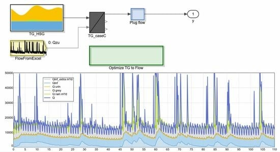
For the practical implementation of the method, the “Influent Generator 2023” block was introduced in the SIMBA^# simulation tool. The internal structure of this block is shown in Figure 8.

The dry weather inflow loads $L_{COD}$, $L_{TKN}$ and $L_P$ are specified in the dry weather block TG_HSG. The assumptions for the parameters $f_{TKN,COD,g}$, $f_{P,COD,g}$ and $TK{N}_u$ are also entered here. The measured continuous wastewater treatment plant inflow is imported from an Excel spreadsheet via the FlowFromExcel block. An algorithm is then started to adjust the shape parameters (Optimize TG to Flow block, see Figure 9).

The script block “Optimise TG” is used to determine the shape parameters of the wastewater production (the case order of the Fourier series is second: $Q_m$, $f_{Q,min}$, $T_{min}$, $f_{Q,max}$, $T_{max},$ and, the case order of the Fourier series is third: a₀..a₃, b₁..b₃), and the proportion of infiltration water is determined. Size-dependent (person equivalents—PEs) standard values are calculated for the parameters $d{T}_N$ and $\beta$.

With the now-defined dry weather inflow and the continuously measured water volume, a realistic continuous wastewater treatment plant inflow can now be calculated for a longer period of time. The calculation is performed in block TG_caseC as described in Section 2.3. This block is a so-called converter block for which the internal calculation function can be defined or altered by the user in a formula editor. This block also has a self-documentation function with which the implemented formulas can be generated as a document (see Figure 10). With this function, implemented functions are displayed transparently to the user, and the publications of models correspond exactly to the implemented function.

3. Results

3.1. Verification of the Modelling Approach for Dry Weather Inflow Pattern

This modelling approach was used to model a selection of measured example diurnal cycles. For the analysis, the data from Langergraber et al. 2008 [5] (17 examples from Austria, 2 from Germany) were supplemented by further daily profiles collected by members of the HSG Simulation working group (hsgsim.org). In particular, larger plants from Germany were included. In the presented results (see Figure 11 and Appendix C), 21 data sets from plants of wider range of sizes were analysed.

A second-order Fourier analysis was calculated to adjust the water flow rates. The analysed data sets only contain 2 h values for the water quantity; with this temporally not very high-resolution database, no significant improvement in mapping can be achieved with a higher-order Fourier series. The analysis calculates the parameters a₀, a₁, a₂, b₁ and b₂.

The parameters $Q_{inf}$ and $t_{plug}$ were optimized to adjust the $COD$ to the measured values. This means that the time series of the $COD$ concentration is completely determined by the mixture of infiltration water ($COD$ ≈ 0) and wastewater ($COD$ constant). A time shift to the time series of the water quantity and a further deformation of the pattern results from the transport through a storage volume.

The parameters $T_{N,max}$, $\beta$ and $f_{U,min}$ were optimised to adjust the $TKN$ to the measured values. The time series of the $TKN$ concentration is characterised by a proportion of $COD$, representing organic bound nitrogen, in the grey water (constant concentration) and a very high concentration (approximately 400 gN/m³) in the urine. The time function of the urine flow rate is characterised by a constant proportion ($f_{U,min} Q_{U,M}$) and a nitrogen peak in the morning $(1-f_{U,min}) Q_{U,M}$. This nitrogen peak is determined by the two shape parameters $T_{N,max}$ (time) and $\beta$ (the shape parameter of the Gumbel function and the width of the peak).

The parameter $f_{P,COD,G}$ was optimised to adjust the $P$ concentration to the measured values. Similar to the course of the $TKN$ concentration, the course of the $P$ concentration is characterised by a $COD$ proportional fraction ($f_{P,COD,G}$)) in the grey water (constant concentration) and a very high concentration in the urine. By adjusting the parameter $f_{P,COD,G}$, the pattern can be varied, with larger values of the factor in the direction of the temporal course of the $COD$ concentration, with smaller values in the direction of the pattern of the $TKN$ concentration. Unfortunately, it was only possible to adjust the $P$ concentration for a small number of measured daily patterns due to the lack of $P$ measurement values in many data sets.

This analysis impressively demonstrates that the dry weather inflow of wastewater treatment plants can be plausibly described with regard to $COD$, $TKN$ and $P$ concentrations using the simple model approach presented. The results of the analysis of all 21 daily cycles considered can be found in the appendix. Based on the analysis carried out, the systematic dependencies of the adjusted shape parameters on the plant size can also be analysed. These correlations can help to estimate typical daily patterns even for locations for which no measurements are available.

The shape parameters $T_{min}, f_{Q,min}$, $T_{max} \mathrm{and} f_{Q,max}$(for definition, see Figure 2) were determined from the time courses of the wastewater ($q_w\left(t\right)=q_u\left(t\right)+q_g\left(t\right)$). The determined shape parameters are shown in Figure 12 over the plant size in population equivalents (PE calculated from the $COD$ load with the assumption of a PE-related daily $COD$ load of 120 g $COD$/PE for raw wastewater and 78 g $COD$/PE for pre-treated wastewater (data points with red label)).

In principle, it becomes obvious from Figure 12 that the time of the night-time minimum and the morning peak are shifted backwards with the size of the system. The dynamics of the daily cycle also decrease with the size of the system, with the minimum and the maximum approaching the mean value. Despite this significant correlation, a large variance in the values can be observed. This clearly speaks in favour of the necessity of using the real measurement data of the inflow for the planning and simulation studies of wastewater treatment plants. Only in an emergency should standard assumptions be used and can be calculated with the shown linear correlations. Figure 12, bottom right, shows the height of the wastewater maximum in relation to the average wastewater volume. The examples are roughly in the range specified in DWA A198, 2003, Figure 2 [21] but also outside this range. The influence of the number of connected person equivalents (PE) to a WWTP can be summarized by two effects. For larger number of PEs, a more equalized wastewater will be the produced.For larger numbers of connected PEs, the maximum flow rate will arrive later in the day at the WWTP. These arise partly from the size of the required sewer system (more distributed sources, longer travel time). In addition, cultural differences between urban and rural areas are responsible for this behaviour. Similar results have been reported already in Langergraber et al. 2008 [5].

The $COD$ concentration time series are adjusted using the parameters $Q_{inf}$ and $t_{plug}$. There is no plausible dependence on the plant size for the infiltration water fraction. As can be seen in Figure 13 (left), the values for the proportion of extraneous water ($Q_{inf}/Q_m$ in relation to the total water volume) of the sample daily cycles fluctuate in the range of 10–70%. The temporal shift of the concentration curve in relation to the water retention volume ($t_{plug}$) varies greatly. Larger values (0.1–0.2 d) are to be expected for larger plants. Daily variations in the pre-treatment process (data points labelled in red) typically show larger delays.

Figure 14 shows the calculated $COD$ concentrations of the examples. The expected values of approximately 1000 gCOD/m³ for raw wastewater and approximately 600 gCOD/m³ for pre-treated water (data points labelled in red) are confirmed.

The $TKN$ concentration time series is adjusted to the measured values using the parameters $T_{N,max}$, $\beta$ and $f_{U,min}$. Figure 15 shows the estimated parameters over the system size. Similar to the time of the maximum inflow volume, the time of the urine peak is clearly dependent on the system size. Compared to the maximum water volume, the urine peak is between 0–0.2 d ahead (Figure 15, bottom right). The proportion of the constant urine volume varies in the range of 0.3–0.65 with outliers. There is no visible dependence on the size of the plant. Pretreated wastewater tends to produce higher values for the constant fraction of urine flow rate ($f_{U,min}$), which could be explained by further equalization in the pre-treatment stage. For the width of the urine peak ($\beta$), a dependence on the size of the plant is also visible. For larger plants, the urine flow is obviously more even, and the morning peak is less pronounced.

To adjust the phosphorus concentration pattern to the measured values, the parameter $f_{P,COD,G}$ was optimized. As only some of the available daily data contain phosphorus concentration values, a value of $f_{P,COD,G}$ = 0.008 gP/gCOD was assumed for the remaining examples. This value corresponds approximately to the mean value of the analyses for which P data was available. A correlation with the plant size is not expected and also not visible in Figure 16.

3.2. Experiences with the Method to Generate Long-Term Dynamic Simulation Influent Data

The method described here modifies the HSG method from Langergraber et al. 2008 [5] in order to improve the shortcomings described in the motivation section. This extends the scope of application of this method. For many typical municipal plants, both methods will yield comparable results. The inflow to municipal wastewater treatment plants can be described very well in most cases using both methods. The original method was used in a large number of simulation studies. The good-to-very-good agreement achieved between the simulated effluent values of the plants and the measured values is an indirect confirmation of the quality of the method.

In a simulation study carried out by the authors, the method was evaluated even further. Here, at the wastewater treatment plant, the continuous quality measurements in the influent during continuous operation (NH₄-N, online PO₄-P analyzer, daily 24 h composite samples with $COD$, $TKN$ and PO₄-P) were available. In this case, the influent data synthesized with the method could be compared with measured values. Figure 17 compares the ammonium loads calculated from the measured data with the data synthesized using the method.

A very good reproduction of the inflow situation including the rain events could be created here. Differences result primarily from variations in the inflow loads that cannot be recorded with the presented method. A quantification of the quality of a generated dynamic influent pattern as presented in Figure 17 or a quantification of the quality of achieved fit of the validated model to the available effluent measurements remains a difficult problem. There was an intensive discussion in the HSG group about the valid methods and the error definitions for this task (Ahnert et al. 2009 [23]). Simple residuals are not sufficiently significant. A visual evaluation was used here as a pragmatic solution.

The method described is not applicable in the following cases. A necessary precondition is that the dry weather inflow is mainly created from normal human activities in urbanizations (municipal wastewater). If the wastewater is completely produced by industry or a large fraction of the wastewater arises from industrial sources, the assumptions regarding cyclic production patterns of greywater and urine will not hold. The method cannot be applied. A failure of the method was also observed in one case in which municipal wastewater was pumped to the wastewater treatment plant in a widely branched pressurized pipe system with very long residence times (>4 h) (wastewater treatment plant in Berlin). In general, the method might fail in situations where large fractions of the wastewater will be managed and stored in the sewer system. This will lead to a non-predictable change in the resulting inflow patterns.

One major limitation of the method results from the assumed measurement situation (only routine data). In this situation, the influent concentration (24 h composite sample) are not measured every day but only on some days (e.g., 50 times a year). As a consequence, a constant load for every day must be assumed. Stochastic variations and typical weekly patterns cannot be reproduced. A limited quality of the influent data arises. Better influent data quality can be achieved only with an additional (non-routine) measurement effort.

But, if applicable, the method drastically reduces the requirements for influent data down to a continuous influent flow measurement and a few 24 h composite samples.

4. Summary and Outlook

In general, many simulation studies have shown that the method reproduces the particularly critical situations of incoming rain event water with a displacement load peak of wastewater stored in the sewer network by rainwater well and that the validated models reproduce the NH₄-N effluent peaks occurring at the real plants very well. This is indispensable for a capacity estimate, especially against the background of the usual monitoring practice in Germany (peak values).

In a rare number of cases, there might even be a larger data basis for modelling the available system inlet. One such special case is, for example, the availability of uninterrupted 24 h mixed samples in the inlet. In this case, an improved inflow modelling that goes beyond the method presented is theoretically possible (an imprinting of a time series of the daily inflow loads). But, due to the uncertainties in the collected data, it may also be better to use the method described here in this situation.

Another special case is the temporary availability of online measurements (e.g., NH₄-N, SAK, COD via spectrometer) in the influent of the wastewater treatment plant. In this case as well, advanced methods for inflow data generation are possible (Alex et al. 2009 [15]).

An improved modelling quality can also be achieved if diurnal variations are measured. Here, it is assumed that 12 2 h composite samples are analysed on a dry weather day in order to determine the diurnal pattern of concentration variation for COD, TKN and P. With these data, a case-specific adjustment of the shape parameters $t_{plug}$, $d{T}_N$, $\beta$, $f_{u,min}$ and $f_{P,COD,G}$ is also possible. The parameter $Q_{inf}$ can be validated or adjusted.

The method also allows an improved estimation of influent loads for wastewater treatment plants where no volume-flow-proportional 24 h-composite samples are performed (only this method normally allows reliable load calculations). Instead of volume-proportional 24 h composite samples, time-proportional 24 h composite samples are taken at many wastewater treatment plants, or only grab samples are taken. In Germany, this is partly due to the different regulations for the self-monitoring of wastewater treatment plants in the different federal states. In order to generate wastewater treatment plant inflow data for a simulation study in these situations or to estimate the inflow loads for conventional planning on a sounder basis, the following procedure can be applied. Assuming daily COD, TKN and P loads, the method can be used to synthesize a continuous course of concentrations. All types of measured values can be derived from these calculated time series, including time-proportional mixed samples or grab samples. These synthesized measured values can be compared with the real measured values. A simple search can be used to determine the loads at which the deviations between synthesized and real measured values are minimal. This provides well-founded estimates of the daily pollution loads and a reliable data set for describing the dynamic inflow of the wastewater treatment plant as a basis for model validation.

With the described method, dynamic inflow descriptions for simulation studies for municipal wastewater treatment plants can be easily generated from a few typical routine measurements. The original method (Langergraber et al. 2008 [5], Alex et al. 2009 [15]) has proven itself in many simulation studies, but the 2023 variant presented here provides comparable data and is suitable for an even broader class of applications.

In addition to generating inflow data for simulation studies, the method can also be used to generate the improved estimates of inflow loads. The required loads or volume-proportional composite concentrations can be generated from existing time-proportional composite concentrations or grab samples. This means that the method can also be used for applications beyond simulation studies, for example, for load calculation for design or benchmarking.

An emerging topic for the operation of plants is the usage of “digital twins”. One promising application are the model-based predictive controller of plants (MBPC). These MBPCs will require the online generation of reliable influent data from reliable online measurements. The method described in this paper would only require an online flow rate measurement and thus serve this specific purpose. Future research could direct in this application of the presented method.

References

- Ruiz, L.M.; Pérez, J.I.; Gómez, M.A. Practical review of modelling and simulation applications at full-scale wastewater treatment plants. J. Water Process Eng. 2023, 56, 104477. [Google Scholar] [CrossRef]
- Hvala, N.; Vrečko, D.; Levstek, M.; Bordon, C. The use of Dynamic Mathematical Models for improving the Designs of upgraded Wastewater Treatment Plants. J. Sustain. Dev. Energy Water Environ. Syst. 2017, 5, 15–31. [Google Scholar] [CrossRef]
- Gernaey, K.; van Loosdrecht, M.C.M.; Henze, M.; Lind, M.; Jørgensen, S.B. Activated sludge wastewater treatment plant modelling and simulation: State of the art. Environ. Model. Softw. 2004, 19, 763–783. [Google Scholar] [CrossRef]
- Borzooei, S.; Amerlinck, Y.; Abolfathi, S.; Panepinto, D.; Nopens, I.; Lorenzi, E.; Meucci, L.; Zanetti, M.C. Data scarcity in modelling and simulation of a large-scale WWTP: Stop sign or a challenge. J. Water Process Eng. 2019, 28, 10–20. [Google Scholar] [CrossRef]
- Langergraber, G.; Alex, J.; Weissenbacher, N.; Woerner, D.; Ahnert, M.; Frehmann, T.; Halft, N.; Hobus, I.; Plattes, M.; Spering, V.; et al. Generation of diurnal variation for influent data for dynamic simulation. Water Sci. Technol. 2008, 57, 1483–1486. [Google Scholar] [CrossRef] [PubMed]
- Ahnert, M.; Alex, J.; Dürrenmatt, D.J.; Langergraber, G.; Hobus, I.; Schmuck, S.; Spering, V. Dynamische Simulation als Bestandteil einer Kläranlagenbemessung nach DWA-A 131. KA-Korresp. Abwasser Abfall 2015, 62, 615–624. [Google Scholar]
- Alex, J.; Dürrenmatt, D.J.; Langergraber, G.; Hobus, I.; Spering, V. Voraussetzungen für eine dynamische Simulation als Bestandteil einer Kläranlagenbemessung nach DWA-A 131. KA-Korresp. Abwasser Abfall 2015, 62, 436–446. [Google Scholar]
- Juan Pablo Rodríguez, J.P.; McIntyre, N.; Díaz-Granados, M.; Achleitner, S.; Hochedlinger, M.; Maksimovi, C. Generating time-series of dry weather loads to sewers. Environ. Model. Softw. 2013, 43, 133–143. [Google Scholar] [CrossRef]
- Flores-Alsina, X.; Ort, C.; Martin, C.; Benedetti, L.; Belia Snip, L.; Saagi, R.; Talebizadeh, M.; Vanrolleghem, P.A.; Jeppsson, U.; Gernaey, K.V. Generation of (Synthetic) Influent Data for Performing Wastewater Treatment Modelling Studies. In Proceedings of the 4th IWA/WEF Wastewater Treatment Modelling Seminar, Spa, Belgium, 29 March–2 April 2014; Available online: http://www.biomath.ugent.be/WWTmod2014/ (accessed on 1 May 2023).
- Martin, C.; Vanrolleghem, P.A. Analysing, completing, and generating influent data for WWTP modelling: A critical review. Environ. Model. Softw. 2014, 60, 188–201. [Google Scholar] [CrossRef]
- Wu, X.; Zheng, Z.; Wang, L.; Li, X.; Yang, X.; He, J. Coupling process-based modeling with machine learning for long-term simulation of wastewater treatment plant operations. J. Environ. Manag. 2023, 341, 118116. [Google Scholar] [CrossRef] [PubMed]
- Ahnert, M.; Oppermann, J.; Hurzlmeier, S.; Barth, M.; Gerard, I.; Abel, T.; Bernatzky, C.; Marx, C.; Kühn, V. Das Forschungsprojekt Zeiteffiziente Analyse von Kläranlagen (ZAK)—Von der Idee zum Produkt. In Abwasser Abfall; DWA: Hennef, Germany, 2014; pp. 124–130. [Google Scholar]
- Arbeitsblatt, A.D.A. 131—Bemessung von Einstufigen Belebungsanlagen; DWA: Hennef, Germany, 2016. [Google Scholar]
- Hauduc, H.; Gillot, S.; Rieger, L.; Ohtsuki, T.; Shaw, A.; Takacs, I.; Winkler, S. Activated sludge modelling in practice: An international survey. Water Sci. Technol. 2009, 60, 1943–1951. [Google Scholar] [CrossRef] [PubMed]
- Alex, M.; Hetschel, M. Ogurek: Simulation Study with Minimized Additional Data Requirements to Analyse Control and Operation of WWTP Dorsten, Water Science & Technology; IWA Publishing: London, UK, 2009. [Google Scholar]
- Mannina, G.; Cosenza, A.; Vanrolleghem, P.A.; Viviani, G. A practical protocol for calibration of nutrient removal wastewater treatment models. J. Hydroinform. 2011, 13, 575–595. [Google Scholar] [CrossRef]
- Almeida, M.C.; Butler, D.; Friedler, E. At-source domestic wastewater quality. Urban Water 1999, 1, 49–55. [Google Scholar] [CrossRef]
- Flores-Alsina, X.; Saagi, R.; Lindblom, E.; Thirsing, C.; Thornberg, D.; Gernaey, K.V.; Jeppsson, U. Calibration and validation of a phenomenological influent pollutant disturbance scenario generator using full-scale data. Wat. Res. 2013, 51, 172–185. [Google Scholar] [CrossRef] [PubMed]
- SIMBA#. SIMBA# Water 5.0 User Manual; ifak e.V. Magdeburg: Magdeburg, Germany; Available online: https://www.ifak.eu/de/produkte/simba (accessed on 1 May 2023).
- Gernaey, K.V.; Flores-Alsina, X.; Rosen, C.; Benedetti, L.; Jeppsson, U. Dynamic influent pollutant disturbance scenario generation using a phenomenological modelling approach. Environ. Model. Softw. 2011, 26, 1255–1267. [Google Scholar] [CrossRef]
- Arbeitsblatt, A.D.A. 198—Vereinheitlichung und Herleitung von Bemessungswerten für Abwasseranlagen; DWA: Hennef, Germany, 2003. [Google Scholar]
- Rojas, K.; Galvis, A.; Schütze, M. Modelling of sediments in the drainage system of Cali/Colombia. In Proceedings of the 14th International Conference on Urban Drainage, Prague, Czech Republic, 10–15 September 2017. [Google Scholar]
- Ahnert, M.; Blumensaat, F.; Langergraber, G.; Alex, J.; Woerner, D.; Frehmann, T.; Halft, N.; Hobus, I.; Plattes, M.; Spering, V.; et al. Goodness-of-fit measures for numerical modelling in urban water management—A review to support practical applications. In Proceedings of the LWWTP07 Conference, Vienna, Austria, 9–13 September 2007; pp. 69–72. [Google Scholar]
Figure 1.
Modelling approach for dry weather inflow Langergraber et al. 2008 [5].
Figure 2.
Fourier approximation of the dry weather inflow Langergraber et al. 2008 [5].
Figure 3.
Dry weather influent block in SIMBA#.
Figure 4.
Setting the shape parameters.
Figure 5.
Setting the concentrations.
Figure 6.
Inlet flow data with dry weather period.
Figure 7.
Inlet divided into additional infiltration water, infiltration water, urine, grey water, and rainwater runoff.
Figure 8.
Inflow calculation in the SIMBA block “Influent Generator 2023”.
Figure 9.
Automatic adjustment of the form parameters.
Figure 10.
Self-documentation from block TG_caseC.
Figure 11.
Reproduction of daily pattern, variant 2023 (selection). The legends for measured Q and measured COD include the id (1–21) of the analysed sample plant. See Appendix C for all analysed data sets.
Figure 12.
Shape parameter wastewater flow rate as a function of plant size (PE). (A linear regression line is plotted as grey dotted line which appears as solid grey line in the plots).
Figure 13.
Shape parameter COD pattern. (A linear regression line is plotted as grey dotted line which appears as solid grey line in the plots).
Figure 14.
Resulting concentrations in the wastewater. (A linear regression line is plotted as grey dotted line which appears as solid grey line in the plots).
Figure 15.
Shape parameter for TKN pattern. (A linear regression line is plotted as grey dotted line which appears as solid grey line in the plots).
Figure 16.
Shape parameter P pattern. (A linear regression line is plotted as grey dotted line which appears as solid grey line in the plots).
Figure 17.
Synthetic inflow data (NH4-N load in kg/d) compared with measured data.