
Stratospheric Water Vapor from the Hunga Tonga–Hunga Ha’apai Volcanic Eruption Deduced from COSMIC-2 Radio Occultation

 ,
,  ,
,  , and
, and 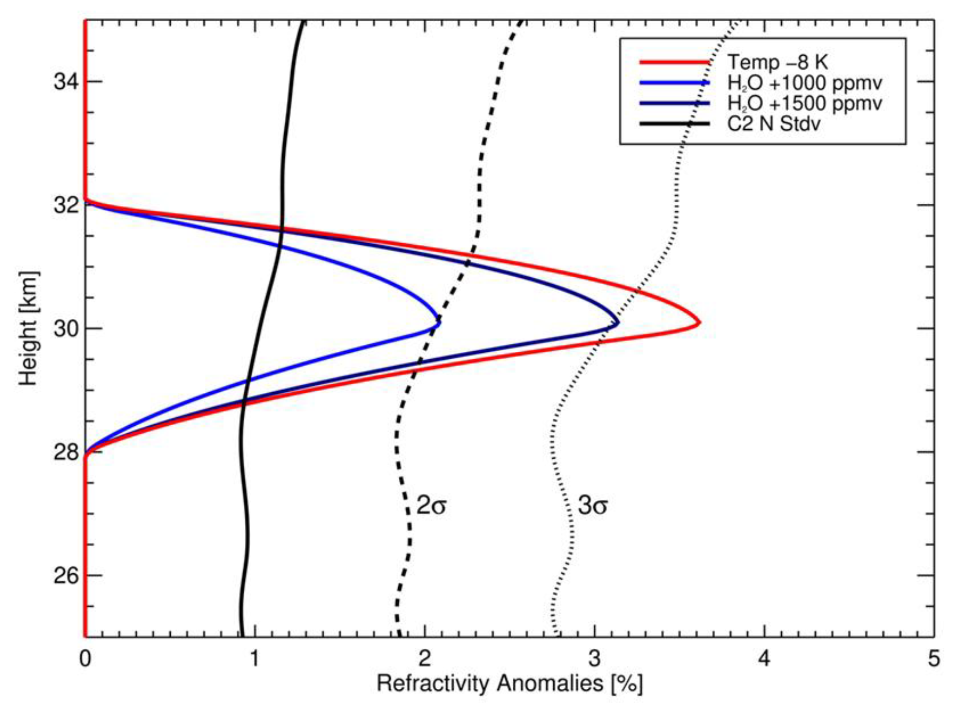
Abstract
:1. Introduction
2. Materials and Methods
- (a)
- C2 GNSS-RO observations
- (b)
- MLS temperatures
- (c)
- Radiosondes
3. Results
3.1. RO Sensitivity to Stratospheric H2O
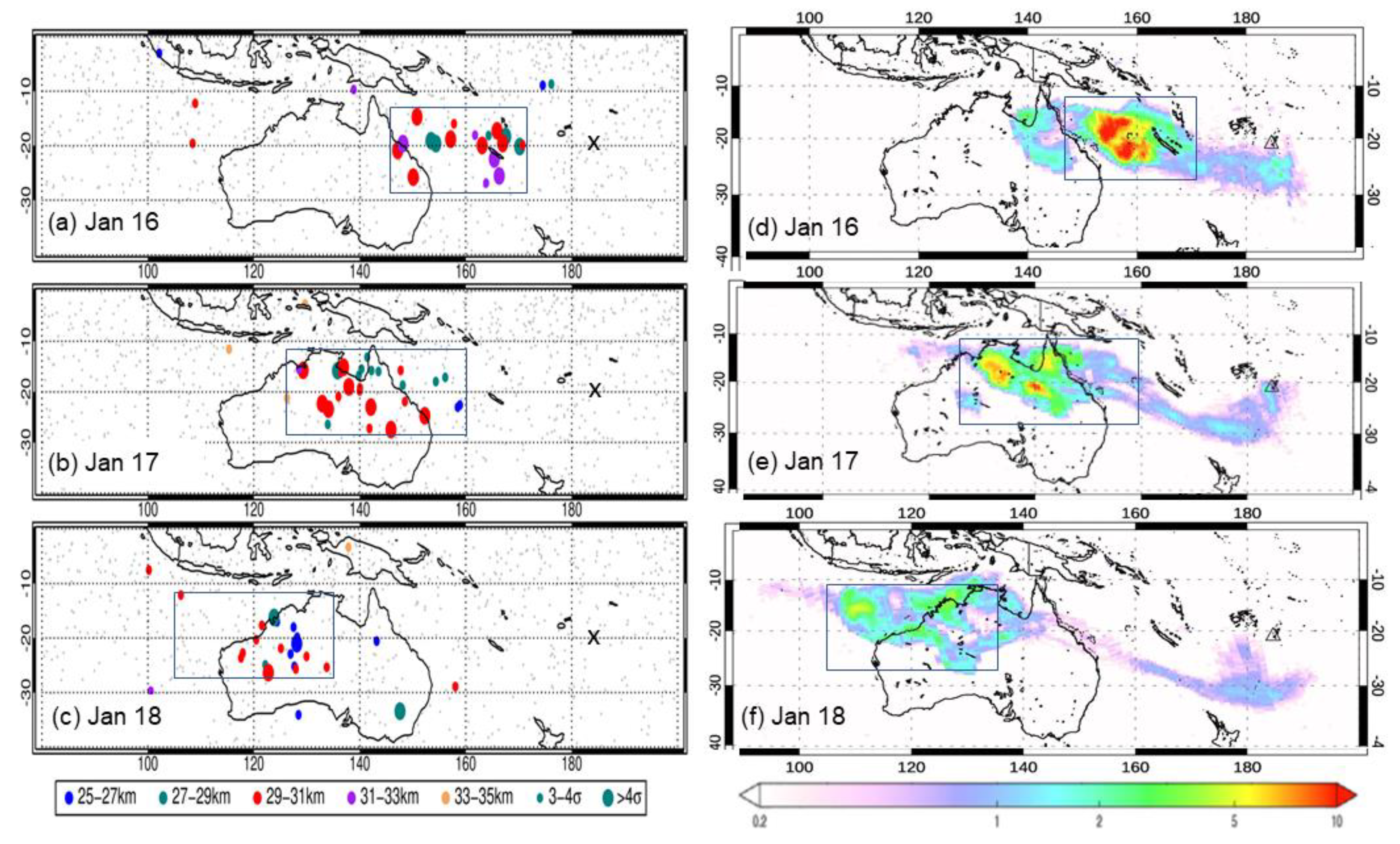
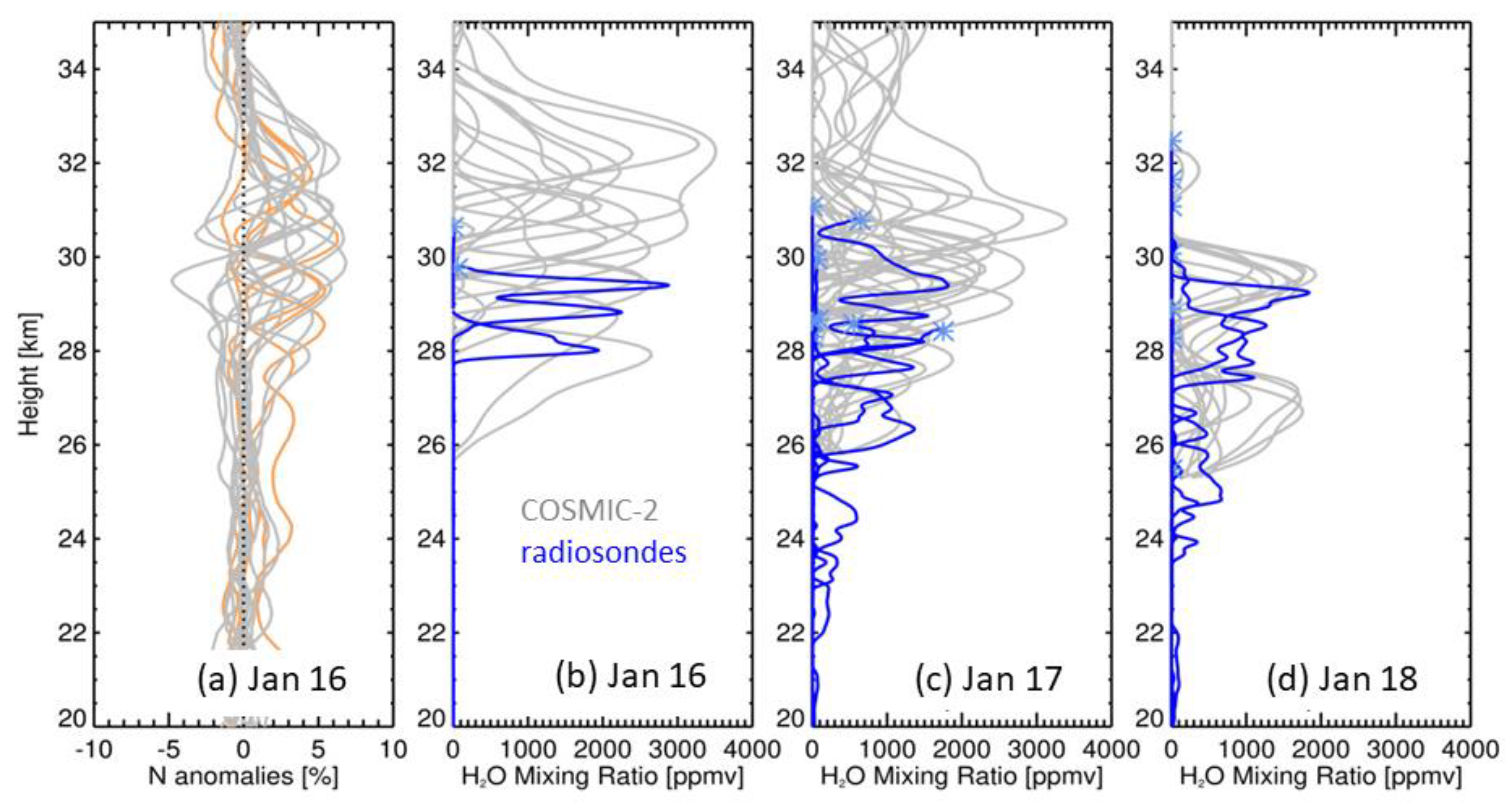
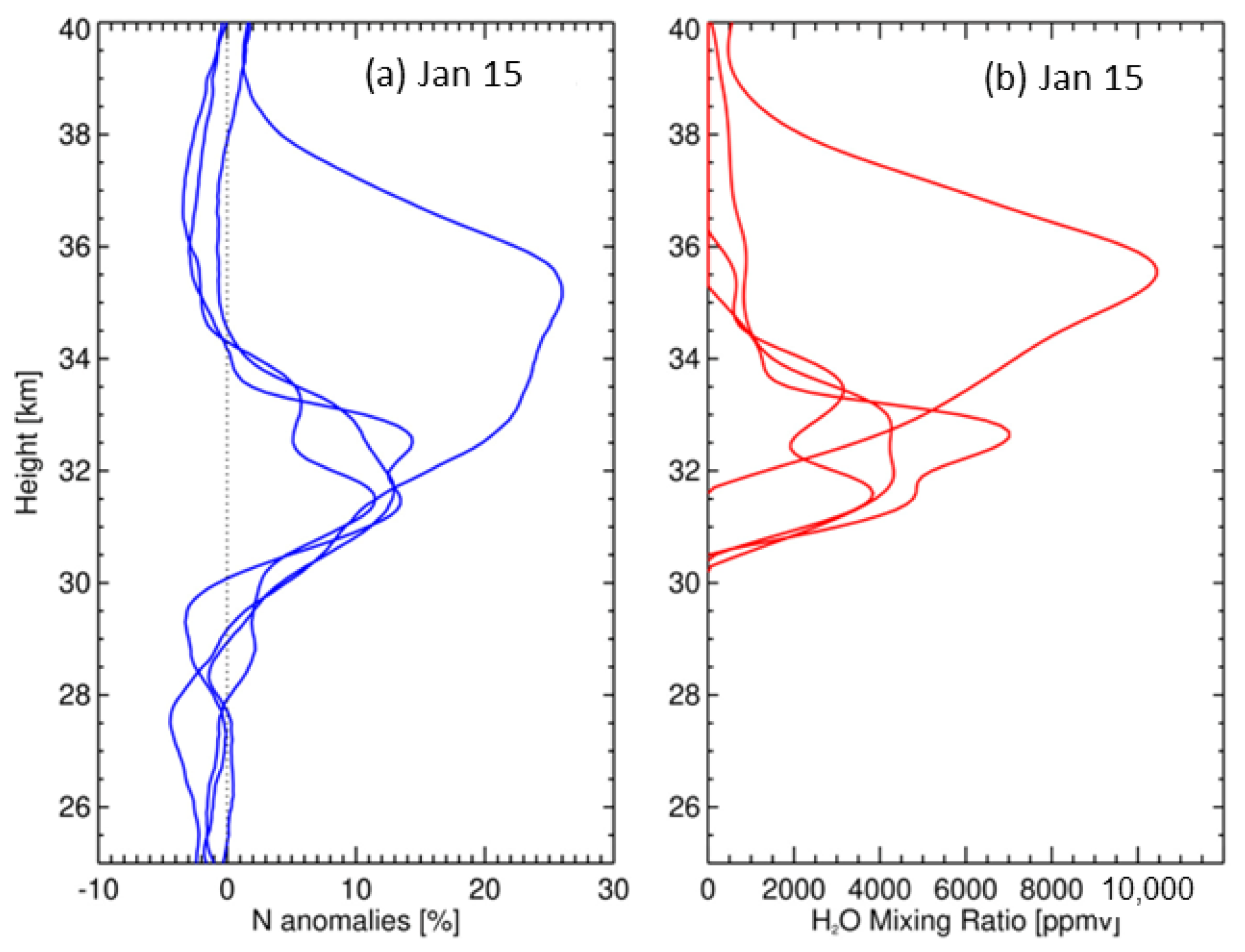
3.2. C2 HTHH Refractivity Observations and H2O Retrievals
3.3. Mass of H2O in the Early HTHH Plume
4. Discussion
Author Contributions
Funding
Data Availability Statement
Acknowledgments
Conflicts of Interest
Appendix A. Retrieval of Water Vapor from Radio Occultation Refractivity and Ancillary Temperature Data


References
- Sellitto, P.; Podglajen, A.; Belhadji, R.; Boichu, M.; Carboni, E.; Cuesta, J.; Duchamp, C.; Kloss, C.; Siddans, R.; Bègue, N.; et al. The unexpected radiative impact of the Hunga Tonga eruption of 15th January 2022. Commun. Earth Environ. 2022, 3, 288. [Google Scholar] [CrossRef]
- Vömel, H.; Evan, S.; Tully, M. Water vapor injection into the stratosphere by Hunga Tonga-Hunga Ha’apai. Science 2022, 377, 1444–1447. [Google Scholar] [CrossRef] [PubMed]
- Khaykin, S.; Podglajen, A.; Ploeger, F.; Grooß, J.-U.; Tence, F.; Bekki, S.; Khlopenkov, K.; Bedka, K.; Rieger, L.; Baron, A.; et al. Global perturbation of stratospheric water and aerosol burden by Hunga eruption. Commun. Earth Environ. 2022, 3, 316. [Google Scholar] [CrossRef]
- Millán, L.; Santee, M.L.; Lambert, A.; Livesey, N.J.; Werner, F.; Schwartz, M.J.; Pumphrey, H.C.; Manney, G.L.; Wang, Y.; Su, H.; et al. The Hunga Tonga-Hunga Ha'apai Hydration of the Stratosphere. Geophys. Res. Lett. 2022, 49, e2022GL099381. [Google Scholar] [CrossRef] [PubMed]
- Xu, J.; Li, D.; Bai, Z.; Tao, M.; Bian, J. Large Amounts of Water Vapor Were Injected into the Stratosphere by the Hunga Tonga–Hunga Ha’apai Volcano Eruption. Atmosphere 2022, 13, 912. [Google Scholar] [CrossRef]
- Legras, B.; Duchamp, C.; Sellitto, P.; Podglajen, A.; Carboni, E.; Siddans, R.; Grooß, J.-U.; Khaykin, S.; Ploeger, F. The evolution and dynamics of the Hunga Tonga–Hunga Ha’apai sulfate aerosol plume in the stratosphere. Atmos. Chem. Phys. 2022, 22, 14957–14970. [Google Scholar] [CrossRef]
- Schoeberl, M.R.; Wang, Y.; Ueyama, R.; Taha, G.; Jensen, E.; Yu, W. Analysis and impact of the Hunga Tonga-Hunga Ha'apai stratospheric water vapor plume. Geophys. Res. Lett. 2022, 49, e2022GL100248. [Google Scholar] [CrossRef]
- Carr, J.L.; Horváth, Á.; Wu, D.L.; Friberg, M.D. Stereo Plume Height and Motion Retrievals for the Record-Setting Hunga Tonga-Hunga Ha’apai Eruption of 15 January 2022. Geophys. Res. Lett. 2022, 49, e2022GL098131. [Google Scholar] [CrossRef]
- Ravindra Babu, S.; Lin, N.-H. Extreme Heights of 15 January 2022 Tonga Volcanic Plume and Its Initial Evolution Inferred from COSMIC-2 RO Measurements. Atmosphere 2023, 14, 121. [Google Scholar] [CrossRef]
- Anthes, R.A.; Bernhardt, P.A.; Chen, Y.; Cucurull, L.; Dymond, K.F.; Ector, D.; Healy, S.B.; Ho, S.-P.; Hunt, D.C.; Kuo, Y.-H.; et al. The COSMIC/FORMOSAT-3 Mission: Early Results. Bull. Am. Meteorol. Soc. 2008, 89, 313–333. [Google Scholar] [CrossRef]
- Smith, E.K.; Weintraub, S. The Constants in the Equation for Atmospheric Refractive Index at Radio Frequencies. Proc. IRE 1953, 41, 1035–1037. [Google Scholar] [CrossRef]
- Kursinski, E.R.; Hajj, G.A.; Schofield, J.T.; Linfield, R.P.; Hardy, K.R. Observing Earth's atmosphere with radio occultation measurements using the Global Positioning System. J. Geophys. Res. 1997, 102, 23429–23465. [Google Scholar] [CrossRef]
- Zeng, Z.; Sokolovskiy, S.; Schreiner, W.S.; Hunt, D. Representation of Vertical Atmospheric Structures by Radio Occultation Observations in the Upper Troposphere and Lower Stratosphere: Comparison to High Resolution Radiosonde Profiles. J. Atmos. Ocean. Technol. 2019, 36, 655–670. [Google Scholar] [CrossRef]
- Livesey, N.J. Aura Microwave Limb Sounder (MLS) Version 4.2x Level 2 and 3 Data Quality and Description Document. 2018. Available online: http://mls.jpl.nasa.gov/ (accessed on 20 November 2018).
- Johnston, B.R.; Randel, W.J.; Braun, J.J. Interannual Variability of Tropospheric Moisture and Temperature and Relationships to ENSO using COSMIC-1 GNSS-RO Retrievals. J. Clim. 2022, 35, 3509–3525. [Google Scholar] [CrossRef]
- Carn, S.A.; Krotkov, N.A.; Fisher, B.L.; Li, C. Out of the blue: Volcanic SO2 emissions during the 2021–2022 eruptions of Hunga Tonga—Hunga Ha’apai (Tonga). Front. Earth Sci. 2022, 10, 976962. [Google Scholar] [CrossRef]
- Hersbach, H.; Bell, B.; Berrisford, P.; Hirahara, S.; Horányi, A.; Muñoz-Sabater, J.; Nicolas, J.; Peubey, C.; Radu, R.; Schepers, D.; et al. The ERA5 global reanalysis. Quart. J. R. Meteor. Soc. 2020, 146, 1999–2049. [Google Scholar] [CrossRef]
- Wang, X.; Randel, W.; Zhu, Y.; Tilmes, S.; Starr, J.; Yu, W.; Garcia, R.; Toon, B.; Park, M.; Kinnison, D.; et al. Stratospheric climate anomalies and ozone loss caused by the Hunga Tonga volcanic eruption. Authorea, 2022; preprint. [Google Scholar] [CrossRef]
- Pitari, G.; Mancini, E. Short-term climatic impact of the 1991 volcanic eruption of Mt. Pinatubo and effects on atmospheric tracers. Nat. Hazards Earth Syst. Sci. 2002, 2, 91–108. [Google Scholar] [CrossRef]


Disclaimer/Publisher’s Note: The statements, opinions and data contained in all publications are solely those of the individual author(s) and contributor(s) and not of MDPI and/or the editor(s). MDPI and/or the editor(s) disclaim responsibility for any injury to people or property resulting from any ideas, methods, instructions or products referred to in the content. |
© 2023 by the authors. Licensee MDPI, Basel, Switzerland. This article is an open access article distributed under the terms and conditions of the Creative Commons Attribution (CC BY) license (https://creativecommons.org/licenses/by/4.0/).
Share and Cite
Randel, W.J.; Johnston, B.R.; Braun, J.J.; Sokolovskiy, S.; Vömel, H.; Podglajen, A.; Legras, B. Stratospheric Water Vapor from the Hunga Tonga–Hunga Ha’apai Volcanic Eruption Deduced from COSMIC-2 Radio Occultation. Remote Sens. 2023, 15, 2167. https://doi.org/10.3390/rs15082167
Randel WJ, Johnston BR, Braun JJ, Sokolovskiy S, Vömel H, Podglajen A, Legras B. Stratospheric Water Vapor from the Hunga Tonga–Hunga Ha’apai Volcanic Eruption Deduced from COSMIC-2 Radio Occultation. Remote Sensing. 2023; 15(8):2167. https://doi.org/10.3390/rs15082167
Chicago/Turabian StyleRandel, William J., Benjamin R. Johnston, John J. Braun, Sergey Sokolovskiy, Holger Vömel, Aurelien Podglajen, and Bernard Legras. 2023. "Stratospheric Water Vapor from the Hunga Tonga–Hunga Ha’apai Volcanic Eruption Deduced from COSMIC-2 Radio Occultation" Remote Sensing 15, no. 8: 2167. https://doi.org/10.3390/rs15082167