Article

Risk Assessment and Analysis of Its Influencing Factors of Debris Flows in Typical Arid Mountain Environment: A Case Study of Central Tien Shan Mountains, China

1
Key Laboratory of Mountain Hazards and Surface Process, Institute of Mountain Hazards and Environment, Chinese Academy of Sciences, Chengdu 610041, China
2
College of Engineering, Tibet University, Lhasa 850012, China
3
Faculty of Public Safety and Emergency Management, Kunming University of Science and Technology, Kunming 650093, China
4
Academy of Plateau Science and Sustainability, Xining 810016, China
5
Kathmandu Center for Research and Education, Chinese Academy of Sciences-Tribhuvan University, Beijing 100101, China
6
University of Chinese Academy of Sciences, Beijing 100049, China
7
Department of Civil Engineering, International University of Business Agriculture and Technology (IUBAT), Dhaka 1230, Bangladesh
8
Department of Civil Engineering, Kunsan National University, Gunsan 54150, Republic of Korea
*
Author to whom correspondence should be addressed.
Remote Sens. 2023, 15(24), 5681; https://doi.org/10.3390/rs15245681
Submission received: 12 October 2023 / Revised: 30 November 2023 / Accepted: 6 December 2023 / Published: 11 December 2023

Abstract

:
The Tien Shan Mountain range connects Central Asia with northwestern China and is a crucial transport junction between East and West Asia. It is a common location for regional debris flows, which pose a significant risk to ecological security and the safety of people and property. Nevertheless, limited knowledge exists about the distribution of disaster risks and the impacted populations. This study uses advanced machine learning techniques to identify the key natural and social factors influencing these hazards and incorporates the Social Vulnerability Index (SoVI) to assess societal vulnerability. The outcomes demonstrate that (1) the debris flow hazard in the Tien Shan Mountain area is primarily governed by the geological structure, which dictates the material source and, in turn, dictates the onset of debris flows. (2) The vulnerability demonstrates a high spatial tendency in the north and a low one in the south, with evident spatial clustering characteristics. (3) A total of 19.13% of the study area is classified as high-hazard, with specific distribution zones including the northern foothills of the Tien Shan Mountains, the low-mountain zones of the southern foothills of the Tien Shan Mountains, and the Yili Valley zone. This holistic approach offers valuable insights into the spatial distribution of risks, aiding in prioritizing disaster preparedness and mitigation efforts. Also, our findings and conclusions are beneficial for local decision makers to allocate resources effectively and promote sustainable development practices in the region.

1. Introduction

Debris flows are a common hazard in mountainous regions and are one of the most serious geological hazards causing casualties and damage worldwide [1]. From 1950 to 2011, 213 debris flows occurred globally, leading to 77,779 fatalities [2]. These hazards are immense, posing severe threats to human lives and properties and causing extensive damage to crucial infrastructure [3]. The Tien Shan Mountains (TSMs) are situated in the inner part of the Asia–Europe continent, subject to the squeezing effect of the Asia–Europe continent and the Indian Ocean plate, with an active geological structure, rugged landforms and diversified climatic types, and is an important transport and economic corridor between China and Central Asia. With the implementation of strategies such as the “China-Pakistan Economic Corridor”, “The Silk Road”, and “Western Development”, the TSMs and the surrounding region will be significant for strategic transport, oil, and gas pipelines and the establishment of towns and settlements. Together with the increase in extreme precipitation in recent years [4], there has been an increase in strong seismic activity, the number of earthquakes [4,5], and engineering disturbances. As a result, the TSM region is vulnerable to severe debris flow disasters. Therefore, it is crucial to quantitatively assess the risk of debris flow in the TSM region, particularly in climate change, to prioritize the urgent need for regional economic development and human safety.
Debris flow hazard mapping is a crucial component of effective land-use planning in debris flow-prone areas, providing quickly interpretable information for the identification of vulnerable regions and the prioritization of mitigation strategies. At present, methods for assessing and zoning debris flow disaster hazard can be summarized into several categories. (1) Hazard zoning can be determined by frequency and scale, such as by delineating zones based on historical records and observations. However, field observations are hindered by the harsh natural environment and the high cost of construction. (2) Multi-criteria decision-making techniques, such as hierarchical analysis [6], have limitations in terms of objectivity due to their reliance on subjective hierarchical scoring. (3) On the other hand, statistical and bivariate-based models [7] like the frequency ratio, informativeness, coefficient of certainty, weight of evidence, fuzzy logic, etc. also have their limitations. These methods are restricted by linear assumptions and low-order attributes, and may not provide a high degree of precision when applied to high-dimensional data. (4) Mathematical–physical models [8], such as finite element, discrete element, and finite volume methods based on the theory of continuous and discontinuous media, were used. However, the modeling and physical parameter preparation require significant labor and are only appropriate for a small scale. With the advent of 3 s technology and computers, machine learning techniques are increasingly utilized to assess geological hazards. Numerous scholars have considered various factors before adopting machine learning algorithms to partition the study area into hazard zones. This approach has yielded better results mainly because ML learns from the data, simplifies the relationship between variables in the data through statistical modeling, and compensates for the shortcomings of traditional methods, including a large workload, strong subjectivity, and low prediction accuracy [9]. Furthermore, given the vast amounts of geoscience data, machine learning can provide a massively effective way to manage information. Although the use of machine learning methods for evaluating the susceptibility of geohazards at a global level is increasingly prevalent, as previously noted, there is still much to be explored regarding the use of these techniques for assessing debris flow susceptibility in all aspects.
Debris flows are known to occur due to a variety of factors including geomorphologic, climatic and tectonic forces such as differences in the altitude, gradient, precipitation and density of faults. These different elements interplay and contribute towards the occurrence of debris flows. However, numerous recent studies and cases demonstrate that drought can directly impact the hydromechanical and mechanical properties of soil. This can cause an increase in cracks and the formation of dominant seepage channels. Additionally, it can lead to the “air resistance” effect of the soil body, hindering water seepage and making the surface layer of the soil more prone to paralyzed sliding [1]. These theories regarding the impact of “drought” on debris flow disasters have been substantiated by numerous actual cases. For instance, the disastrous ZSDF in Ganluo County in 2019, which occurred within the arid valley area of the Hengduan Mountains [10], and comparable illustrations can be found in the Tianshan Mountains of China [11]. The Tianshan region, with an average annual precipitation of 170.62 mm and evapotranspiration in the range of 523–1528 mm, represents a classic arid region within Asia and Europe. However, the causes of regional debris flows in arid climates, including the main controlling factors, remain unclear at this stage. Consequently, machine learning was employed to identify the main controlling factors of debris flows in arid regions.
Previous research on debris flows in the TSMs has primarily concentrated on analyzing debris flows at a single gully scale [12,13,14,15], including the gully tectono-geomorphologic investigation, disaster event’s parameter calculation, and mitigation method planning. Yet, the establishment of a region-wide debris flow database and debris flow hazard and risk assessment are still lacking. The debris flow risk is determined by a combination of hazard attributes and social attributes, and many areas initially considered to be low-hazard have resulted in casualties due to the neglect of the link between hazards and human society. How to effectively synthesize hazard attributes and social attributes to assess the debris flow risk is a topic worth exploring. When considering the implications of debris flows on society lives and properties vulnerability is a frequently used proxy of societal attributes, as it reflects the extent of harm caused to individuals by debris flow hazards. Many experts have attempted to quantify and represent vulnerability with a variety of methods. For instance, Lo [16] has introduced a flowchart to create a building vulnerability curve that evaluates the damage caused by debris flow hazards to buildings. Winter [17], on the other hand, has developed a curve function that estimates the vulnerability of debris flows to roads by collecting questionnaire survey reports that depend on expert judgments of quantitative probabilities. However, it is not feasible to utilize these approaches to quantify regional scale’s vulnerability, and other methods or indicators are needed to achieve this goal. Meanwhile, the Social Vulnerability Index (SoVI) is an effective indicator, appraising and measuring social vulnerability broadly. Yet, although SoVI has been widely used in other disaster risk assessments, it has not yet been applied to debris flow. Here, we employ SoVI as a vulnerability proxy for the first time to assess debris flow risk in the TSMs, a positive and beneficial exploration in debris flow risk assessments.
Risk was defined by the United Nations Department of Humanitarian Affairs (DHA) in 1992 as “the expected value of the loss of human life, property and economic activity due to a natural hazard in a given area and over a given period of time”. Therefore, risk is equal to the product of hazard and vulnerability [18]. Here, this study aims to clarify the key controlling factors of debris flow spatial distribution using a machine learning technique in the TSMs. Additionally, the Social Vulnerability Index will be incorporated to evaluate regional debris flow risk, combined with debris flow hazard assessments. This paper addresses the following inquiries: (1) What are the main factors that determine the distribution of debris flows in the TSMs? (2) How are hazards and vulnerabilities spatially distributed in the TSMs? (3) What are the spatially differentiated debris flow risks in the TSMs? The results of this research can be used to improve the standard of disaster prevention and mitigation and support government planning, decision making, and ecological development.
This research makes a significant scientific contribution by comprehensively analyzing debris flow hazards in the TSMs. It identifies the key natural and social factors influencing these hazards and incorporates the SoVI to assess societal vulnerability. This holistic approach offers valuable insights into the spatial distribution of risks, aiding in prioritizing disaster preparedness and mitigation efforts. The findings have direct policy implications and can inform decision makers, helping them allocate resources effectively and promote sustainable development practices in the region, ultimately enhancing safety and resilience in the face of debris flow disasters.

2. Materials and Methods
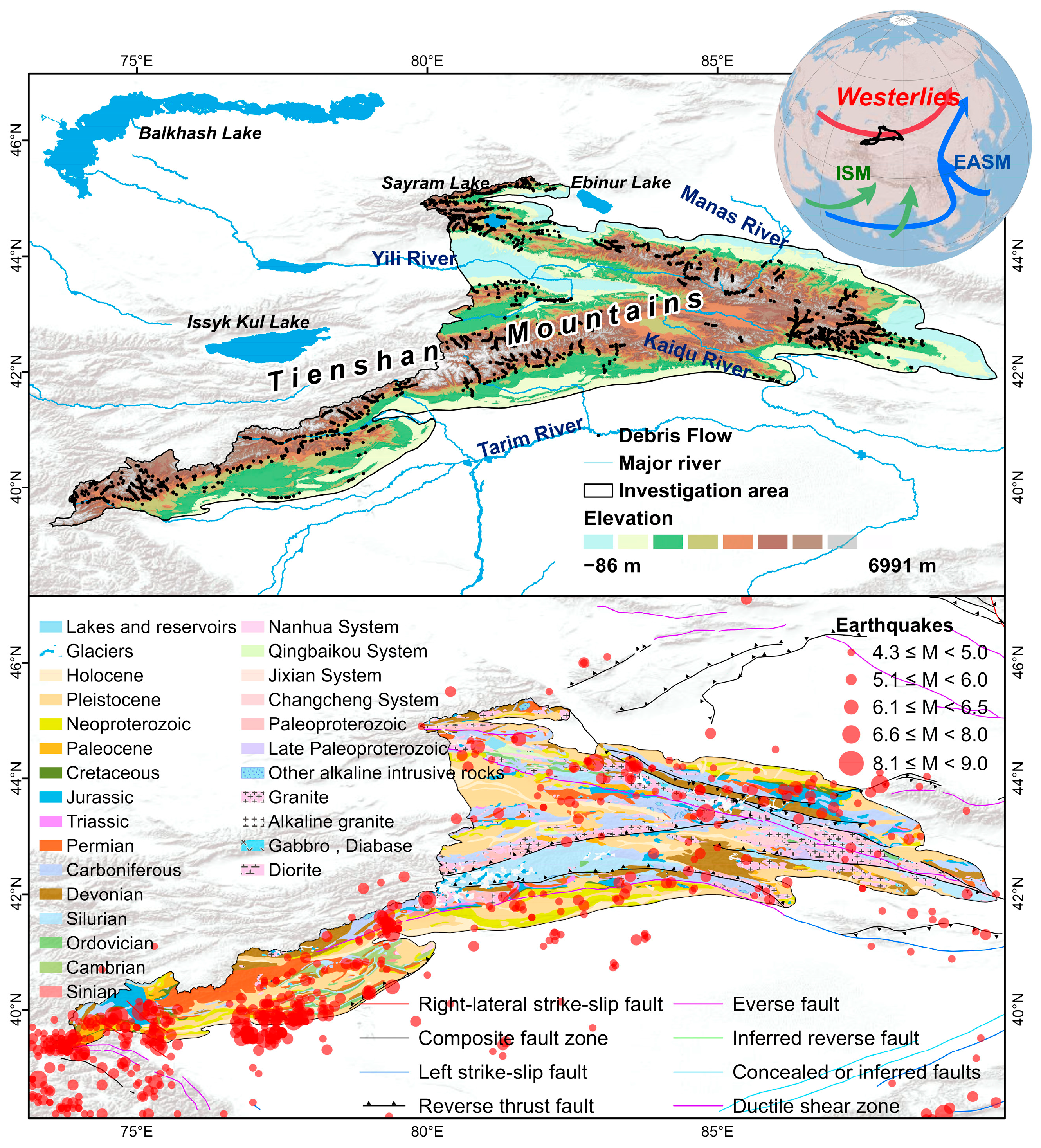
2.1. Study Area

The TSMs are the most visually varied inland mountainous area in Central Asia, covering more than 2.5 million km2. They also serves as a socioeconomic hub of the region (Figure 1). During their formation, the TSMs underwent a Late Paleozoic–Permian uplift to shape the Paleotian Mountains, Mesozoic and Early Tertiary uplifts, and the New Tertiary uplift of the Himalayan Movement, culminating in an arrangement of mountain ranges intertwined with basins [19,20,21]. Numerous Cenozoic basins formed due to both latitudinal and Cenozoic faulting. Moreover, the TSMs uplift at 1–80 mm/a, while the Junggar Basin sinks at a rate of 10 mm/a [22]. Seismic activity is frequent in the region, with a generally VII–VIII-degree intensity. Since 1900, over 35 earthquakes of magnitude VI have occurred, with the Manas earthquake in 1906 causing large casualties [23]. Additionally, the TSM region experiences significant small-earthquake activity. From 2000 to 2022, more than 10,000 earthquakes of magnitude 1–5 have occurred in the study area.
The westerly winds influence the regional climate in the TSMs [24]. Recent analyses of temperature observations and simulations indicate a temperature change rate of 0.34 °C/10a, which is greater than the Northern Hemisphere and global averages during the same period [25]. From 1961 to 2013, the average temperature increase was 0.32 °C per decade. The temperature rise was more substantial on the southern slopes of the TSMs compared to the northern ones, with the eastern and western sections experiencing higher temperatures than the central region. The precipitation also showed a fluctuating growth trend, with an average increase of 10.32 mm per decade. The annual rainfall in the foothill area of the northern slope of TSMs amounts to approximately 400 mm, while the average precipitation in the southern slope is around 200 mm. Moreover, regional precipitation rises with increasing altitude; the highest precipitation altitude zone is approximately 3000 m. The regional rainfall is also greater than that on the southern slope of TSMs [26]. The intricate geological and climatic conditions have resulted in numerous debris flow disasters in the TSMs, including the 6 August 1970 overturning of train 2522 [27]. Other disasters include the Kuitun River debris flow on 15 July 1987, which resulted in the destruction of the recently repaired water diversion project with a loss of 20 million pounds, and the Aragou debris flow in the same year, which buried several factories and mines in the Nanshan mining area of Urumqi, rendering thousands of people homeless [28].

2.2. Data Source and Pre-Processing

The debris flow disaster data was obtained from the inventory of debris flow disaster locations established by the relevant departments in the Xinjiang Province, including the previous historical debris flow disaster locations and the debris flow disaster locations obtained from the survey work in a small area of the region. Based on this, a preliminary screening of debris flows using remote sensing analysis was carried out. Field visits were carried out between September and October 2020, and July and August 2021, to authenticate and validate the identification of debris flow disaster points using remote sensing images. The resultant database comprising 2097 debris flows was used as the model input. We employed the watershed as our unit of analysis, with various input factors, and applied machine learning algorithms and SoVI to establish a hazard and vulnerability assessment model. Using the product of debris flow hazard and vulnerability, we developed the debris flow risk assessment model. Please refer to Figure 2 for the study’s flow chart.
Accurate evaluation plays a crucial role in regional geohazard risk assessment, and selecting appropriate evaluation factors can enhance the assessment’s precision. Studies have indicated that three categories of factors significantly influence debris flow hazard assessment, namely loose material sources, abundant water sources, and steep topography. Similarly, we considered the three dimensions of exposure, capability of coping and resilience in selecting the factors for the vulnerability assessment. In summary, taking into account the results of previous relevant studies and field surveys, we selected a total of 22 risk assessment factors from various aspects such as geomorphology, geology, hydrology and socio-economics. The hazard assessment utilizes 13 factors, including the catchment area, elevation difference, gradient, topographical relief, lithological intensity, fault density, peak ground acceleration, land cover, topographic wetness index, normalized vegetation index, road density, average annual rainfall, and normalized snow index. The vulnerability assessment utilizes 9 factors, including the population density, building density, economic density, road density, number of hospital beds per million people, percentage of the population aged over 64 years, percentage of the population aged under 14 years, GDP per capita, and the proportion of the labor force of the appropriate age. Table 1 displays the data sources and formats for each factor.
After collecting the above data, we carried out a series of data preprocessing steps, including the digitization of data products, rasterization of elements, stitching, projection transformation, resampling and cropping [29]. Eventually, we obtained the dataset under the WGS84 coordinate system. As some factors’ raw data are type quantities, they necessitate conversion into numerical values for model input. Land cover reflects the intensity of soil and water loss in a region, which in turn affects the amount of material carried by debris flows when they occur. Therefore, any human intervention in the land cover, including ecological damage, can cause and increase debris flow hazards [30]. Land cover types vary considerably in their surface infiltration rates and erosion resistance. To address this, a table of land cover type classification indicators was compiled from previous research studies [31,32] (Table 2). The stratigraphic lithology indicates the main source of debris flow material. Additionally, broken rock enters the channel and replenishes the debris flow source. Based on the study [29,33], the lithology of the study area is categorized into four types: very soft rock, soft rock, hard rock, and very hard rock, based on the engineering geological rock group (Table 3). After this, we utilized the zoning statistics tool of ArcGIS (https://www.esri.com/zh-cn/home (accessed on 15 May 2022)) to calculate the factor values for watershed units for the hazard assessment factor, which were then normalized and input into the machine learning model. Regarding the vulnerability factor, we evaluated administrative divisions and conducted a principal component analysis after normalizing the data.

2.2.1. Tests of Covariance for Hazard Assessment Variables

The 13 hazard evaluation factors listed in Table 1 were chosen according to the characteristics of the hazard-prone environment in the region and past studies [29,34]. However, it is unnecessary to include more factors as this may increase the modeling error due to potential multi-collinearity [35,36]. Therefore, conducting a covariance test on the 13 selected factors is necessary. The covariance analysis utilized tolerance (TOL) and VIF values. Typically, the results suggest that TOL <= 0.1 and VIF > 10 [37] indicate extensive multicollinearity issues.

2.2.2. Variable of Vulnerability Assessment

Vulnerability assessment necessitates consideration of a variety of factors. We assessed distinctions in socioeconomic and cultural traits and datasets and opted for nine socioeconomic factors to measure vulnerability. The nine factors can be grouped into exposure, capability of coping, and resilience.
In the event of a disaster, human exposure is the primary concern, especially for individuals residing in mountainous regions, who commonly live on debris flow and landslide accumulation fans and are more susceptible to harm. Population density: The potential for maximum loss of life is correlated with population density [38,39]. Densely populated areas are more vulnerable to debris flows and have greater exposure than sparsely populated areas.
Building density: The level of regional building congestion and the hierarchy of spatial structures directly impact building density. Debris flow damage threatens artificial structures, and vulnerability is closely linked to building density [40]. The more extensive the building density, the greater the severity of the damage caused by debris flow.
Economic vulnerability can be assessed through GDP, which comprehensively gauges a region’s economic development, social prosperity, and capacity to recuperate from a disaster [41]. Regions with higher GDPs experience higher economic losses and greater vulnerability to debris flows.
Economic density: Road density is another factor to consider [41]. Roads are a significant transportation infrastructure which often intersect or traverse geohazard-prone areas, such as mountainous regions and river valleys. Debris flows, which are prone to occur, can lead to road destruction or blockages, and a higher road density increases vulnerability.
The number of hospital beds per 10,000 is a crucial economic indicator for healthcare organizations [42]. The greater the number of beds available at a healthcare facility, the greater the number of patients it can accommodate, the broader range of medical services it can offer, and the greater capacity it has to respond to emergencies in the event of a disaster.
The percentage of the population aged over 64 years: the Seventh Census reveals a general decline in birth rates in recent years, highlighting the issue of population aging [43]. The elderly population is particularly vulnerable to disasters [44], and according to international census criteria, individuals over the age of 64 are classified as elderly, while those under 14 are classified as pre-pubescent. Older households are more susceptible to hazards. Retired adults and preadolescents tend to spend more time indoors than other age groups for various reasons related to work, physical ability, and physiology. This population may have slower reaction times, fewer opportunities to escape debris flows, and slower disaster recovery. In addition, preadolescent children and older adults are more susceptible to injuries, disabilities, and fatalities resulting from debris flows, thus rendering them more vulnerable than their counterparts in other age groups [45]. In consideration of the preceding points, we have included the proportion of the population aged 64 and over as one of the variables.
Percentage of the population aged under 14 years: Similar to those over 64, children under 14 are also considered vulnerable. Therefore, the proportion of the population under 14 years old was utilized as one of the variables [40].
Gross Domestic Product (GDP) per Capita [41]: GDP per capita serves as a universally accepted measure of economic development, objectively reflecting the high living standards of individuals within a region. Higher GDP per capita implies improved material infrastructure, a higher level of social development, and stronger disaster resistance and adaptive capacity. Furthermore, a higher GDP per capita in post-disaster recovery can offer a stronger guarantee for economic reconstruction and social stability.
We must also consider the proportion of the labor force of the appropriate age. Some studies have suggested that gender differences cause varying perceptions of debris flows [46]. However, the most recent study in the Salween Valley region found that males and females share similar perceptions of the debris flow threat [45]. It additionally confirms that younger individuals possess a higher level of perception about risk than their elder counterparts.

2.3. Methods

2.3.1. Methods of Hazard Assessment

Breiman proposed Random Forest (RF) based on integration and is an integrated learning model comprising multiple decision trees [47]. As a data-driven non-parametric classification method, RF uses CART clusters for predictive classification. The random sampling technique is utilized to create clusters of regression trees by sampling a portion of the training sample set with put-back, and the final classification results are obtained by voting. The sample set is randomly partitioned into various training and test sets. About two-thirds of the training samples (in-bag samples) will train the regression tree, whereas the remaining one-third (out-of-bag samples) will be reserved for internal validation. This will assist in estimating the error in classifying results from the Random Forest classifier. Compared to other machine learning techniques, Random Forest exhibits high prediction accuracy, quick convergence, and substantial mitigation against the effects of “overfitting”. As such, in this paper, negative sample data of 2097 “non-debris flow” units were chosen randomly in the study area based on the number of identified debris flows. Using the random forest model, we then established a regression equation to assess debris flow hazard, with the debris flow hazard as the target variable and the independent variables being the positive and negative sample data and the influencing factor.

2.3.2. Methods of Vulnerability Assessment

The Social Vulnerability Index (SoVI) assesses social vulnerability to hazards on a regional scale. Cutter proposed the SoVI in 2003 to compare UK regions’ vulnerability [48]. Socioeconomic and demographic factors significantly affect susceptibility, and the SoVI aids understanding of the reasons for varied human capacity to prepare for, respond to, and recover from disasters.
We applied Principal Component Analysis (PCA) to reduce nine variables into fewer, more significant components [39]. We utilized varimax rotation to decrease variables with more substantial loadings on individual factors, resulting in greater independence between factors. We adopted Keiser’s criterion to determine and keep components with eigenvalues exceeding one. When the validation of the SoVI is not feasible, it is crucial to assess the resilience of the SoVI. This involves examining the effect of scale modifications on SoVI scores and their distribution [49]. We employed Kaiser–Meyer–Olkin (KMO) and Bartlett’s sphericity tests to determine if the principal component analysis yielded acceptable outcomes. We then added the principal components to compute the SoVI index for the designated research region.

2.3.3. Methods of Risk Assessment

We calculated risk using the United Nations definition of risk [18]. Hazard and vulnerability were both normalized values on a scale of 0 to 1.
R = H × V
where R is the degree of risk (0–1), H is the degree of hazard (0–1), and V is the vulnerability (0–1).

3. Results

3.1. Debris Flow Hazard Assessment in the TSMs

Based on Table 4, it can be concluded that there is a notable covariance problem between Slope and RDLS. Furthermore, we generated a correlation heat map utilizing the Pearson coefficient (Figure 3). Based on the literature [36], the Slope factor with a high correlation of Pearson = 0.98 should have been excluded. After analyzing both VIF and Pearson results, we excluded the Slope factor and utilized only 12 remaining factors as inputs for the following model. The spatial distribution of these factors is displayed in Figure 4.
Assessing model performance is a crucial aspect of debris flow hazard modeling. To ensure the model’s accuracy, we utilized the receiver operating characteristic curve (ROC) for evaluation. The ROC has been extensively employed to verify geological hazard prediction models [50]. The area under the curve (AUC) provides a quantitative measure of model accuracy, with values ranging from 0.5 to 1.0. Higher AUC values correspond to a better model performance. The closer the AUC is to 1, the more accurate the model is. AUC values within the 0.5–0.6, 0.6–0.7, 0.7–0.8, 0.8–0.9, and 0.9–1.0 range can be classified as poor, average, good, very good, and excellent. The AUC was calculated based on the prediction scores. The average AUC after ten cross-validations was 0.88 (Figure 5). This is an indication that the random forest models have adequate predictive ability.
Based on the Natural Breaks (Jenks) method, the TSM watershed hazard was classified into five hazard categories: low, slight, moderate, high, and very high (Figure 6). The sub-areas with extraordinarily high and high susceptibility are mainly located in the Borohoro Mountains, western Eren Habirga Shan, northern Halik Mountains, Narat Shan, eastern Ketmen Range, Sary Jaz Mountains, Terskey Ala-too, and Kakshaal Too.
Analyzed from the standpoint of topographic and geomorphological patterns, areas of extreme and high hazard are primarily situated in the pre-mountainous area, with high rates of erosion and weathering and a dry climate, as well as the mountainous region, covering roughly 70,151.28 km2, which constitutes 33% of the entire area. The specific traits of loess deposition zones in the pre-mountainous regions render them susceptible to destructive debris flows, particularly evident in the low hills of southern Huocheng County, Yining County, Yining City, and other nearby areas. Additionally, the mountains of south Zhaosu County, southern Tekes County, southern Xinyuan County, and northern Huocheng County are considered at a high hazard of debris flows.
We generated box plots to investigate the correlation between influencing factors and debris flow hazards in the TSM region (Figure 7). The plots demonstrate the relationship between different debris flow hazard class types and various factors. Six factors, namely fault density, topographic relief, normalized difference snow index, average annual precipitation, elevation difference, and catchment area, have a notable positive correlation with the hazard class. The correlation results show that as the value of the factor increases, so does the hazard. One noteworthy observation is that a smaller catchment area may pose a greater hazard, suggesting the occurrence of significant disasters in smaller watersheds within the study zone [10]. There is no discernible linkage between vegetation coverage and land utilization. The hazard of debris flows is higher in areas with lower TWI, potentially due to steeper slopes in mountainous regions, which provide more energy for debris flow initiation. Hard-rock areas are more susceptible to debris flows and pose greater danger than soft-rock areas. The hazard of debris flows is elevated in regions with high levels of peak ground acceleration. The relationship between road density and debris flow danger suggests that areas with less human activity are more prone to high-hazard debris flows. This is likely because glacial-type debris flows present greater danger and occur farther from road locations [51]. In summary, the geological structure largely determines the debris flow hazard in the TSM area.

3.2. Debris Flow Vulnerability Assessment in the TSMs

Vulnerability refers to the extent of damage caused by the disaster agent [52,53,54]. Regional vulnerability was evaluated using PCA to analyze the nine socioeconomic factors outlined earlier to derive the Social Vulnerability Index (SoVI). SoVI, a measure of vulnerability, was calculated by inputting the nine socioeconomic variables through PCA analysis.
The results are presented in Table 5 and Figure 8, where an eigenvalue > 1 was selected as the principal component to simplify the nine variables into three principal components. Bartlett’s test of sphericity was calculated, with a highly significant p-value of <0.01, and KMO was found to be 0.610. Both of these results indicate that the principal component analysis is reliable. The variance differences between the principal components are maximized through varimax rotation, facilitating the interpretation of the principal components [39] (refer to Table 6). Demographic factors (PC1 = 35.21%) were identified as the most significant factor in interpreting the dominant SoVI, followed by economic factors (PC2 = 27.56%) and resilience factors (PC3 = 15.53%). These three principal components together explain 78.3% of the total variables. The initial factor comprises demographics, encompassing the proportion of seniors over 64 [45], population under 14, and population density. Following this is the economic factor, which covers total GDP, building, and economic density. Lastly, the resilience factor is accounted for, which considers the number of hospital beds per 10,000, road density, and proportion of the labor force of the appropriate age.
Global spatial autocorrelation analysis and spatial visualization of the three principal components revealed that the population and resilience factors were spatially clustered, and the clustering was statistically significant based on the p-values (Figure 9). Most of the population is concentrated in the northern part of the study area because it is located in the North Slope Economic Zone of Xinjiang, which accounts for only 5.7% of the province of Xinjiang but 23.3% of the total population [55]. Regions with high economic factors are mainly located in several small but economically developed districts and counties, and the distribution shows a negative spatial correlation according to the Moran index, but a p-value > 0.05 indicates that the negative correlation is not significant. The strong resilience region is located in the central plains region, which is consistent with the study that concluded that the plains region has stronger resilience than the mountains [56].
The SoVI is formulated as the total of the main components, weighted by their respective percentage variances. The formula for SoVI is determined using the three principal components mentioned earlier in this text, as follows:
SoVI = ((35.208 × PC1)/78.326) + ((27.586 × PC2)/78.326) + ((15.533 × PC3)/78.326)
where PC1\PC2\PC3 are three principal components.
The vulnerability findings are presented in Figure 10, depicting the geographical allocation of vulnerability on the district scale. The most susceptible regions are in the West and North East, comprising Dushanzi, Saybag, Yining City, Korla, and Changji City. These areas constitute 10.8% of the population and possess substantial economic development, thereby explaining the elevated level of vulnerability. Notwithstanding the abundance of healthcare resources, transportation accessibility, and disaster resilience, these factors have minimal impact on reducing vulnerability. The areas with the lowest susceptibility are situated in the South (Artux, Xinhe, Shufu, Marabishi, Aketao, Kalpin, Payzawat) and the Center (Tekes). These eight regions (17.4%) exhibit low susceptibility primarily due to their small population and relatively underdeveloped economy despite their weak resilience to disasters.
The vulnerability test using the global Moran’s index exhibited a value of 0.278 with a p-value of 0.006, less than 0.01, and a z-value of 2.9189, which exceeds 2.58 through Geoda software1.14 (https://geodacenter.github.io/ (accessed on 12 July 2023)). This finding suggests a considerable positive spatial correlation in the overall vulnerability of the 46 cities at the county level in the region. In simpler terms, the neighboring regions’ SoVI indicates a “high-high concentration” or “low-low concentration” spatial concentration.

3.3. Debris Flow Risk Assessment in the TSMs

Debris flow risk relates to the influence of natural characteristics on social attributes and is an essential prerequisite for emergency response to disasters [57]. After separate calculations of the hazard and vulnerability, the risk level of debris flows in the TSMs was determined (Figure 11). The calculation results indicate that the high-risk region spans approximately 7828.67 km2, making up 3.68% of the total area, and the higher-risk region spans about 32,840.65 km2, accounting for 15.45% of the total area. In addition, we divided the high-risk regions of the TSMs into three concentrated distribution zones. Firstly, the low-mountain zone along the northern foothills of the TSMs, including Bole City, Jinghe County, Wusu City, Shawan County, Manas County, Hutubi County, and Changji City. Secondly, the low-mountain zone along the southern foothills of the TSMs, including Hejing County, northern Wensu County, northern Baicheng County, northern Kuqa City, north of Bugur County, and Aheqi County. Lastly, the Yili Valley zone includes Khorgas, Qorghas, Yining County, Yining City, and southern Xinyuan County.
The risk level of the low-mountain belt along the northern foothills of the TSMs is higher than the remaining two concentrated belts. This is due to two factors. Firstly, the foothills of the north are situated at a higher level in the hazard assessment. Secondly, the northern foothills of the TSMs are the economic belt of the slopes of the north of the TSMs, where vulnerability is also maintained at a high level, thus establishing the high-risk characteristics of the foothills of the north of the TSMs.
We validated debris flow risk assessment through field surveys and visits (Figure 12). For instance, the G30 highway frequently experiences temporary disruptions caused by debris flows (Figure 12c1,c2) [58]. In July 2022, during a field survey, a dangerous debris flow occurred in Maoliu Gully on the G217 highway, resulting in a 12 h interruption of the G217 highway and posing a severe threat to social development. Overall, the findings of the field survey were consistent with the evaluation.

4. Discussion

Central Asia, part of the TSM range, experiences significant debris flow hazards. For instance, Bassam, Tajikistan, witnessed glacial debris flows due to heavy rainfalls and increased temperatures caused by global warming [8]. In addition, glacial debris flows and moraine-dammed glacial lakes in the mountainous areas of southeastern Kazakhstan pose a greater future threat [15]. These occurrences may also be found in the Kyrgyzstan’s Central TSM plateau’s Ak-Shiirak range [59]. The Andes and the TSMs constitute a semi-arid mountain range [60] characterized by extensive glaciers and similar topographic and geomorphological features. Nonetheless, limited research has been conducted on the risk of debris flow in the Andes and the five Central Asian countries. Therefore, we utilized the TSM area as a case study to investigate the formation mechanisms of debris flows in arid zones, with the expectation that we can enrich the theoretical study of debris flow hazards in arid zones (Central Asia, Andes, etc.). This article used various data sources to evaluate the risk of debris flows in the TSM area. Our study revealed that the primary factor instigating debris flows is fault density. Additionally, we discovered that tectonic activity causes rivers to erode quickly, leading to a high frequency of landslides that can potentially trigger debris flows [61]. For instance, landslides offset 75% of the tectonic uplift caused by the 2008 Wenchuan earthquake, while 12.76% of the deposited material flowed into river channels and became debris flows [62]. Developed tectonics leads to a higher density of faults, which leads to an increase in the number of sources, and ultimately to a greater susceptibility to debris flow initiation, especially in seismic arid-semiarid regions such as the TSMs. Furthermore, the initiation of debris flows is affected by external dynamics like climate change, freeze–thaw cycles, and extreme rainfall. We conclude that physical sources are responsible for initiating debris flows in the TSM region, primarily due to geological processes controlling their initiation and their significant interplay with hydrological processes [3]. Next, we suggested an on-going or future conceptual map to express the whole process of debris flow risk in the TSM arid region from the perspective of the debris flow formation mechanism (Figure 13), with the expectation that the conceptual map in this paper and the assessment of debris flow risk in the TSMs can provide some implications for the five Central Asian countries as well as the Andes.
Debris flows within the TSM range may become increasingly threatening due to global warming and frequent climate extremes. The retreat of glaciers and the degradation of moraines have led to the creation of additional loose accumulations, like the Gangotri Glacier debris flow in the Himalayas that was triggered by an increase in such accumulations [63]. The accelerated melting of snow and ice due to global warming has resulted in the increased formation of runoff [60], making water hazards such as flash floods and debris flows more likely to occur. In addition to the melting of snow and ice, heavy rainfall resulting from extreme weather is also a crucial mechanism for triggering debris flows in the future. In addition, studies indicate that the combination of more rain and less snowfall caused by global warming, particularly in high-altitude mountains, will worsen the severity of heavy rainfall [64]. This, in turn, increases the likelihood of landslides and debris flows. Furthermore, population growth and urban expansion will heighten the vulnerability of areas to debris flows [65]. Hence, high-hazard and high-vulnerability regions may encounter long-term, high-risk issues.
This study enhances the theoretical debris flow disaster risk assessment methods and provides scientific references for effective debris flow prevention and control. Nonetheless, it has some limitations. Firstly, although the Social Vulnerability Index performs better when describing regional large-scale vulnerability, it does not effectively describe local small-scale vulnerability [38]. As socio-economic statistics become more accurate and their resolution improves, this problem will be effectively resolved. Secondly, the spatial pattern of risk calculation is derived solely from past data, hence uncertainties and limitations may exist in the evaluation results regarding climate change. As time progresses, the risk of debris flows, and socioeconomic vulnerability will also change, owing to the changes in environmental conditions and societal development. Thus, future studies must consider risk mapping across a range of time frames.

5. Conclusions

The TSM region is characterized by its mountainous terrain and specific geographical location, resulting in frequent geological disasters threatening residents’ livelihoods, production, and ecological safety. Considering the regional context of debris flow occurrences and the unique topography and geomorphology of TSMs, we conducted a comprehensive assessment of the potential risk of debris flows in the area. The risk assessment comprises two elements: firstly, constructing a hazard assessment that depicts the natural attributes of the disaster, and secondly, conducting a vulnerability assessment that represents the social attributes. To accomplish this, we utilized machine learning techniques to evaluate the hazard using 12 debris flow risk factors on a watershed unit. Random forests were employed to measure the hazard and compute the factors’ contribution. The debris flow vulnerability assessment incorporated nine socioeconomic factors, which were downscaled using the PCA method to three principal components: demographic, economic, and resilience. The risk of debris flows across the TSMs area was analyzed based on the formula determining risk as the multiplication of vulnerability and hazard. The results show the following:
  • The hazard of debris flows in the Tien Shan region results from geological and tectonic processes. The tectonics determine the source material, which in turn controls the initiation of debris flows. The density of faults, topographic relief, and differences in height are the primary factors that affect the likelihood of debris flows in Tien Shan.
  • The Tien Shan region exhibits a spatial pattern of high vulnerability in the north and low vulnerability in the south. The neighboring regions’ SoVI also displays positive spatial autocorrelation, characterized by evident spatial clustering features.
  • A total of 19.13% of the Tien Shan region is categorized as high-risk, divided into three distribution zones: the low-mountain zone in the Tien Shan’s northern foothills, the low-mountain zone along the southern foothills of the Tien Shan, and the Yili Valley zone. Monitoring and early warning in these three areas are crucial.

Author Contributions

N.C. and Z.L. conceived the original ideas and drafted the original manuscript. R.H., S.T., M.W. and M.R. conducted field investigation and collected data. N.C. and Z.L. revised the original manuscript. All authors have read and agreed to the published version of the manuscript.

Funding

This research was funded by the Second Tibetan Plateau Scientific Expedition and Research Program (STEP) of China (GrantNo. 2019QZKK0902) and National Key Research and Development Program of China (Grant No. 2023YFC3008301) and Special Research Assistant Grant of the Chinese Academy of Sciences (Grant Recipient: Dr. Shufeng Tian) and the National Natural Science Foundation of China (Grant Nos. U20A20110) and the International Cooperation Overseas Platform Project, CAS (Grant No. 131C11KYSB20200033).

Data Availability Statement

Data are contained within the article.

Acknowledgments

We would like to thank the reviewers and the editors for their constructive comments. We also thank to the data support from “National Earth System ScienceData Center, National Science & Technology Infrastructure of China (http://www.geodata.cn, accessed on 20 March 2023).

Conflicts of Interest

The authors declare no conflict of interest.

References

  1. Chen, N.; Tian, S.; Zhang, Y.; Wang, Z. Soil mass domination in debris-flow disasters and strategy for hazard mitigation. Earth Sci. Front. 2021, 28, 337–348. [Google Scholar] [CrossRef]
  2. Dowling, C.A.; Santi, P.M. Debris Flows and Their Toll on Human Life: A Global Analysis of Debris-Flow Fatalities from 1950 to 2011. Nat. Hazards 2014, 71, 203–227. [Google Scholar] [CrossRef]
  3. Tian, S.; Hu, G.; Chen, N.; Rahman, M.; Han, Z.; Somos-Valenzuela, M.; Habumugisha, J.M. Extreme Climate and Tectonic Controls on the Generation of a Large-Scale, Low-Frequency Debris Flow. Catena 2022, 212, 106086. [Google Scholar] [CrossRef]
  4. Zhang, X.; Chen, Y.; Fang, G.; Li, Y.; Li, Z.; Wang, F.; Xia, Z. Observed Changes in Extreme Precipitation over the Tienshan Mountains and Associated Large-Scale Climate Teleconnections. J. Hydrol. 2022, 606, 127457. [Google Scholar] [CrossRef]
  5. Zhu, S.; Liang, H.; Wei, W.; Li, J. Slip rates and seismic moment deficits on major faults in the Tianshan region. Seismol. Geol. 2021, 43, 249–261. [Google Scholar]
  6. Tie, Y.; Tang, C. Application of AHP in single debris flow risk assessment. Chin. J. Geol. Hazard Control 2006, 17, 79–84. [Google Scholar]
  7. Sun, Y.; Ge, Y.; Chen, X.; Zeng, L.; Liang, X. Risk Assessment of Debris Flow along the Northern Line of the Sichuan-Tibet Highway. Geomat. Nat. Hazards Risk 2023, 14, 2195531. [Google Scholar] [CrossRef]
  8. Yılmaz, K.; Dinçer, A.E.; Kalpakcı, V.; Öztürk, Ş. Debris Flow Modelling and Hazard Assessment for a Glacier Area: A Case Study in Barsem, Tajikistan. Nat. Hazards 2023, 115, 2577–2601. [Google Scholar] [CrossRef]
  9. Merghadi, A.; Yunus, A.P.; Dou, J.; Whiteley, J.; ThaiPham, B.; Bui, D.T.; Avtar, R.; Abderrahmane, B. Machine Learning Methods for Landslide Susceptibility Studies: A Comparative Overview of Algorithm Performance. Earth-Sci. Rev. 2020, 207, 103225. [Google Scholar] [CrossRef]
  10. Tian, S.; Chen, N.; Rahman, M.; Hu, G.; Peng, T.; Zhang, Y.; Liu, M. New Insights into the Occurrence of the Catastrophic Zhaiban Slope Debris Flow That Occurred in a Dry Valley in the Hengduan Mountains in Southwest China. Landslides 2022, 19, 647–657. [Google Scholar] [CrossRef]
  11. Chen, Y.; Chou, J.; Zhang, H. Activity characters of rainstion mudflow in arid land—Taking Ala creek Tianshan Mountains as Example. Jouranl Arid. Land Resour. Environ. 1991, 5, 43–48. [Google Scholar] [CrossRef]
  12. Passmore, D.G.; Harrison, S.; Winchester, V.; Rae, A.; Severskiy, I.; Pimankina, N.V. Late Holocene Debris Flows and Valley Floor Development in The Northern Zailiiskiy Alatau, Tien Shan Mountains, Kazakhstan. Arct. Antarct. Alp. Res. 2008, 40, 548–560. [Google Scholar] [CrossRef]
  13. Lv, L.Q.; Chen, N.S.; Lu, Y.; Huang, Q.; Li, J.; Zhu, Y.H. Characteristics and Mechanics Analysis of Debris Flow Disaster in Xinjiang Arid Area. Adv. Mater. Res. 2012, 594–597, 2318–2322. [Google Scholar] [CrossRef]
  14. Winchester, V.; Passmore, D.G.; Harrison, S.; Rae, A.; Severskiy, I.; Pimankina, N.V. Dendrogeomorphological and Sedimentological Analysis of Debris Flow Hazards in the Northern Zailiiskiy Alatau, Tien Shan Mountains, Kazakhstan. In Vulnerability of Land Systems in Asia; Braimoh, A.K., Huang, H.Q., Eds.; John Wiley & Sons, Ltd.: Chichester, UK, 2014; pp. 91–113. ISBN 978-1-118-85494-5. [Google Scholar]
  15. Medeu, A.R.; Popov, N.V.; Blagovechshenskiy, V.P.; Askarova, M.A.; Medeu, A.A.; Ranova, S.U.; Kamalbekova, A.; Bolch, T. Moraine-Dammed Glacial Lakes and Threat of Glacial Debris Flows in South-East Kazakhstan. Earth-Sci. Rev. 2022, 229, 103999. [Google Scholar] [CrossRef]
  16. Lo, W.-C.; Tsao, T.-C.; Hsu, C.-H. Building Vulnerability to Debris Flows in Taiwan: A Preliminary Study. Nat. Hazards 2012, 64, 2107–2128. [Google Scholar] [CrossRef]
  17. Winter, M.G.; Smith, J.T.; Fotopoulou, S.; Pitilakis, K.; Mavrouli, O.; Corominas, J.; Argyroudis, S. An Expert Judgement Approach to Determining the Physical Vulnerability of Roads to Debris Flow. Bull. Eng. Geol. Environ. 2014, 73, 291–305. [Google Scholar] [CrossRef]
  18. Sun, R.; Gao, G.; Gong, Z.; Wu, J. A Review of Risk Analysis Methods for Natural Disasters. Nat. Hazards 2020, 100, 571–593. [Google Scholar] [CrossRef]
  19. Ji, J.; Luo, P.; White, P.; Jiang, H.; Gao, L.; Ding, Z. Episodic Uplift of the Tianshan Mountains since the Late Oligocene Constrained by Magnetostratigraphy of the Jingou River Section, in the Southern Margin of the Junggar Basin, China. J. Geophys. Res. Solid. Earth 2008, 113, B05102. [Google Scholar] [CrossRef]
  20. Yang, S.; Li, J.; Wang, Q. The Deformation Pattern and Fault Rate in the Tianshan Mountains Inferred from GPS Observations. Sci. China Ser. D-Earth Sci. 2008, 51, 1064–1080. [Google Scholar] [CrossRef]
  21. Wu, C.; Zhang, P.; Zhang, Z.; Zheng, W.; Xu, B.; Wang, W.; Yu, Z.; Dai, X.; Zhang, B.; Zang, K. Slip Partitioning and Crustal Deformation Patterns in the Tianshan Orogenic Belt Derived from GPS Measurements and Their Tectonic Implications. Earth-Sci. Rev. 2023, 238, 104362. [Google Scholar] [CrossRef]
  22. Abdrakhmatov, K.Y.; Aldazhanov, S.A.; Hager, B.H.; Hamburger, M.W.; Herring, T.A.; Kalabaev, K.B.; Makarov, V.I.; Molnar, P.; Panasyuk, S.V.; Prilepin, M.T.; et al. Relatively Recent Construction of the Tien Shan Inferred from GPS Measurements of Present-Day Crustal Deformation Rates. Nature 1996, 384, 450–453. [Google Scholar] [CrossRef]
  23. Wang, C.-Y.; Yang, Z.-E.; Luo, H.; Mooney, W.D. Crustal Structure of the Northern Margin of the Eastern Tien Shan, China, and Its Tectonic Implications for the 1906 M~7.7 Manas Earthquake. Earth Planet. Sci. Lett. 2004, 223, 187–202. [Google Scholar] [CrossRef]
  24. Li, G.; Wang, X.; Zhang, X.; Yan, Z.; Liu, Y.; Yang, H.; Wang, Y.; Jonell, T.N.; Qian, J.; Gou, S.; et al. Westerlies-Monsoon Interaction Drives out-of-Phase Precipitation and Asynchronous Lake Level Changes between Central and East Asia over the Last Millennium. Catena 2022, 218, 106568. [Google Scholar] [CrossRef]
  25. Chen, Y.; Li, W.; Deng, H.; Fang, G.; Li, Z. Changes in Central Asia’s Water Tower: Past, Present and Future. Sci. Rep. 2016, 6, 35458. [Google Scholar] [CrossRef] [PubMed]
  26. Yao, J.; Chen, Y.; Guan, X.; Zhao, Y.; Chen, J.; Mao, W. Recent Climate and Hydrological Changes in a Mountain–Basin System in Xinjiang, China. Earth-Sci. Rev. 2022, 226, 103957. [Google Scholar] [CrossRef]
  27. Yan, X. The Administration of Debris flow in Alagou Basin of Tianshan. Arid Land Geograpyh 1991, 68–75. [Google Scholar] [CrossRef]
  28. Qiao, M.; Wang, Z.; Yang, F.; Li, W. Classification and Type Character of Debris flow Along Alago River Basin of Tianshan Mountains in Xinjiang. Arid Land Geograpyh 1991, 68–75. [Google Scholar] [CrossRef]
  29. Zhou, Y.; Yue, D.; Liang, G.; Li, S.; Zhao, Y.; Chao, Z.; Meng, X. Risk Assessment of Debris Flow in a Mountain-Basin Area, Western China. Remote Sens. 2022, 14, 2942. [Google Scholar] [CrossRef]
  30. Turner, B.; Meyer, W.B.; Skole, D.L. Global Land-Use/Land-Cover Change: Towards an Integrated Study. Ambio A J. Human. Environ. 1994, 23, 91–95. [Google Scholar]
  31. Efthimiou, N.; Psomiadis, E. The Significance of Land Cover Delineation on Soil Erosion Assessment. Environ. Manag. 2018, 62, 383–402. [Google Scholar] [CrossRef]
  32. Sharma, A.; Tiwari, K.N.; Bhadoria, P.B.S. Effect of Land Use Land Cover Change on Soil Erosion Potential in an Agricultural Watershed. Environ. Monit. Assess. 2011, 173, 789–801. [Google Scholar] [CrossRef] [PubMed]
  33. Li, Y.; Wang, H.; Chen, J.; Shang, Y. Debris Flow Susceptibility Assessment in the Wudongde Dam Area, China Based on Rock Engineering System and Fuzzy C-Means Algorithm. Water 2017, 9, 669. [Google Scholar] [CrossRef]
  34. Lin, J.; Chen, W.; Qi, X.; Hou, H. Risk Assessment and Its Influencing Factors Analysis of Geological Hazards in Typical Mountain Environment. J. Clean. Prod. 2021, 309, 127077. [Google Scholar] [CrossRef]
  35. Lizama Montecinos, E.; Morales, B.; Somos-Valenzuela, M.; Chen, N.; Liu, M. Understanding Landslide Susceptibility in Northern Chilean Patagonia: A Basin-Scale Study Using Machine Learning and Field Data. Remote Sens. 2022, 14, 907. [Google Scholar] [CrossRef]
  36. Zhao, Y.; Meng, X.; Qi, T.; Chen, G.; Li, Y.; Yue, D.; Qing, F. Modeling the Spatial Distribution of Debris Flows and Analysis of the Controlling Factors: A Machine Learning Approach. Remote Sens. 2021, 13, 4813. [Google Scholar] [CrossRef]
  37. Gholami, H.; Mohamadifar, A.; Rahimi, S.; Kaskaoutis, D.G.; Collins, A.L. Predicting Land Susceptibility to Atmospheric Dust Emissions in Central Iran by Combining Integrated Data Mining and a Regional Climate Model. Atmos. Pollut. Res. 2021, 12, 172–187. [Google Scholar] [CrossRef]
  38. Khajehei, S.; Ahmadalipour, A.; Shao, W.; Moradkhani, H. A Place-Based Assessment of Flash Flood Hazard and Vulnerability in the Contiguous United States. Sci. Rep. 2020, 10, 448. [Google Scholar] [CrossRef]
  39. Guillard-Gonçalves, C.; Cutter, S.L.; Emrich, C.T.; Zêzere, J.L. Application of Social Vulnerability Index (SoVI) and Delineation of Natural Risk Zones in Greater Lisbon, Portugal. J. Risk Res. 2015, 18, 651–674. [Google Scholar] [CrossRef]
  40. Murillo-García, F.G.; Rossi, M.; Ardizzone, F.; Fiorucci, F.; Alcántara-Ayala, I. Hazard and Population Vulnerability Analysis: A Step towards Landslide Risk Assessment. J. Mt. Sci. 2017, 14, 1241–1261. [Google Scholar] [CrossRef]
  41. Huang, J.; Su, F.; Zhang, P. Measuring Social Vulnerability to Natural Hazards in Beijing-Tianjin-Hebei Region, China. Chin. Geogr. Sci. 2015, 25, 472–485. [Google Scholar] [CrossRef]
  42. Ding, M.; Heiser, M.; Huebl, J.; Fuchs, S. Regional Vulnerability Assessment for Debris Flows in China-a CWS Approach. Landslides 2016, 13, 537–550. [Google Scholar] [CrossRef]
  43. Shen, D.; Liang, H.; Shi, W. Rural Population Aging, Capital Deepening, and Agricultural Labor Productivity. Sustainability 2023, 15, 8331. [Google Scholar] [CrossRef]
  44. Ogie, R.I.; Pradhan, B. Natural Hazards and Social Vulnerability of Place: The Strength-Based Approach Applied to Wollongong, Australia. Int. J. Disaster Risk Sci. 2019, 10, 404–420. [Google Scholar] [CrossRef]
  45. Huang, J.; Li, X.; Zhang, L.; Li, Y.; Wang, P. Risk Perception and Management of Debris Flow Hazards in the Upper Salween Valley Region: Implications for Disaster Risk Reduction in Marginalized Mountain Communities. Int. J. Disaster Risk Reduct. 2020, 51, 101856. [Google Scholar] [CrossRef]
  46. Gravina, T.; Figliozzi, E.; Mari, N.; De Luca Tupputi Schinosa, F. Landslide Risk Perception in Frosinone (Lazio, Central Italy). Landslides 2017, 14, 1419–1429. [Google Scholar] [CrossRef]
  47. Breiman, L. Random Forests. Mach. Learn. 2001, 45, 5–32. [Google Scholar] [CrossRef]
  48. Cutter, S.L.; Boruff, B.J.; Shirley, W.L. Social Vulnerability to Environmental Hazards. Soc. Sci. Q. 2003, 84, 242–261. [Google Scholar] [CrossRef]
  49. Schmidtlein, M.C.; Deutsch, R.C.; Piegorsch, W.W.; Cutter, S.L. A Sensitivity Analysis of the Social Vulnerability Index. Risk Anal. 2008, 28, 1099–1114. [Google Scholar] [CrossRef]
  50. He, Q.; Wang, M.; Liu, K. Rapidly Assessing Earthquake-Induced Landslide Susceptibility on a Global Scale Using Random Forest. Geomorphology 2021, 391, 107889. [Google Scholar] [CrossRef]
  51. Wang, J.; Wang, H.; Jiang, Y.; Zhang, G.; Zhao, B.; Lei, Y. Geomorphic Controls on Debris Flow Activity in the Paraglacial Zone of the Southeast Tibetan Plateau. Nat. Hazards 2023, 117, 917–937. [Google Scholar] [CrossRef]
  52. Corominas, J.; van Westen, C.; Frattini, P.; Cascini, L.; Malet, J.-P.; Fotopoulou, S.; Catani, F.; Van Den Eeckhaut, M.; Mavrouli, O.; Agliardi, F.; et al. Recommendations for the Quantitative Analysis of Landslide Risk. Bull. Eng. Geol. Environ. 2014, 73, 209–263. [Google Scholar] [CrossRef]
  53. Rufat, S.; Tate, E.; Burton, C.G.; Maroof, A.S. Social Vulnerability to Floods: Review of Case Studies and Implications for Measurement. Int. J. Disaster Risk Reduct. 2015, 14, 470–486. [Google Scholar] [CrossRef]
  54. Bakkensen, L.A.; Fox-Lent, C.; Read, L.K.; Linkov, I. Validating Resilience and Vulnerability Indices in the Context of Natural Disasters. Risk Anal. 2017, 37, 982–1004. [Google Scholar] [CrossRef] [PubMed]
  55. Yibo, Y.; Ziyuan, C.; Xiaodong, Y.; Simayi, Z.; Shengtian, Y. The Temporal and Spatial Changes of the Ecological Environment Quality of the Urban Agglomeration on the Northern Slope of Tianshan Mountain and the Influencing Factors. Ecol. Indic. 2021, 133, 108380. [Google Scholar] [CrossRef]
  56. Sung, C.-H.; Liaw, S.-C. A GIS-Based Approach for Assessing Social Vulnerability to Flood and Debris Flow Hazards. Int. J. Disaster Risk Reduct. 2020, 46, 101531. [Google Scholar] [CrossRef]
  57. Johnson, P.A.; McCuen, R.H.; Hromadka, T.V. Debris Basin Policy and Design. J. Hydrol. 1991, 123, 83–95. [Google Scholar] [CrossRef]
  58. Zhao, L.; Li, H.; Liu, Y.; Chen, D.; Li, J. Evaluation on Geological Hazard Risk and Disaster-Causing Factors in the Guozigou Valley in Ili, Xinjiang. Arid Zone Res. 2017, 34, 693–700. [Google Scholar] [CrossRef]
  59. Bolch, T.; Rohrbach, N.; Kutuzov, S.; Robson, B.A.; Osmonov, A. Occurrence, Evolution and Ice Content of Ice-Debris Complexes in the Ak-Shiirak, Central Tien Shan Revealed by Geophysical and Remotely-Sensed Investigations: Ice-Debris Complexes in Ak-Shiirak. Earth Surf. Process. Landf. 2019, 44, 129–143. [Google Scholar] [CrossRef]
  60. Vergara Dal Pont, I.; Maris Moreiras, S.; Santibanez Ossa, F.; Araneo, D.; Ferrando, F. Debris Flows Triggered from Melt of Seasonal Snow and Ice within the Active Layer in the Semi-Arid Andes. Permafr. Periglac. Process. 2020, 31, 57–68. [Google Scholar] [CrossRef]
  61. Jin, W.; Cui, P.; Zhang, G.; Wang, J.; Zhang, Y.; Zhang, P. Evaluating the Post-Earthquake Landslides Sediment Supply Capacity for Debris Flows. Catena 2023, 220, 106649. [Google Scholar] [CrossRef]
  62. Li, Y.; Zhou, R.; Zhao, G.; Li, H.; Su, D.; Ding, H.; Yan, Z.; Yan, L.; Yun, K.; Ma, C. Uplift and erosion driven by Wenchuan earthquake and their effects on geomorphic growth of Longmen Mountains: A case study of Hongchun gully in Yingxiu, China. J. Chengdu Univ. Technol. (Sci. Technol. Ed.) 2015, 42, 5–17. [Google Scholar]
  63. Kumar, A.; Bhambri, R.; Tiwari, S.K.; Verma, A.; Gupta, A.K.; Kawishwar, P. Evolution of Debris Flow and Moraine Failure in the Gangotri Glacier Region, Garhwal Himalaya: Hydro-Geomorphological Aspects. Geomorphology 2019, 333, 152–166. [Google Scholar] [CrossRef]
  64. Ombadi, M.; Risser, M.D.; Rhoades, A.M.; Varadharajan, C. A Warming-Induced Reduction in Snow Fraction Amplifies Rainfall Extremes. Nature 2023, 619, 305–310. [Google Scholar] [CrossRef]
  65. Di Napoli, M.; Miele, P.; Guerriero, L.; Annibali Corona, M.; Calcaterra, D.; Ramondini, M.; Sellers, C.; Di Martire, D. Multitemporal Relative Landslide Exposure and Risk Analysis for the Sustainable Development of Rapidly Growing Cities. Landslides 2023, 20, 1781–1795. [Google Scholar] [CrossRef]
Figure 1. Debris flow disaster spots and geological maps of the TSMs.
Remotesensing 15 05681 g001
Figure 2. Overview of the methodological framework.
Remotesensing 15 05681 g002
Figure 3. Pearson’s correlation heat map (The greater the number of *, the more significant).
Remotesensing 15 05681 g003
Figure 4. Distribution of debris flow hazard assessment factors.
Remotesensing 15 05681 g004
Figure 5. Ten-fold cross-validation ROC curve for the model.
Remotesensing 15 05681 g005
Figure 6. Spatial distribution of debris flow hazard assessment.
Remotesensing 15 05681 g006
Figure 7. Box plots of different debris flow hazard classes in relation to various factors.
Remotesensing 15 05681 g007
Figure 8. The scree plot and eigenvalue of PCA. Based on the eigenvalue and scree pot, PCA generates three principal components.
Remotesensing 15 05681 g008
Figure 9. Spatial distribution of the three principal components and Moran’s index. (ac) Spatial distribution of vulnerability for the three principal components. (a’c’) Moran’s index of the three principal components.
Remotesensing 15 05681 g009
Figure 10. Spatial distribution of vulnerability and Moran’s index.
Remotesensing 15 05681 g010
Figure 11. Spatial distribution of debris flow risk and three risk zones.
Remotesensing 15 05681 g011
Figure 12. Field validation of debris flow risk (the spatial positions of points a1c2 are labeled in Figure 11).
Remotesensing 15 05681 g012
Figure 13. Conceptual map of debris flow risk within the Central TSMs in semi-arid areas.
Remotesensing 15 05681 g013
Table 1. Multi-source heterogeneous data table.
Risk AssessmentElementFactorUnitSourceInfluence on the Hazard/Vulnerability
Hazard assessmentGeomorphological
conditions
Catchment area (Area)km2DEM—Chinese Geospatial Data Cloud (https://www.gscloud.cn/ (accessed on 12 July 2023))
Elevation difference (HD)mDEM
Average slope (Slope)°DEM
Topographical relief (RDLS)-DEM
Geological structureLithological intensity (RS)-1:200,000 regional geological map
Fault density (FD)km/km21:200,000 regional geological map
Peak ground acceleration (PGA)g1:200,000 regional geological map
Source of debris flowLand cover (LC)-The 30 m annual land cover datasets and its dynamics in China from 1985 to 2022 (https://doi.org/10.5281/zenodo.8176941 (accessed on 12 July 2023))
Topographic Wetness Index (TWI)-DEM
Normalized Difference Vegetation Index (NDVI)-MODIS Vegetation index product (https://modis-land.gsfc.nasa.gov/ (accessed on 12 July 2023))
Road density (RD)-National Gatalogue Service For Geographic
Information (https://www.webmap.cn/ (accessed on 12 July 2023))
hydrological conditionsAverage annual rainfall (AAP)mmAverage annual rainfall data (https://data.tpdc.ac.cn/ (accessed on 12 July 2023))
Normalized Difference Snow Index (NDSI)-MODIS snow cover product (https://modis-land.gsfc.nasa.gov/ (accessed on 12 July 2023))
Vulnerability assessmentExposurePopulation density (PD)Persons/0.01 km2Worldpop (https://worldpop.org (accessed on 12 July 2023))+
Building density (BD)-The 30 m annual land cover datasets and its dynamics in China from 1985 to 2022 (https://doi.org/10.5281/zenodo.8176941 (accessed on 12 July 2023))+
Economic density (ED)million/km2China GDP Spatial Distribution Kilometer Grid Dataset (https://www.resdc.cn/DOI/DOI.aspx?DOIID=33 (accessed on 12 July 2023))+
Road density (RD)km/km2National Gatalogue Service For Geographic Information (https://www.webmap.cn/ (accessed on 12 July 2023))+
Capability of copingNumber of hospital beds per 10,000Beds per 10,000 personsCounty Statistical Yearbook-
Percent of the population aged over 64 years%County Statistical Yearbook+
Percent of the population aged under 14 years%County Statistical Yearbook+
ResilienceGDP per capitaMillion yuan per personCounty Statistical Yearbook-
Proportion of the labor force of the appropriate age%County Statistical Yearbook-
Table 2. Land cover type classification table.
Soil and Water Loss ClassificationVery Weak (1)Weak (2)Medium (3)Strong (4)
Land CoverForestShrubGrasslandImpervious
Table 3. Strata lithologic strength classification.
Intensity ClassificationIntensity (Mpa)Strata LithologicValue
Extremely soft Quaternary loose material, Neogene detrital rocks, Paleogene detrital rocks1
Soft<30Cretaceous detrital rocks, Jurassic detrital rocks, Permian metamorphic rocks, Devonian carbonate rocks, Silurian metamorphic rocks2
Hard30–60Triassic and Permian carbonates, Carboniferous carbonates (limestones), Devonian carbonates3
Extremely hard>60Triassic and Permian intrusive rocks4
Table 4. Covariance test table.
FactorsTOLVIFTOL (Delete Slope)VIF (Delete Slope)
Area0.7471.3390.7551.324
HD0.2184.5870.2204.552
Slope0.01854.142--
RDLS0.02050.0330.1815.526
RS0.5691.7590.5821.719
FD0.6271.5960.6311.584
PGA0.8561.1680.8841.131
LC0.3802.6300.4122.428
TWI0.3872.5870.5041.986
NDVI0.4112.4310.4132.421
RD0.5901.6960.5901.696
AAP0.2713.6850.2723.679
NDSI0.3872.5820.3932.544
Table 5. Results of principal component analysis (PCA processing): variance explained by the three main components (Total, % of the variance, and the cumulative value).
Component Code(Eigenvalues)
TotalPercent of VarianceCumulated Variance %
14.54745.46845.468
21.92119.21364.681
31.36513.64578.326
40.8488.48386.809
50.6446.44193.250
60.4124.12597.375
70.1271.26798.641
80.1011.01199.653
90.0260.347100
Table 6. Variance explained by the selected components before and after rotation.
ComponentVariance Explained by Extracted Components Variance Explained after Varimax Rotation
TotalPercent of VarianceCumulated Variance %TotalPercent of VarianceCumulated Variance %
PC 14.54745.46845.4683.52135.20835.208
PC 21.92119.21364.6812.75927.58662.793
PC 31.36513.64578.3261.55315.53378.326
Disclaimer/Publisher’s Note: The statements, opinions and data contained in all publications are solely those of the individual author(s) and contributor(s) and not of MDPI and/or the editor(s). MDPI and/or the editor(s) disclaim responsibility for any injury to people or property resulting from any ideas, methods, instructions or products referred to in the content.

