
Statistical Seismic Analysis by b-Value and Occurrence Time of the Latest Earthquakes in Italy


Department of Structural, Geotechnical and Building Engineering, Politecnico di Torino, 24, Corso Duca degli Abruzzi, 10129 Torino, Italy
*
Author to whom correspondence should be addressed.
Remote Sens. 2023, 15(21), 5236; https://doi.org/10.3390/rs15215236
Submission received: 11 August 2023
/
Revised: 13 October 2023
/
Accepted: 30 October 2023
/
Published: 3 November 2023
(This article belongs to the Special Issue Remote Sensing in Safety and Disaster Prevention Engineering)
Abstract
:The study reported in this paper concerns the temporal variation in the b-value of the Gutenberg–Richter frequency–magnitude law, applied to the earthquakes that struck Italy from 2009 to 2016 in the geographical areas of L’Aquila, the Emilia Region, and Amatrice–Norcia. Generally, the b-value varies from one region to another dependent on earthquake incidences. Higher values of this parameter are correlated to the occurrence of low-magnitude events spread over a wide geographical area. Conversely, a lower b-value may lead to the prediction of a major earthquake localized along a fault. In addition, it is observed that each seismic event has a different “occurrence time”, which is a key point in the statistical study of earthquakes. In particular, its results are absolutely different for each specific event, and may vary from years to months or even just a few hours. Hence, both short- and long-term precursor phenomena have to be examined. Accordingly, the b-value analysis has to be performed by choosing the best time windows to study the foreshock and aftershock activities.
1. Introduction
A high-magnitude earthquake is associated with a sequence of quakes making up the so-called “seismic cycle”, which is comprised of three major stages: foreshocks, main shock, and aftershocks. Aftershocks are often smaller earthquakes that occur after the main event, or main shock. The frequency of such quakes decreases roughly with the reciprocal of time according to Omori’s law [1] (1894). A foreshock, instead, is defined as an earthquake that takes place before the main event, and may be associated with the main shock preparation process [2,3]. The occurrence of foreshocks, in fact, is regarded by many authors [3,4,5,6,7] as the most important precursor. Recent studies also seem to have identified potential local scale changes in fracto-emissions (acoustic, electromagnetic, and neutron signals). Although still premature, if confirmed by further independent experimental observations, these physical phenomena could be used together with the most significant and reliable parameters already existing for the prediction of seismic activity [8,9].
Foreshock activities fall under two different classes of seismic sequence: one consisting of short- and medium-term foreshocks, and another made up of long-term phenomena [10]. In a low-seismicity area, in fact, the seismic activities that precede an earthquake may last decades, or even centuries [11].
The Gutenberg–Richter (G–R) law [12] is an expression of the frequency distribution of earthquake magnitude:
where N is the number of earthquakes with magnitude ≥M in a specific region and over a time interval T, and a and b are positive constants representing the amount and nature of seismicity in the region of concern.
In fact, the G–R law is only valid from a threshold magnitude: i.e., the magnitude of completeness Mc. This parameter is defined as the minimum magnitude of an earthquake that can be reliably recorded/cataloged by a seismic monitoring network [13]. Although Mc is usually computed, different procedures often produce different values [14,15]. Because an incorrect evaluation can result in under-sampling or, worse, an incorrect estimation of the parameters of the Gutenberg–Richter law, a better calculation of the deviation from the G–R formula, and therefore of the earthquake detectability, is critical for accurately assessing Mc. This is especially true for the fine-grained mapping of seismicity parameters, such as that of earthquake prediction models. A high magnitude threshold is frequently chosen in practice to maintain conservatism, even if this penalizes seismicity assessments where minor events may be of critical importance [16].
From a parametric point of view, in Equation (1) the a-value is the intercept of the regression line, while the b-value is the slope of the regression line. In particular, a depends on the size of the considered area and the length of the observation period, and it may provide some insight into the seismicity level [17,18] that may change appreciably from one region to another [19].
While in some seismic areas, considering the background seismicity, it normally remains close to 1.0 (see [20] for the seismicity in southern California), the b-value may vary due to several factors, such as the heterogeneity of the material [6,21], an increase in effective stress [22], or an increase in applied shear stress [23]. In fact, numerous investigations have found that the b-value is related to the differential stress of the Earth’s crust: heavily stressed zones, or faults, have lower b-values, whereas weakly stressed areas have higher b-values. [24,25,26]. According to a recent study by Gulia et al. [27], the b-value measured close to the mainshock fault tends to rise relative to its “background” value during aftershock sequences. A comparable increase in b-value has been seen close to areas that had the biggest slip following the Tohoku 2011 earthquake, which is a direct result of the mainshock’s reduction in the differential stress in the fault [25]. A decrease in b-value on the fault of the mainshock, on the other hand, can indicate that the strongest event of the sequence has not yet occurred, and this knowledge may be useful in predicting future, more violent earthquakes [28].
In addition, a systematic study of the b-value parameter in New Zealand, reported by Smith (1981) [29], showed that within the vicinity of forthcoming large earthquakes there was firstly an increase in b-value and then a return to the initial value. Other important results on precursory changes in the frequency–magnitude b-value can be found in the literature [30,31,32,33,34,35,36].
Other results have evidenced how the parameter b can take a value lower than 1.0 in high seismicity areas [37]. In contrast, during earthquake swarms b can even assume a value up to 2.5 or higher, indicating a very high proportion of small earthquakes with respect to large ones.
Hence, b could be considered as a sort of stress meter [24]. A high b-value indicates an asymmetrically spread low stress, while conversely, a low b-value is evidence of a focused high stress. This situation can clarify why aftershocks are usually related to a high b-value, while foreshocks are characterized by a low b-value. In fact, foreshocks are considered to be one of the most promising forerunner tools for short-term main shock forecasting. Important results in this framework are well described in the literature, e.g., in [38].
Magnitude error estimation can also cause a miscalculation of b-values, i.e., larger magnitude errors for smaller earthquakes inflate b. In the same way, erroneous b-values also frequently result from data sets that are too small.
When the b-value is used in forecasting studies, simply a clear decrease in its value below its mean value could be related to an increase in the probability that a major earthquake could happen. In contrast, studies on the fracture of materials conducted by the Acoustic Emission (AE) technique have identified a transition from the critical conditions, corresponding to b = 1.5, to a state of imminent failure when b = 1.0 [39]. In fact, the AE monitoring technique is similar to the one employed in earthquake control, where seismic waves reach the monitoring stations placed on the surface of the Earth [20,40,41]. Though they take place on very different scales, these two families of phenomena—damage in structural materials and earthquakes in geophysics—are very similar: in both cases, we have a release of elastic energy from sources located inside a medium [23].
By using the analogy of AEs with seismic events, it can be deduced that, in the former case, low-magnitude earthquakes are taking place randomly located over a wide region, whereas in the latter case, the earthquake magnitude is greater and the epicenters begin located along preferential surfaces.
Thus, it can be stated that when the b-value decreases to less than 1.0, the probability of a major event occurring increases, which, in the frame of the natural time analysis of earthquake data [42] that has been found useful in diverse dynamical systems [43] approaching criticality, reflects an increase in the order parameter fluctuations upon approaching the critical point (mainshock) [44].
In the studies on seismic events, the b-value variations in space and time have been typically recorded in the 0.5 ≤ b ≤ 1.5 range [45,46].
This scientific investigation aims to identify statistical precursor phenomena based on the variations of the b-value in time, as observed in the earthquakes that occurred in Italy from 2009 to 2016. In addition, we aim to identify a connection between earthquake occurrence time [47] and foreshock activities, and hence the seismicity of the areas. This phenomenon may be observed in all high-magnitude earthquakes. Each event can be characterized by different behaviors in the preparation phase, such as a different spatial and temporal evolution of the mechanical properties of the faults or different faulting mechanisms.
The foreshocks must be sought by adopting, for each earthquake, the appropriate time window, whose extension may vary greatly, from years to months to just a few days.
2. Methods and Data Set
The earthquake data used for the statistical analysis of seismic events were obtained by the Italian National Institute of Geophysics and Volcanology (Istituto Nazionale di Geofisica e Vulcanologia (INGV)). They are published on the ISIDe website [48] (http://iside.rm.ingv.it/; last access on 15 June 2023). The information provided includes the location of the epicentre (latitude and longitude), date and time of the event, depth (hypocentre), and earthquake magnitude traditionally measured according to the Richter scale, in terms of Local Magnitude (ML) or Moment Magnitude (Mw).
Furthermore, the parametric catalogue of Italian earthquakes CPTI15 (Parametric Catalogue of Italian Earthquakes) was taken into consideration. It represents the reference catalogue of earthquakes for Italy with significant innovations compared to previous versions [49]. In particular, the CPTI15 combines all known information on significant Italian earthquakes from the period of 1000–2017, balancing instrumental and macroseismic data.
The seismic events considered in the present research are reported in Table 1.
Another fundamental parameter to be taken into account is the so-called magnitude of completeness Mc [13]. The correct estimation of Mc is crucial since a value too high leads to data under-sampling, whereas a value too low leads to a biased analysis. Furthermore, recent studies indicate that examining the data exponentiality is the best technique to evaluate the magnitude of completeness. In particular, by using a random variable transformation it is possible to improve the technique when working with catalogues containing magnitudes from exponential distributions with variable parameters, or catalogues that have different b-values of the G–R law [50].
In this study, Mc was calculated according to the maximum curvature method [14], using the ZMAP software package (version 6.0) [51]. In determining the b-value, all events with M < Mc were disregarded and the b-value was obtained as the slope of the regression line of Equation (1). It is worth noting that another robust method to compute Mc could be the Bayesian Magnitude of Completeness (BMC) approach [52] which can be used also to study the threshold magnitude variation [53].
In our approach, the slope of the regression lines of Equation (1) was obtained by applying the Least Square Method (LSR), which is more stable and less sensitive to variations in Mc, even if it needs a highly accurate assessment of the latter. In particular, it has been observed that the MLM is very sensitive to the variation of Mc and that, therefore, non-negligible errors can occur in the calculation of the b-value.
Furthermore, the Maximum Likelihood Method (MLM) is used if there exists a certain difference between the minimum and maximum magnitude in the seismic catalogue considered. In particular, a minimum difference of three degrees of magnitude is required, Mmax − Mmin ≥ 3 [54].
In contrast, LSR often makes the assumption that response errors have a normal distribution and that extreme values are uncommon. However, outliers do exist. In the case of extreme events, a Robust Fitting Method (RFM) is preferred to LSR or MLM because not only can it provide a stable and reliable b-value, but it also has a good sensitivity to the occurrence of earthquakes with large magnitudes [55].
In addition, the mean value of completeness magnitude was given for each case study reported in the paper.
The temporal variation of the b-value was estimated by the sliding time window method. A number of seismic events, N, with a magnitude M > Mc occurring in a given time window within the geographical area of interest was selected and the b-value was calculated. Then, to minimize the random fluctuations, the b-value was recalculated by considering a new time window that included the previous N/2 events and the new ones.
In fact, the choice of the correct time window is very important, since each seismic event has a different occurrence time according to the seismicity of the monitored area. Low seismicity zones need larger time windows because the seismic activity that precedes the earthquake can last for decades. On the contrary, for earthquakes occurring in areas with high seismicity, the time window is considerably shorter. The literature reports numerous studies on the minimum number, N, of events needed to be considered to obtain a good statistical analysis. In particular, Bachmann et al. (2012) [56] consider a minimum number of events equal to 25, Tassara et al. (2012) [57] set the limit of events to 40, while Wiemer and Wyss (2000) [14] and Schorlemmer et al. (2004) [58] fix the number of events equal to 50. In addition, according to Nuannin et al. [59], among other authors, the choice of N must be a compromise between the time resolution and the smoothing effect of broad time windows.
As for the Italian earthquakes treated in this study, the number of events, N, was selected based on the seismicity of the area to be analysed, and on the magnitude of the earthquakes recorded during the foreshock activity period. In particular, the seismicity of the area is characterised on the basis of the seismicity ratio (r), which is the number of events occurring per day. Having denoted with md the difference between the maximum magnitude and the magnitude of completeness, if in a given area foreshock activity is high and md is >2, N is assumed to be equal to 100. Conversely, if the number of foreshocks is very low and md is <2, then, in order to obtain a significant estimate, the sample size, N, must be as small as possible; in the literature, this value of N is 25 [56]. This choice has to be made in that each region has different seismic characteristics.
Thus, values between N = 100 and N = 25 were taken into account in the case of high and low foreshock activity, respectively.
3. Earthquakes Hitting Italy from 2009 to 2016
3.1. The L’Aquila Earthquake
The region being studied is in the middle of the Apennines, a mountain chain distinguished by regional-scale uplift and post-collisional seismogenic active extension, particularly along NW–SE striking normal faults.
The Middle Apennines typically have a morphology of isolated NW–SE-oriented mountain fronts, intermediate high-karstic plateaus, interspersed with intermountain basins, and fluvial-glacial valleys. Such morphology is the result of the many tectonic phases that influenced the area over its geological evolution, as well as the effects of gravity-driven displacements in the form of slope instabilities, landslides, and various erosion processes (see [60] and related references).
The Umbrian Apennine and the Abruzzo system are the two most important active fault systems in the Middle Apennines. The former affects the southern half of Umbria and includes the Norcia and Mt. Vettore faults. Contrastingly, the Paganica fault, in the NW–SE direction of the Appenines, with a length of 11–18 km, defines an alluvial valley to the east (see [60] and related references).
The L’Aquila earthquake that occurred on 6 April 2009 (1:32 UTC) had a magnitude Mw of 6.1 and a depth of about 8 km, and, according to the Italian National Institute of Geophysics and Volcanology, the major shock occurred along a normal fault aligned NW–SE. The geometric and kinematic characteristics that originated the earthquake have been studied by various authors [61,62,63]. The identification of the faults activated during the event made it possible to define an area delimited by the following coordinates: 13°W and 13.7°E in longitude, 42.1°N and 42.7°S in latitude.
The early analysis of the L’Aquila seismic sequence considered the period from 1 September 2018 to 5 April 2009. Three different phases should be taken into account: (i) up to the middle of January, the seismicity ratio was very low, with 1 event/day; (ii) from the middle of January up to 10 days before the main shock, the seismic activity increased to a seismicity ratio of 3 events/day; (iii) during the week before the main shock, a seismicity ratio of 17 events/day was registered.
Thus, considering this experimental evidence, the INGV by means of the so-called Reasenberg algorithm [64] fixed the beginning of the L’Aquila seismic sequence to be on the 17 January 2009 [48].
The time window selected for the analysis of the data set, extending from the middle of January to 25 July 2009, gives a total of 15,704 quakes (Figure 1).
The evaluation of the b-value temporal variation with the sliding time window method requires the selection of a number of events, N, to be used in the analysis according to the three phases that anticipate the main shock. During the entire period in question, the maximum magnitude recorded came to 4.0, and the magnitude of completeness was 1.3. This value seems to be a little lower than the value provided for the same region by the evaluation of the spatiotemporal behavior of the Mc of the same catalog given by Schorlemmer et al. (2010) [65]. However, a similar value has been found in [32].
The seismic activity that preceded the main shock was definitely appreciable and, therefore, it was decided to assume N = 100 and to slide over the time window in steps of 50 events each.
In addition, the frequency–magnitude distribution together with the Gutenberg–Richter law fitting is reported in Figure 2, as an example, for 5 April 2009.
Figure 3 shows the temporal variation of the b-value in the time window selected. The stage that preceded the main shock, where the diagram is seen to be quite continuous, may be easily distinguished from the stage that followed the high magnitude quake, where the b-value is seen to undergo considerable variations. Reasoning, instead, in terms of the magnitude of completeness (Mc) and considering the first part of the graph, i.e., the one relating to the foreshock activity, it is possible to calculate the Mc values to be between 1.2 and 1.4, except on 1 April, when they reached a peak of 1.9, reflecting an increase in the frequency of higher magnitude quakes.
Comparatively, from 17 January to February 10, the b-value remained between 1.37 and 1.30; on 10 February, it decreased slightly to below 1.2 (see Figure 3). On 30 March, following the recording of 40 quakes/day, the strongest of which had a magnitude of ML = 4.0, its value declined sharply to 0.76. During the following week, it remained very low: it was 0.80 on 1 April and 0.74 on 5 April, that is, the day before the occurrence of the main shock. These findings confirm the results of many studies on the statistical analysis of earthquakes and the determination of the b-value for the L’Aquila earthquake [66].
The temporal variation diagram of this parameter shows a steep decline as it approaches the occurrence of the main event, evidencing the potential usefulness of the b-value as a promising seismic precursor. In this case, the supposed precursory behavior was recorded one week before the main shock.
Otherwise, in order to analyse the aftershock stage let us consider the time span from 15 to 25 June 2009, during which a 4.4 Mw aftershock was recorded (22 June 2009). The b-value diagram is reported in Figure 4. The b-value variation shows how, on 19 June, the curve began to decrease, down to 0.85 on the 20, to 0.76 on the 21, and to its minimum value of 0.56 on 22 June, precisely the day on which the highest magnitude aftershock was recorded. This latter observation evidences how, by taking into account a specific time window, it could be possible to identify a precursor phenomenon taking place two days before the occurrence of the high-magnitude earthquake.
As far as the assessment of the uncertainty in the calculation of the b-value, in this work, the approach proposed by Shi and Bolt (1982) was used [67]. Therefore, the uncertainty estimates were found to be equal to: 7.87% for the period from 17 January 2009 to 6 April 2009; 0.85% from 6 April 2009 to 22 June 2009; and 2.02% from 22 June 2009 to 25 July 2009.
As regards the magnitude of completeness, it remained in the 0.9 to 1.9 range and its peak value was recorded on 23 June.
Similar results have been found by Papadopoulos et al. [66]. In particular, in their study a seismicity ratio and b-value relatively stable were observed up to the end of October 2008. Then, up to the end of March 2009, the seismicity rate increased with no significant change in the b-value. Finally, in the last 10 days before the occurrence of the main shock the seismic activity became very strong, with a drastic increase in the seismicity ratio and a dropping of the b-value down to 0.68.
3.2. The Emilia Earthquake
The earthquake that struck the Emilia-Romagna Region consisted of a series of quakes that took place in the Po Valley. The 5.8 Mw main shock occurred on 20 May 2012 at 02:03 UTC. This was followed by a series of aftershocks, including the 29 May (Mw = 5.6) and the 3 June (Mw = 4.7) quakes.
The lithography of the region between Modena and Ferrara is primarily composed of clay or clay-predominant material, with some sand or clay-sand sections. Because of its flat terrain, the Po and Reno rivers, in general, have historically flooded the area. As a result, the land is primarily an alluvial plain that is stratified with alternating layers of fine sand that frequently also contain silt. There are also thin and thicker intermediate layers of silt that alternate between sandy and clay silt (see [68] and related references).
Local medium to coarse sands and clay intercalating layers can also be found towards the base of this series of layers; the latter usually covers the former. The seismic series studied in this work developed in the Northern Apennines’ frontal thrust system, which is made up of a jumble of NE-verging tectonic units produced by the Cenozoic collision of the European and Adria plates. The two most energetic events demonstrate a focused mechanism consistent with the activation of EW-striking thrust faults, as do the other significant shocks in the series (see [68] and related references).
The statistical analysis of the data was performed by considering an area delimited by coordinates 44.7°N and 45°S latitude, 10.8°W and 11.6°E longitude (Figure 5). The area was defined based on what was ascertained about the faults activated during the earthquake. The seismic sequence expanded from east to west [69], and the 20 May and the 29 May events occurred along two different faults [70]. The 4.0 ML foreshock that occurred on 29 May, just 3 h before the main event, could be considered the only precursor of this earthquake. This might lead to the belief that the Emilia earthquake had no appreciable precursors, but in actual fact, since hardly any short-term precursor phenomena could be observed, the time window should be enlarged going back in time so as to capture the potential premonitory events that occurred over a much longer period of time. In fact, the Emilia Region earthquake sequence is characterised by a seismic cycle extending over several hundreds of years (http://emidius.mi.ingv.it/CPTI11, accessed on 14 July 2023), as is typical of low seismicity regions, indicating a pre-existing fault reactivation process [71].
Accordingly, for the study of the seismic events that occurred in the Emilia Region, a sufficiently long period of time, of about 25 years, had to be considered. Throughout the time period in question, seismic activity in the area was very low, with only 114 tremors recorded from May 1987 to the day before the main shock, i.e., 20 May 2012.
The magnitude of completeness associated with the entire time period considered was estimated to be 2.6, and the maximum magnitude recorded, before the main shock, came to 4.0. Based on these considerations, it was decided to adopt a number of events, N, of 25 for the statistical determination of the b-value, and to slide over the time window in 15-event steps. The temporal variation of the b-value was traced from 1 March 1988 to 25 May 2013 (Figure 6). Initially, only the phase of the foreshock was considered (diagram on the left), but, subsequently, the trend of the b-value from 20 May 2012 (the day of the main shock) and for the entire following year, up to 25 May 2013, was evaluated (diagram on the right).
In 1988, the b-value was 1.22, then it began to decrease; it was 0.92 in the early months of 1996, and it reached a minimum of 0.84 in July 1997. These low values seem to indicate that a high magnitude earthquake had occurred in the proximity of the area, and it is interesting to note how in October 1996 a 5.4 Mw earthquake was recorded in Correggio (Reggio Emilia, 44°48′N latitude, 10°42′E longitude) [72]. Though it occurred outside the area considered in connection with the seismic sequence of the 2012 earthquake, this event had significant repercussions on the latter. In the area in question, in fact, the highest magnitude (ML = 3.8) earthquake recorded during the period may be regarded as an aftershock of the Correggio event. This phenomenon can be interpreted as a sort of regional long-term tectonic compression effect, resulting in a sort of pre-existing seismic faults re-activation [73]. Therefore, the Emilia Region, jointly with the seismicity included in it, appears to be a complex region with non-singular seismic behaviour.
In the diagram in Figure 6, it can be seen how the b-value increased to more than 1.0, reaching a peak value of 1.13 in December 2008; then it began to decrease again, and on 3 July 2011 it was 0.85. This value remained constant throughout the following year, and on 19 May 2012, the day before the main shock that hit the Emilia Region, the b-value was still equal to 0.82. The details of the behaviour of the b-value in the period from 20 May 2012 to 8 June 2012 are also reported.
In this case, too, the b-value curve is seen to decline as it approaches the occurrence of the major event. The supposed precursor phenomena began to be observed in July 2011, about 11 months before the main shock.
At this point, we can analyse the aftershock stage. During the aftershock sequence, the b-value undergoes appreciable variations, reaching maximum values as high as 1.8 (June 2012) and minimum values as low as 0.7 (July 2012). These values are atypical compared with those generally recorded in statistical earthquake analyses. In all likelihood, this phenomenon is due to the considerable variation between small and large events, as well as the sudden increase followed by a noticeable drop in seismicity ratio (r), which occurred during the aftershock stage. Figure 6 clearly shows the decline in aftershock activity and the conclusion of the Emilia earthquake cycle: the fluctuating trend is seen to come to an end when the parameter stabilises around the end of September, as the b-value increases to more than 1.0 and remains virtually constant from then on.
In addition, the frequency–magnitude distribution together with the Gutenberg–Richter law fitting is reported in Figure 7, as an example, for 19 May 2012.
To capture the day-by-day variation of the b-value and try to identify possible extremely short-term seismic precursors, let us consider a series of 1-day time windows relative to the periods during which the higher magnitude quakes were recorded. In Figure 8, we can see the b-value variation determined for 3 June 2012, when the largest aftershock, with Mw = 4.7, occurred. A total of 99 aftershocks were recorded that day. The b-value was >1.0 until 14:21 UTC, with fluctuations in the 1.20–1.45 range. Then the curve began to decline, and about 50 min before the largest aftershock the value of the parameter was down to 0.76. In this case, the supposed precursor phenomenon lasted about 1 h.
For the estimation of the uncertainty in the calculation of the b-value, the following values were calculated: 9.18% for the period from 1 March 1987 to 20 May 2012; 3.42% from 20 May 2012 to 3 June 2012; and 6.72% from 3 June 2012 to 25 May 2013.
3.3. The Amatrice–Norcia Earthquake
The seismic events that struck central Italy in 2016 are known as the Amatrice–Norcia earthquake sequence, as defined by the INGV. The first event, which hit the town of Accumoli on 24 August, at 01:36 UTC, had a magnitude Mw of 6.0 and a depth of 8.3 km. A second strong event (Mw of 5.9) took place on 26 October. The highest magnitude earthquake was recorded in the town of Norcia on 30 October, at 7:40 UTC; it occurred at a depth of 9.2 km and its Mw was 6.5. Apparently, all three are related events in a complex seismic sequence, and they could be considered as a triplet. Similar phenomena, for example, related to doublets, were reported in the literature [73].
This area of the Central–Northern Apennines fault system is particularly active, as previously mentioned for the L’Aquila earthquake, and as shown by the occurrence of a significant number of historical earthquakes with MW 6.0, beginning in the 13th century (see [74] and related references).
There are two primary fault systems that surround the Amatrice–Norcia sequence. The seismic activity is a unique 150 km long normal fault system made up of 10–30 km long SW-dipping fault segments that are contiguous and/or subparallel. The geologic features that gave rise to the Amatrice–Norcia sequence are located in a region that lies between the geographic domains of Umbria–Marche and Lazio–Abruzzi.
The initial absolute locations of the Amatrice–Norcia aftershocks revealed the broad-scale geometry of this composite fault system, which consists of two distinct Quaternary NW-trending normal fault segments, which are Mt. Vettore−Mt. Bove (VBFS) to the north and Mt. della Laga to the south, and are separated by the Pliocene Sibillini thrust. On a regional scale, this latter structure has a curved shape defined by a NNW–SSE-trending frontal ramp to the north and south of Mt. Vettore, respectively, where it crosses the Amatrice–Norcia induced fault segments.
A major long-term (10 year) prediction study revealed that the entire area adjacent to the one affected by the L’Aquila earthquake should be regarded as one of the country’s most dangerous seismic zones [75]. Thus, this study had identified the likelihood of large earthquakes occurring in this area of central Italy.
To study the characteristics of the fault in question, the INGV analysed the distribution of the aftershocks. As a first approximation, the area affected by the aftershocks may be identified with the length of the fault activated, which was ca. 25 km. Accordingly, the analysis focused on an area delimited by coordinates 42.3°N and 43°S latitude, 13°W and 13.24°E longitude (Figure 9).
The set of data taken into account for the seismic analysis was comprised of a total of 29,598 earthquakes (Figure 10), recorded from 1 August to 30 November 2016. It should be noted that though the aftershock stage was analysed only up to 30 November 2016, the aftershocks have continued to hit the area since then, and high magnitude earthquakes were recorded in the early months of 2017.
The b-value temporal variation is evaluated below using the sliding window method. The number of events, N, to be considered was selected based on an analysis of foreshock data. While the number of events per day was high, their magnitude was very low. Disregarding the earthquakes with M < Mc (in this case, in the 0.9–1.3 range), the number of events per day was not that significant. Hence, it was decided to assume N = 25 again and to slide the time window in steps of 15 events. As for the aftershock sequence, the events recorded were definitely more numerous and more severe. Thus, for the entire aftershock stage, a number of events of N = 100 and time windows sliding in 50-event steps were considered.
Figure 10 shows the temporal variation of the b-value from 1 August to 30 November 2016. Considering the foreshock stage alone, it may be seen how, until 20 August, the b-value remained > 1.0, between a minimum of 1.06 and a maximum of 1.62. After 12 August, the day on which the peak value of the parameter was obtained, the curve began to decline steeply until, on 23 August, the b-value was down to 0.94. The drop to a value smaller than 1.0, which is a possible precursor phenomenon of high magnitude earthquakes, occurred only 9 h before the main shock. Despite the few hours of forewarning, the supposed precursor phenomenon still occurred in this case, too.
In addition, the frequency–magnitude distribution together with the Gutenberg–Richter law fitting is reported in Figure 11, as an example, for 23 August 2016.
Moreover, at first glance of Figure 10, it would seem that the earthquake that occurred on 30 October cannot be forecasted by the b-value analysis, since a value higher than 1.0 was observed, and is therefore not linkable to any incoming strong seismic event. This behaviour could be explained by the fact that a few days before, on 26 October, a Mw = 5.9 earthquake occurred in the nearby areas whose related b-value was estimated to be 0.7 (see Figure 10). The consequent increment of seismic swarms implies a need to consider shorter time windows to evaluate the b-value trend associated with an event of a magnitude greater than the previous one. In fact, the magnitude of completeness undergoes considerable variations moving drastically from 1.7 up to 3.5 in the period between the Mw 5.9 quake of 26 October and the Mw 6.5 event of 30 October.
Underestimating or overestimating the Mc leads to the misinterpretation of the Gutenberg–Richter law. In particular, the Mc parameter can affect the evaluation of the b-value of the G–R law, which in turn influences the evaluation of the seismicity rate. Intense seismic swarms can dramatically increase the Mc parameter which reaches values that are even doubled with respect to low seismicity periods.
Then, considering a magnitude of completeness equal to 3.5 and estimating the b-value during 30 October, an average value higher than 1.0 was observed. The latter decreases to 0.46 at 07:03 UTC before the occurrence of the 6.5 Mw earthquake (see Figure 12).
For the estimation of the uncertainty in the calculation of the b-value, the following values were calculated: 9.23% for the period from 1 August 2016 to 24 August 2016; 0.84% from 24 August 2016 to 26 October 2016; and 2.42% from 26 October 2016 to 30 November 2016.
4. Conclusions
The statistical analysis of the L’Aquila, the Emilia earthquakes, and the Amatrice–Norcia earthquake sequence has yielded significant results. The phenomenon of the onset of foreshocks, i.e., the smaller shocks that are recorded before a major event, is undeniably a key factor in earthquake prediction based on statistical methods. Foreshock events, in fact, provide the set of data that makes it possible to calculate the b-value, and that may be processed in advance.
The magnitude of completeness, Mc, is still another important factor to be considered. In fact, when Mc is overstated or underestimated, the Gutenberg–Richter law is misapplied. The Mc parameter, in particular, can change how the b-value is calculated, which in turn affects how the seismicity rate is determined. Strong earthquake swarms can significantly increase the Mc parameter, which can reach values even double those of low seismicity periods.
The earthquake cycles involving the occurrence of precursor phenomena may differ greatly from one another and require different time window selection criteria. It is impossible to use the same analysis modalities for any seismic event, since the seismic stages preceding a catastrophic event can be very short, or conversely last decades or even centuries. Even when a catastrophic event, like a high-magnitude earthquake, has not been preceded by appreciable seismic activity during the previous months, it does not mean that it occurred without warning. In this case, in order to identify the precursory events, the observation period using a time window that goes much farther back in time must be expanded. This was confirmed, for instance, by the analysis of the Emilia earthquake, for which a 25-year period leading up to the catastrophic event had to be examined to be able to obtain a data set large enough to get statistically significant results.
Though the precursory efficacy of the b-value found confirmation in the analyses of all three earthquakes investigated, the earthquake forewarning periods determined from the analyses varied greatly.
For the L’Aquila earthquake of 6 April 2009, an occurrence time of one week was identified. The values of the parameter b from 30 March to 5 April, in fact, were comprised in the 0.74 to 0.80 range. For the Emilia earthquake of 20 May 2012, the occurrence time lasted just a little less than one year: in April 2011 the b-value decreased to 0.8 and remained below 1.0 until the main shock occurred. Finally, the Amatrice–Norcia sequence, initiated on 24 August 2016 with an earthquake having its epicenter in the town of Accumoli, presents an occurrence time of just 9 h, reaching ultimately a b-value of 0.94.
Therefore, the described research seems to evidence how the earthquake occurrence time may vary from one region to another and could be greatly affected by the seismicity of the area in question. The latter is characterized by different mechanisms of stress accumulation along the faults, resulting in different time periods to reach a critical and unstable situation, and so the quake occurrence. As for the latest Italian earthquakes, it has been observed that in highly seismic zones, such as those characterized by a high number of events in the foreshock stage, the occurrence time may extend over a number of weeks or even days. Conversely, in low seismicity zones, where the number of seismic events is very small, the earthquake occurrence time may extend over much longer periods of time, even several years.
Author Contributions
G.L.: Writing—original draft, Validation, Supervision. O.B.: Investigation, Formal analysis, Data curation. V.D.M.: Writing—review & editing. All authors have read and agreed to the published version of the manuscript.
Funding
This research received no funding.
Data Availability Statement
Not applicable.
Conflicts of Interest
The authors declare no conflict of interest.
References
- Omori, F. On the after-shocks of earthquakes. J. Coll. Science. Imp. Univ. Tokyo 1894, 7, 111–120. [Google Scholar]
- Dodge, D.A.; Beroza, G.C.; Ellsworth, W.L. Detailed observations of California foreshock sequences: Implications for the earthquake initiation process. J. Geophys. Res. 1996, 101392, 22371–22392. [Google Scholar] [CrossRef]
- Lippiello, E.; Marzocchi, W.; de Arcangelis, L.; Godano, C. Spatial organization of foreshocks as a tool to forecast large earthquakes. Sci. Rep. 2012, 2, srep00846. [Google Scholar] [CrossRef] [PubMed]
- Mogi, K. Some discussions on aftershocks, foreshocks and earthquake swarms, The fracture of a semi-infinite body caused by an inner stress origin and its relation to the earthquake phenomena (Third Paper). Bull. Earthq. Res. Inst. Univ. Tokyo 1963, 41, 615–658. [Google Scholar]
- Jones, L.M. Foreshocks (1966–1980) in the San Andreas System. Bull. Seismol. Soc. Am. 1984, 74, 1361–1380. [Google Scholar]
- Abercrombie, R.E.; Mori, J. Occurrence patterns of foreshocks to large earthquakes in the western United States. Nature 1996, 381, 303–307. [Google Scholar] [CrossRef]
- Maeda, K. Time distribution of immediate foreshocks obtained by a stacking method. Pure Appl. Geophys. 1999, 155, 381–394. [Google Scholar] [CrossRef]
- Carpinteri, A.; Borla, O. Fracto-emissions as seismic precursors. Eng. Fract. Mech. 2017, 177, 239–250. [Google Scholar] [CrossRef]
- Carpinteri, A.; Borla, O. Acoustic, electromagnetic, and neutron emissions as seismic precursors: The lunar periodicity of low-magnitude seismic swarms. Eng. Fract. Mech. 2019, 210, 29–41. [Google Scholar] [CrossRef]
- Papadopoulos, G.A. Long-term accelerating foreshock activity may indicate the occurrence time of a strong shock in the Western Hellenic Arc. Tectonophysics 1988, 152, 179–192. [Google Scholar] [CrossRef]
- Kagan, Y.Y.; Jackson, D.D. Long-term probabilistic forecasting of earthquakes. J. Geophys. Res. 1994, 99, 13685–13700. [Google Scholar] [CrossRef]
- Gutenberg, B.; Richter, C. Frequency of earthquakes in California. Bull. Seismol. Soc. Am. 1944, 34, 185–188. [Google Scholar] [CrossRef]
- Rydelek, P.A.; Sacks, I.S. Testing the completeness of earthquake catalogs and the hypothesis of self-similarity. Nature 1989, 337, 251–253. [Google Scholar] [CrossRef]
- Wiemer, S.; Wyss, M. Minimum magnitude of complete reporting in earthquake catalogs: Examples from Alaska, the Western United States, and Japan. Bull. Seismol. Soc. Am. 2000, 90, 859–869. [Google Scholar] [CrossRef]
- Woessner, J.; Wiemer, S. Assessing the quality of earthquake catalogues: Estimating the magnitude of completeness and its uncertainty. Bull. Seismol. Soc. Am. 2005, 95, 684–698. [Google Scholar] [CrossRef]
- Mignan, A. Functional shape of the earthquake frequency-magnitude distribution and completeness magnitude. J. Geophys. Res. 2012, 117, B08302. [Google Scholar] [CrossRef]
- Pacheco, J.F.; Scholtz, C.H.; Sykes, L.R. Changes in frequency-size relationship from small to large earthquakes. Nature 1992, 355, 71–73. [Google Scholar] [CrossRef]
- Bayrak, Y.; Yilmaztürk, A.; Öztürk, S. Lateral variations of the modal (a/b) values for the different regions of the World. J. Geodyn. 2002, 34, 653–666. [Google Scholar] [CrossRef]
- Olsson, R. An estimation of the maximum b-value in the Gutenberg-Richter relation. Geodynamics 1999, 27, 547–552. [Google Scholar] [CrossRef]
- Rundle, J.B.; Turcotte, D.L.; Shcherbakov, R.; Klein, W.; Sammis, C. Statistical physics approach to understanding the multiscale dynamics of earthquake fault systems. Rev. Geophys. 2003, 41, 1019. [Google Scholar] [CrossRef]
- Mogi, K. Magnitude-Frequency Relationship for Elastic Shocks Accompanying Fractures of Various Materials and Some Related Problems in Earthquakes. Bull. Earthq. Res. Inst. Univ. Tokyo 1962, 40, 831–853. [Google Scholar]
- Wyss, M. Towards a physical understanding of the earthquake frequency distribution. Geophys. J. R. Astron. Soc. 1973, 31, 341–359. [Google Scholar] [CrossRef]
- Scholz, C.H. The frequency-magnitude relation of microfracturing in rock and its relation to earthquakes. Bull. Seismol. Soc. Am. 1968, 58, 399–415. [Google Scholar] [CrossRef]
- Schorlemmer, D.; Wiemer, S.; Wyss, M. Variations in earthquake-size distribution across different stress regimes. Nature 2005, 437, 539–542. [Google Scholar] [CrossRef] [PubMed]
- Tormann, T.; Enescu, B.; Woessner, J.; Wiemer, S. Randomness of megathrust earthquakes implied by rapid stress recovery after the Japan earthquake. Nat. Geosci. 2015, 8, 152–158. [Google Scholar] [CrossRef]
- Scholz, C.H. On the stress dependence of the earthquake b value. Geophys. Res. Lett. 2015, 42, 1399–1402. [Google Scholar] [CrossRef]
- Gulia, L.; Rinaldi, A.P.; Tormann, T.; Vannucci, G.; Enescu, B.; Wiemer, S. The effect of a mainshock on the size distribution of the aftershocks. Geophys. Res. Lett. 2018, 45, 13277–13287. [Google Scholar] [CrossRef]
- Gulia, L.; Wiemer, S. Real-time discrimination of earthquake foreshocks and aftershocks. Nature 2019, 574, 193–199. [Google Scholar] [CrossRef]
- Smith, W. The b-value as an earthquake precursor. Nature 1981, 289, 136–139. [Google Scholar] [CrossRef]
- Fiedler, G.B. Local b-value related to seismicity. Tectonophysics 1974, 23, 277–282. [Google Scholar] [CrossRef]
- Smith, W.D. Evidence for precursory changes in the frequency-magnitude b-value. Geophys. J. Int. 1986, 86, 815–838. [Google Scholar] [CrossRef]
- De Santis, A.; Cianchini, G.; Favali, P.; Beranzoli, L.; Boschi, E. The Gutenberg–Richter Law and Entropy of Earthquakes: Two Case Studies in Central Italy. Bull. Seismol. Soc. Am. 2011, 101, 1386–1395. [Google Scholar] [CrossRef]
- Nuannin, P.; Kulhanek, O.; Persson, L. Variations of b-values preceding large earthquakes in the Andaman–Sumatra subduction zone. J. Asian Earth Sci. 2012, 61, 237–242. [Google Scholar] [CrossRef]
- Wulandari, R.; Chan, C.-H.; Wibowo, A. The 2022 Mw6.2 Pasaman, Indonesia, earthquake sequence and its implication of seismic hazard in central-west Sumatra. Geosci. Lett. 2023, 10, 25. [Google Scholar] [CrossRef]
- Spassiani, I.; Taroni, M.; Murru, M.; Falcone, G. Real time Gutenberg–Richter b-value estimation for an ongoing seismic sequence: An application to the 2022 marche offshore earthquake sequence (ML 5.7 central Italy). Geophys. J. Int. 2023, 234, 1326–1331. [Google Scholar] [CrossRef]
- Huang, K.; Tang, L.; Feng, W. Spatiotemporal Distributions of b Values Following the 2019 Mw 7.1 Ridgecrest, California, Earthquake Sequence. Pure Appl. Geophys. 2023, 180, 2529–2542. [Google Scholar] [CrossRef]
- Wiemer, S.; Schorlemmer, D. ALM: An asperity-based likelihood model for California. Seisomol. Res. Lett. 2007, 78, 134–140. [Google Scholar] [CrossRef]
- Papadopoulos, G.A.; Minadakis, G. Foreshock Patterns Preceding Great Earthquakes in the Subduction Zone of Chile. Pure Appl. Geophys. 2016, 173, 3247–3271. [Google Scholar] [CrossRef]
- Carpinteri, A.; Lacidogna, G.; Puzzi, S. From criticality to final collapse: Evolution of the ‘‘b-value” from 1.5 to 1.0. Chaos Solitons Fractals 2009, 41, 843–853. [Google Scholar] [CrossRef]
- Carpinteri, A.; Lacidogna, G. Earthquakes and Acoustic Emission; Taylor & Francis (Balkema): London, UK, 2007. [Google Scholar]
- Scholz, C.H. The Mechanics of Earthquakes and Faulting, 2nd ed.; Cambridge Univ. Press: New York, NY, USA, 2002. [Google Scholar]
- Varotsos, P.A.; Sarlis, N.V.; Skordas, E.S.; Lazaridou, M.S. Seismic Electric Signals: An additional fact showing their physical interconnection with seismicity. Tectonophysics 2013, 589, 116–125. [Google Scholar] [CrossRef]
- Varostos, P.A.; Sarlis, N.V.; Skordas, E.S. Scale-specific order parameter fluctuations of seismicity in natural time before mainshocks. Europhys. Lett. 2011, 96, 59002. [Google Scholar]
- Varotsos, P.A.; Sarlis, N.V.; Skordas, E.S. Order parameter fluctuations in natural time and b-value variation before large earthquakes. Nat. Hazards Earth Syst. Sci. 2012, 12, 3473–3481. [Google Scholar] [CrossRef]
- McGarr, A. Some application of seismic source mechanism studies to assessing underground hazard. In Rockbursts and Seismicity in Mines; Gay, N.C., Wainwright, E.H., Eds.; South African Institute of Mining and Metallurgy: Johannesburg, South Africa, 1984; pp. 199–208. [Google Scholar]
- Main, I.G.; Meredith, P.G.; Jones, C. A reinterpretation of the precursory seismic b-value anomaly from fracture mechanics. Geophys. J. Int. 1989, 96, 131–138. [Google Scholar] [CrossRef]
- Varostos, P.A.; Sarlis, N.V.; Skordas, E.S. Identifying the occurrence time of an impending major earthquake: A review. Earthq. Sci. 2017, 30, 209–218. [Google Scholar]
- ISIDe Working Group (INGV)—Italian Seismological Instrumental and Parametric Database. Available online: http://iside.rm.ingv.it/iside/standard/index.jsp (accessed on 15 June 2023).
- Rovida, A.; Locati, M.; Camassi, R.; Lolli, B.; Gasperini, P. The Italian earthquake catalogue CPTI15. Bull. Earthq. Eng. 2020, 18, 2953–2984. [Google Scholar] [CrossRef]
- Taroni, M. Estimating the Magnitude of Completeness of Earthquake Catalogs Using a Simple Random Variable Transformation. Seism. Rec. 2023, 3, 194–199. [Google Scholar] [CrossRef]
- Wiemer, S. A Software Package to Analyze Seismicity: ZMAP. Seismol. Res. Lett. 2001, 92, 373–382. [Google Scholar] [CrossRef]
- Mignan, A.; Werner, M.J.; Wiemer, S.; Chen, C.C.; Wu, Y.M. Bayesian estimation of the spatially varying completeness magnitude of earthquake catalogs. Bull. Seismol. Soc. Am. 2011, 101, 1371–1385. [Google Scholar] [CrossRef]
- Hamdache, M.; Peláez, J.A.; Gospodinov, D.; Henares, J. Statistical features of the 2010 Beni-Ilmane, Algeria, aftershock sequence. Pure Appl. Geophys. 2018, 175, 773–792. [Google Scholar] [CrossRef]
- Marzocchi, W.; Sandri, L. A review and new insights on the estimation of the b-value and its uncertainty. Geophysics 2003, 46, 1271–1282. [Google Scholar]
- Han, Q.; Wang, L.; Xu, J.; Carpinteri, A.; Lacidogna, G. A robust method to estimate the b-value of the magnitude-frequency distribution of earthquakes. Chaos Solitons Fractals 2015, 81, 103–110. [Google Scholar] [CrossRef]
- Bachmann, C.E.; Wiemer, S.; Goertz-Allmann, B.P.; Woessner, J. Influence of pore-pressure on the event-size distribution of induced earthquakes. Geophys. Res. Lett. 2012, 39, L09302. [Google Scholar] [CrossRef]
- Tassara, A.; Soto, H.; Bedford, J.; Moreno, M.; Baez, J.C.; De Concepcion, U. Contrasting postseismic behaviour of the megathrust after the Mw8.8 2010 Maule Earthquake: Spacio-temporal variations of afterslip and seismicity. AGU Fall Meet. Abstr. 2012, 2012, T31D-2623. [Google Scholar]
- Schorlemmer, D.; Wiemer, S.; Wyss, M.; Jackson, D.D. Earthquake statistics at Parkfield: 2. Probabilistic Forecast. Test. 2004, 109. [Google Scholar] [CrossRef]
- Nuannin, P.; Kulhanek, O.; Peterson, L. Spatial and temporal b-value anomalies preceding the devastating off coast of NW Sumatra earthquake of December 26, 2004. Geophys. Res. Lett. 2005, 32, L11307. [Google Scholar] [CrossRef]
- Di Michele, F.; May, J.; Pera, D.; Kastelic, V.; Carafa, M.; Smerzini, C.; Mazzieri, I.; Rubino, B.; Antonietti, P.F.; Quarteroni, A.; et al. Spectral element numerical simulation of the 2009 L’Aquila earthquake on a detailed reconstructed domain. Geophys. J. Int. 2022, 230, 29–49. [Google Scholar] [CrossRef]
- Atzori, S.; Hunstad, I.; Chini, M.; Salvi, S.; Tolomei, C.; Bignami, C.; Stramondo, S.; Trasatti, E.; Antonioli, A.; Boschi, E. Finite fault inversion of DInSAR coseismic displacement of the 2009 L’Aquila earthquake (central Italy). Geophys. Res. Lett. 2009, 36, L15305. [Google Scholar] [CrossRef]
- Chiarabba, C.; Amato, A.; Anselmi, M.; Baccheschi, P.; Bianchi, I.; Cattaneo, M.; Cecere, G.; Chiaraluce, L.; Ciaccio, M.G.; De Gori, P.; et al. The 2009 L’Aquila (central Italy) Mw 6.3 earthquake: Main shock and aftershock. Geophys. Res. Lett. 2009, 36, L18308. [Google Scholar] [CrossRef]
- Cirella, A.; Piatanesi, A.; Cocco, M.; Tinti, E.; Scognamiglio, L.; Michelini, A.; Lomax, A.; Boschi, E. Rupture history of the 2009 L’Aquila (Italy) earthquake from non-linear joint inversion of strong motion and GPS data. Geophys. Res. Lett. 2009, 36, L19304. [Google Scholar] [CrossRef]
- Reasenberg, P. Second-Order Moment of Central California Seismicity, 1969–1982. J. Geophys. Res. 1985, 90, 5479–5495. [Google Scholar] [CrossRef]
- Schorlemmer, D.; Mele, F.; Marzocchi, W. A completeness analysis of the National Seismic Network of Italy. J. Geophys. Res. 2010, 115, B04308. [Google Scholar] [CrossRef]
- Papadopoulos, G.A.; Charalampakis, M.; Fokaefs, A.; Minadakis, G. Strong foreshock signal preceding the L’Aquila (Italy) earthquake (Mw 6.3) of 6 April 2009. Nat. Hazards Earth Syst. Sci. 2010, 10, 19–24. [Google Scholar] [CrossRef]
- Shi, Y.; Bolt, B.A. The standard error of the magnitude frequency b-value. Bull. Seismol. Soc. Am. 1982, 87, 1074–1077. [Google Scholar]
- Rossetto, T.; Alexander, D.; Verrucci, E.; Ioannou, I.; Borg, R.; Melo, J.; Cahill, B.; Kongar, I. The Emilia (Italy) Earthquake of 20th May 2012; EPICentre Field Observation Report No. EPICFOC 200512; 2012. [Google Scholar]
- Marzocchi, W.; Murru, M.; Lombardi, A.M.; Falcone, G.; Console, R. Daily earthquake forecast during the May-June 2012 Emilia earthquake sequence (Northern Italy). Ann. Geophys. 2012, 55, 561–567. [Google Scholar] [CrossRef]
- Govoni, A.; Marchetti, A.; De Gori, P.; Di Bona, M.; Lucente, F.P.; Improta, L.; Chiarabba, C.; Nardi, A.; Margheriti, L.; Piana Agostinetti, N.; et al. The 2012 Emilia seismic sequence (Northern Italy): Imaging the thrust fault system by accurate aftershock location. Tectonophysics 2014, 622, 44–55. [Google Scholar] [CrossRef]
- Tizzani, P.; Castaldo, R.; Solaro, G.; Pepe, S.; Bonano, M.; Casu, F.; Manunta, M.; Manzo, M.; Pepe, A.; Samsonov, S.; et al. New insights into the 2012 Emilia (Italy) seismic sequence through advanced numerical modeling of ground deformation InSAR measurements. Geophys. Res. Lett. 2013, 40, 1971–1977. [Google Scholar] [CrossRef]
- Rovida, A.; Camassi, R.; Gasperini, P.; Stucchi, M. CPTI11, the 2011 Version of the Parametric Catalogue of Italian Earthquakes, Milano/Bologna. 2011. Available online: http://emidius.mi.ingv.it/CPTI (accessed on 14 July 2023).
- Kagan, Y.Y.; Jackson, D.D. Worldwide doublets of large shallow earthquakes. Bull. Seismol. Soc. Am. 1999, 89, 1147–1155. [Google Scholar] [CrossRef]
- Michele, M.; Chiaraluce, L.; Di Stefano, R.; Waldhauser, F. Fine-scale structure of the 2016–2017 Central Italy seismic sequence from data recorded at the Italian National Network. J. Geophys. Res. Solid Earth 2020, 125, e2019JB018440. [Google Scholar] [CrossRef]
- Marzocchi, W.; Amato, A.; Akinci, A.; Chiarabba, C.; Lombardi, A.M.; Pantosti, D.; Boschi, E. Ten-Year Earthquake Occurrence Model for Italy. Bull. Seismol. Soc. Am. 2012, 102, 1195–1213. [Google Scholar] [CrossRef]
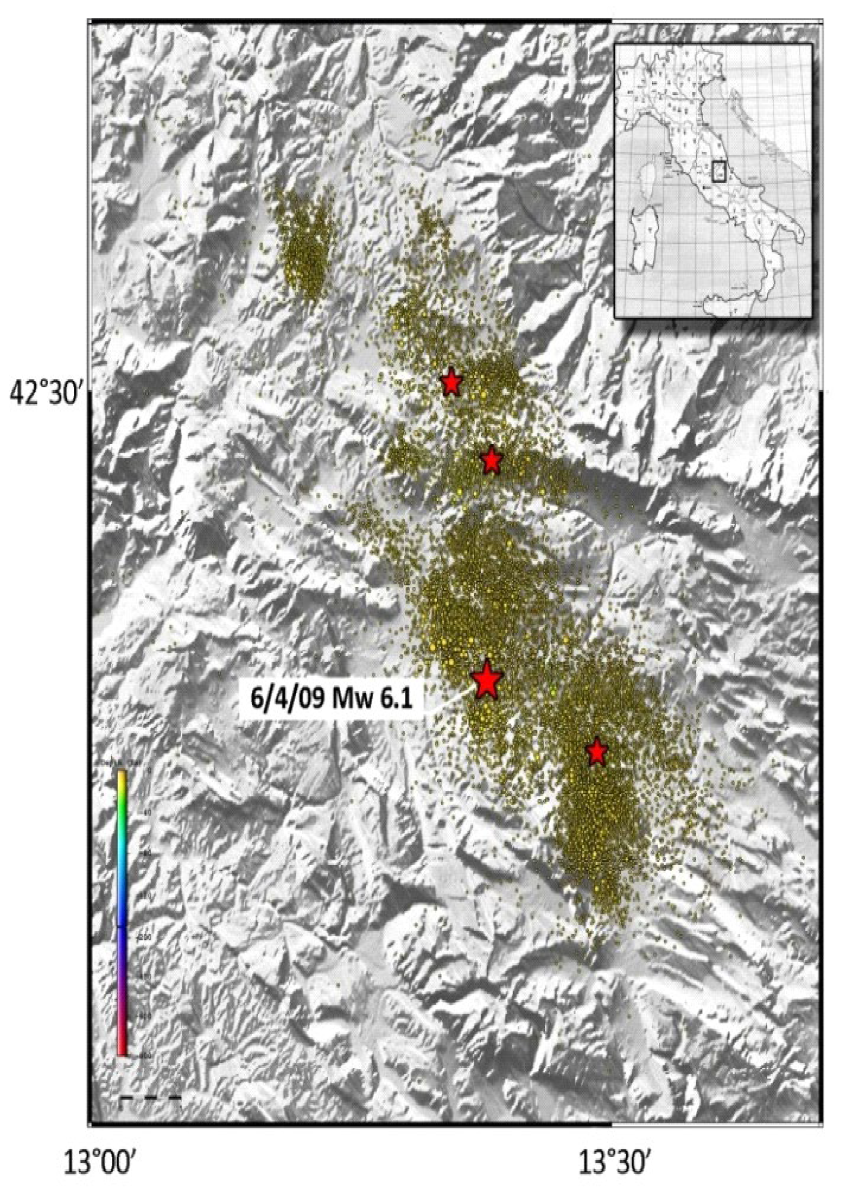
Figure 1.
Spatial distribution of the earthquakes in the L’Aquila area from 17 January to 25 July 2009. The earthquakes with Mw ≥ 5.0 are marked out with a star.
Figure 1.
Spatial distribution of the earthquakes in the L’Aquila area from 17 January to 25 July 2009. The earthquakes with Mw ≥ 5.0 are marked out with a star.

Figure 2.
Frequency–magnitude distribution and G–R law fitting calculated on 5 April 2009.

Figure 3.
Temporal variation of the b-value from 17 January to 25 July 2009. During the aftershock sequence, the number of events per day exceeded the 100-events threshold specified by the method for the determination of the b-value, and therefore only an average value (blue line) is shown. The vertical bars identify the days on which the highest magnitude earthquakes included in the analysis occurred.

Figure 4.
Temporal variation of the b-value from 15 to 25 July 2009. The black bar identifies the highest moment magnitude (4.4 Mw) earthquake recorded.
Figure 4.
Temporal variation of the b-value from 15 to 25 July 2009. The black bar identifies the highest moment magnitude (4.4 Mw) earthquake recorded.

Figure 5.
Spatial distribution of the earthquakes in the Emilia region from 1 March 1988 to 25 May 2013. The earthquakes with Mw ≥ 5.0 are marked out with a star.
Figure 5.
Spatial distribution of the earthquakes in the Emilia region from 1 March 1988 to 25 May 2013. The earthquakes with Mw ≥ 5.0 are marked out with a star.

Figure 6.
Temporal variation of the b-value from 1 March 1988 to 25 May 2013. During the aftershock sequence, the number of events per day exceeded the 25-event threshold specified by the method for the determination of the b-value, and therefore only the average value (blue line) is shown. The vertical bars identify the days on which the highest magnitude earthquakes included in the analysis occurred.

Figure 7.
Frequency-magnitude distribution and G–R law fitting calculated on 19 May 2012.

Figure 8.
Temporal variation of the b-value on 3 June 2012. The black bar identifies the highest moment magnitude (4.7 Mw) aftershock recorded.
Figure 8.
Temporal variation of the b-value on 3 June 2012. The black bar identifies the highest moment magnitude (4.7 Mw) aftershock recorded.

Figure 9.
Spatial distribution of the earthquakes in the Amatrice–Norcia area from 1 August to 30 November 2016. The earthquakes with Mw ≥ 5.0 are marked out with a star.
Figure 9.
Spatial distribution of the earthquakes in the Amatrice–Norcia area from 1 August to 30 November 2016. The earthquakes with Mw ≥ 5.0 are marked out with a star.

Figure 10.
Temporal variation of the b-value from 1 August to 30 November 2016. During the aftershock sequence, the number of events per day exceeded the 100-event threshold specified by the method for the determination of the b-value, and therefore only an average value (blue line) is shown. The vertical bars identify the days on which the highest magnitude earthquakes included in the analysis occurred.

Figure 11.
Frequency–magnitude distribution and G–R law fitting calculated on 23 August 2016.

Figure 12.
Temporal variation of the b-value on 30 October 2016. The black bar identifies the highest moment magnitude (6.5 Mw) aftershock recorded.
Figure 12.
Temporal variation of the b-value on 30 October 2016. The black bar identifies the highest moment magnitude (6.5 Mw) aftershock recorded.


Table 1.
List of main earthquakes for the seismic sequences of L’Aquila, the Emilia region, and Amatrice–Norcia.
Table 1.
List of main earthquakes for the seismic sequences of L’Aquila, the Emilia region, and Amatrice–Norcia.
| The L’Aquila Earthquakes | ||||
|---|---|---|---|---|
| Date | Magnitude | Magnitude type | Latitude–Longitude | Depth (km) |
| 6 April 2009 | 6.1 | Mw | 42.34–13.38° | 8 |
| 22 June 2009 | 4.4 | Mw | 42.45–13.35° | 14 |
| The Emilia Earthquakes | ||||
| 20 May 2012 | 5.8 | Mw | 44.90–11.26° | 10 |
| 3 June 2012 | 4.7 | Mw | 44.89–10.95° | 9 |
| The Amatrice–Norcia Earthquakes | ||||
| 24 August 2016 | 6.0 | Mw | 42.70–13.23° | 8 |
| 26 October 2016 | 5.9 | Mw | 42.91–13.09° | 10 |
| 30 October 2016 | 6.5 | Mw | 42.83–13.11° | 10 |
Disclaimer/Publisher’s Note: The statements, opinions and data contained in all publications are solely those of the individual author(s) and contributor(s) and not of MDPI and/or the editor(s). MDPI and/or the editor(s) disclaim responsibility for any injury to people or property resulting from any ideas, methods, instructions or products referred to in the content. |
© 2023 by the authors. Licensee MDPI, Basel, Switzerland. This article is an open access article distributed under the terms and conditions of the Creative Commons Attribution (CC BY) license (https://creativecommons.org/licenses/by/4.0/).
Share and Cite
MDPI and ACS Style
Lacidogna, G.; Borla, O.; De Marchi, V. Statistical Seismic Analysis by b-Value and Occurrence Time of the Latest Earthquakes in Italy. Remote Sens. 2023, 15, 5236. https://doi.org/10.3390/rs15215236
AMA Style
Lacidogna G, Borla O, De Marchi V. Statistical Seismic Analysis by b-Value and Occurrence Time of the Latest Earthquakes in Italy. Remote Sensing. 2023; 15(21):5236. https://doi.org/10.3390/rs15215236
Chicago/Turabian StyleLacidogna, Giuseppe, Oscar Borla, and Valentina De Marchi. 2023. "Statistical Seismic Analysis by b-Value and Occurrence Time of the Latest Earthquakes in Italy" Remote Sensing 15, no. 21: 5236. https://doi.org/10.3390/rs15215236
Note that from the first issue of 2016, this journal uses article numbers instead of page numbers. See further details here.