1. Introduction
Hydrogeological instability affects most of those areas characterized by geological and geomorphological fragility. When the phenomena affect densely populated zones, such as those found in most of Italy, the problem of safety becomes significant.
Rockfall is a phenomenon of natural instability due to the geodynamic activity ongoing on steep slopes. Triggering causes can be both natural processes such as precipitation, earthquakes, seismic shaking, or by gradual fall and human activities such as blasting, increased grazing, and machinery vibration [
1].
The phenomenon of rockfall occurs mainly in mountainous areas [
2] periodically affected by this kind of instability [
3].
Rock block rolling (weighing from a few kilograms to tens of tons) causes significant damage to underlying structures and infrastructures, often resulting in loss of life [
4]. Given that about one-tenth of the population lives in mountainous regions, it is self-evident that in such contexts the rockfall phenomenon is an important risk factor for the territory and the population [
5]. Thus, putting in place procedures for a hydrogeological risk assessment and analysis is a priority, aimed at risk mitigation actions to reduce the probability of natural disasters [
6].
Actions to mitigate rockfall risk consist of either anthropic interventions, such as the installation of catch fences or containment barriers and nets [
7], or natural factors such as the action of vegetation in stopping and/or slowing down rockfall phenomena.
The former are active actions that are costly both in realization and upkeep as they are subject to wearing and deterioration over time. In contrast, those natural origin actions do have low maintenance costs and therefore represent a more viable and sustainable protection action than the former [
8].
An example of such natural actions are the “protective forests”, whose action varies depending on the presence and type of plant root systems, which become part of the system of counteracting forces [
9,
10]. The active forces are represented by the tangential components with respect to the potential sliding plane of the moving rocks masses, which in turn are influenced by other elements such as rock mass, soil moisture, and biomass [
11].
Over time, the presence of forests and woodlands has ensured the presence of settlements along most of the valleys as they are a protective factor against phenomena such as avalanches, landslides, debris flows, and rockfalls. They also help to mitigate climate change, improve air quality and water management, prevent erosion, and also ensure better anchoring of surface soil [
12] as each plant coenosis results in increased internal cohesion in the surrounding soil layers [
13]. The effectiveness of the protective action is also influenced by the morphology of the soil, as a sharply steep slope contributes to a significant increase in the momentum of the rolling rock [
14].
Over the years, the scientific community has been increasingly interested in the rockfall phenomena, as evidenced by the review paper written by Bitar et al. [
15], which provides a report of scientific papers published from 1975 to 2019 on the topic. The review highlights the rapid increase in the number of papers in the last three year period analyzed, also highlighting the increasing use of remote sensing techniques. Indeed, hazard monitoring and early warning systems should certainly be improved by taking into consideration state-of-the-art methodologies and techniques, given that traditional methods (e.g., field surveys, literature reviews, cartographic interpretation, etc.) are not suitable for effective analyses due to long acquisition and processing times that frequently give back lag dates, in addition to high costs [
16]. Vice versa, remote sensing is an efficient technique for land monitoring and risk management, allowing the monitoring of protective forest to mitigate the risk of rockfall through systematic measurements at different scales, continuously, in real time and with the possibility of constructing databases backdated up to several decades [
17].
Over the last decade, significant progress has been made in terms of remote sensing data availability, classification methodologies, and expertise. A number of studies have been conducted, in particular on mapping based on UAV (Unmanned Aerial Vehicle) surveys [
18], 3D models from high-resolution LiDAR (Light Detection And Ranging) for detachment site identification [
19], and hazard mitigation through the use of TLS (Terrestrial Laser Scanner) monitoring [
20].
There is also evidence of the increasing use of an integrated approach, combining, for example, LiDAR and mapping data in a GIS environment to create a three-dimensional numerical model and to analyze the spatio-temporal characteristics of rockfall hazards [
21]. Today’s challenges involve the homogenization and management of such a large amount of data that needs the integration and support of automated image preprocessing and classification approaches [
22].
Analyses of vegetation are also important for monitoring water content and plant physiology, which indirectly gives an idea of the health of the biomass in terms of robustness and vigor. High-resolution images from satellite platforms are found to be effective in accurately rendering the vegetation cover of a protective forest [
23].
The applications of Machine Learning (ML) in the field of geosciences are many, and the use of these techniques is now growing rapidly given the increasing computational capabilities of computers and the accuracies achieved by the models [
24].
Some recent studies used ML models to estimate the probability of rockfall occurring using LiDAR data and taking into account other kinematic parameters that characterize rockfall kinematics [
25]. The results obtained could support the design and layout of protective barriers, suggest different mitigation processes, and improve urban planning strategies. Fanos et al. [
26] proposed a hybrid model based on machine learning for a rockfall source area in the presence of other landslide types. In addition to some morphometric parameters derived from LiDAR, they use both vegetation density maps and land use maps derived from satellite imagery. The model is found to be accurate and it proves that the conditioning factors derived from LiDAR can be used as an alternative to the geomechanical factors, such as discontinuity and fractures. Other studies also showed that the use of artificial intelligence techniques provides more accurate results for producing rockfall hazard maps [
27].
Nevertheless, the potential of processing satellite data with Artificial Intelligence (AI) techniques for the purpose of evaluating the protective action of forests in rockfall risk mitigation has not yet been widely exploited, as has the use of vegetation indices (VIs) within this integrated process.
By appropriately combining the spectral bands of the images, different VIs can be obtained, aimed at different analyses, for example, the Normalized Difference Vegetation Index (NDVI) and the Normalized Difference Water Index (NDWI). The NDVI is used to monitor changes in leaf area, such as changes in canopy structure (e.g., wilting or leaf drop) [
28], whereas the NDWI is used to monitor the canopy water content [
29], which contributes to biodiversity [
30] and affects ecosystem productivity [
31] and soil microbial communities [
32]. For more complex analyses, multiple VIs are often used. For example, Gu et al. [
33] proposes the monitoring of water stress in vegetation using both NDVI and NDWI.
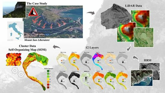
The aim of our work is to develop a methodology based on the integration of remotely sensed data, specifically optical satellite imagery and LiDAR data acquired from UAV, to identify the areas most prone to rockfall on a Test Case. The most resilient areas of the natural compartment in terms of health status, orientation age, robustness, and vigor will be identified using both morphometric parameters and VIs using the unsupervised ML method for classification. In these areas, it will be necessary to strengthen the contribution of the protection forest, supporting the artificial interventions (rockfall nets) already in place.
2. Case Study and Data Set
The case study analyzes the protective effect of the forest against natural hazards, such as rockfall, in the area of
Mount San Liberatore, located in Campania region (Italy) (
Figure 1).
The area is subject to frequent landslides and debris avalanches. When, as with the debris flows that affected the test site during a disastrous flood in October 1954, such collapses are triggered during the heavy rains by concomitant rock falls, they can be classified as complex landslides [
34,
35].
The Inventario dei Fenomeni Franosi in Italia (IFFI) “
https://www.progettoiffi.isprambiente.it/ (accessed on 1 July 2023)” aims to identify and map landslides on the Italian territory. Specifically, the information layer
Linear Landslides represents landslides whose length is much greater than the width and the latter is so small that it cannot be mapped at a scale of 1:25,000, while the information layer
Polygonal Landslides represents landslides smaller than 1 ha.
The test site is characterized by four landslide initiation points in the northwest part, from which three linear landslides and one polygonal landslide originate, inclusive of all debris flow types as reported in the IFFI inventory. The latter affected the underlying infrastructure.
The phenomena that occurred are characterized by extremely rapid movements with mostly granular soil transport. At present, all are in a quiescent state of activity.
The mountain sides facing the highway are characterized by an emergent rock substrate. The whole area, besides being subject to Debris Flow phenomena, is characterized by a high rockfall hazard. The exposed value is represented by a complex infrastructure network of viaducts, tunnels, and galleries along the northwestern slope of the mountain. The slope is partly covered by thick vegetation which limits the tumbling down speed of the rocks falling off.
In terms of ecology, the test site is a mixed deciduous and evergreen sclerophyll forest, as shown both in the
Carta della Natura “
https://www.isprambiente.gov.it/it/servizi/sistema-carta-della-natura (accessed on 1 July 2023)” and by in situ inspections. In botany, the dominant species influences the phytocoenosis of the forest. In our area,
Quercus ilex L., known as holm oak, is the dominant species which forms evergreen climax forests, having reached the final stage of its evolution, being made up of holm oak populations together with dry meadows, garrigue formations, and Mediterranean scrub.
Over time, the ecological role of this holm oak forest has been limited by strong human settlement which has resulted in its thinning on the coastal strip, whereas it still survives in steep, rocky areas, unpopulated, as in the test area. The holm oak is an evergreen Mediterranean sclerophyll, a long-lived, medium-sized tree with a dense canopy, especially when growing in rocky habitats. It is ideal for slope protection as its taproot system makes it resistant and stable, able to survive in extreme habitats such as rocky soils or vertical slopes. The taproot system gives the holm oak robustness, allowing it to penetrate soil up to several meters.
In addition to this dominant species, other vegetation covers are also present in the test site, listed below according to the typical three-layer forest structure: herbaceous, shrub, and tree. Herbaceous species include the Echium vulgare, Bituminaria bituminosa, and Antirrhinum tortuosum. This layer includes a perennial steppe grassland system dominated by Ampelodesmos mauritanicus, which represents one of the final stages of degradation of the ilex. Shrub species here include both those typical of thermophilic garrigue such as Rosmarinus officinalis and Cistus creticus, and formations that originate from the degradation of the ilex forest such as Viburnum tinus, Pistacia lentiscus, and Arbutus unedo. Last, the arboreal layer is made up of mixed coppice, i.e., broadleaf trees such as holm oak and downy oak (Quercus pubescens), Ostrya carpinifolia and Fraxinus ornus, mixed with conifers such as Pinus halepensis, Ostrya carpinifolia, and Fraxinus ornus.
Such a heterogeneous vegetation canopy enhances the protective effect of forests in the mitigation of rockfall hazard, as many different types of root systems contribute to the stabilization of the slope: deep roots confer stability, branched roots increase strength by hindering runoff, and lateral roots improve soil anchorage.
In the test site there is a mixed root network, composed of species with deeper taproots, such as those of the arbutus and holm oak, characterized by a central taproot that reaches up to 10 m deep, with nearby species with strong lateral roots, such as those of the downy oak, useful for stabilizing the surface layers of the soil. Lateral roots also serve to thicken the root network and enhance soil texture, such as those of the bay laurel, characterized by a vigorous rhizomatous-fasciculate root, rich in secondary roots continuously renewed from the base of the stem.
The LiDAR point cloud was acquired in June 2021 by a UAV, a quadricopter with a Velodyne Puck VLP-16 sensor (100 m measurement range and range accuracy up to 3 cm). The average density of the point cloud is about 500 points/m
2. The point cloud was edited to remove vegetation and artifacts using Cloud Compare software “
https://www.danielgm.net/cc/ (accessed on 1 June 2023)”. Given the presence of thick canopy vegetation and the peculiar morphological configuration of the site, to facilitate the extraction of points belonging to the bare ground, manual editing was carried out on sections of the cloud about 5 m wide, sliced parallel to the line of maximum slope.
To also have data on the area south of the Mount close to the highway where flying was not possible (area contoured in red,
Figure 1b), the point cloud was integrated with LiDAR data from the Ministry of the Environment and Protection of Land and Sea (MATTM), available on the Ministry’s website “
http://www.pcn.minambiente.it/mattm/progetto-pst-dati-lidar/ (accessed on 1 June 2023)”, having a density of about 2 pts/m
2.
Lidar data from the MATTM are released in different formats. Data in the *.xyz format used in our study are the geographic coordinates longitude and latitude, the elevation, the reflectance value, and a code that defines whether the point belongs to the terrain (2, “ground” point) or not (1, “no ground” point). Only points with code 2 were extracted.
The coordinates are given in the geodetic reference system WGS84 (EPSG:4979). In order to unify the reference systems and have all LiDAR data in the geodetic coordinate system used in Italy, that is RDN2008/UTM33 (EPSG: 7792), the transformations were made using grids provided by the
Istituto Geografico Militare [
36]. To merge the point clouds, a Bundle adjustment was made using Cloud Compare software. The integrated point cloud was resampled to 10 pts/m
2.
To analyze the vegetation health status through some vegetation indices, a Plèiades-HR 1B satellite image was used, having four spectral bands (blue, green, red, and NIR). The image was acquired on 30 June 2020, at 10:01 am, in the absence of cloud cover, covering an area of about 263 km2.
Image georeferencing was made with PCI Geomatica software using the Rational Polynomial Functions method (RPF) with the Rational Polynomial Coefficients (RPCs) provided with the image.
3. Methods
The methodology developed is based on the data integration acquired with remote sensing techniques, in particular high-resolution optical satellite images from the Plèiades HR-1B mission and LiDAR data acquired from UAV, integrated with MATTM data. The LiDAR data are used for the morphological description of the territory and the calculation of the average height of vegetation, while the satellite images are used to perform multispectral analyses and for the calculation of the VIs.
The workflow (
Figure 2) is based on the following main steps:
building the Digital Terrain Model (DTM) starting from the integrated LiDAR point cloud;
calculation of Digital Height Model (DHM);
calculation of morphometric parameters (DTM derived);
calculation of VIs from satellite images;
classification by Self-Organizing Map (SOM);
clustering with dendrogram analysis.
3.1. Vegetation Height and DTM-Derived Morphometric Parameters
Then, the DHM was produced by calculating the difference between the DSM and the DTM. The output is a raster with a resolution of 2 m, used to have an estimate of the average height of vegetation pixel by pixel.
The morphometric parameters considered most relevant for describing the landform of the test site slope were calculated from the DTM. More precisely, eight parameters [
37] were calculated: 1. Difference of curvature (Difc), 2. Slope insolation (Slins), 3. Rotor (Rot), 4. Aspect (Asp), 5. Cross-sectional curvature (Crosc), 6. Extreme curvature (Extc), 7. Vertical curvature (Verc), 8. Unsphericity curvature (Unsph).
Most of the named parameters are derived from the combination of different types of curvature, curvature being the parameter that best describes the land morphology and its surface change [
38]. In the relevant literature, there is some evidence that quadratic models can be used to describe geomorphometric features (ridges, slopes, valleys) and basic hill units [
39]. Higher-order polynomial models, which produce a non-uniform curvature for the analysis window, can represent specific land features with a more complex structure.
The morphometric parameter equations used in this work are those reported from Foroutan in [
40], shown in
Table 1. The partial derivatives of the DTM elevation values of the first-order (p, q), second-order (r, s, t) and third-order (a, b, c, d) have been calculated by Florinsky via a third-order polynomial [
41]. The method he developed for calculating the derivatives has proven to be more accurate in terms of Root Mean Square Error (RMSE), reducing the uncertainty in the computation of the morphometric parameters; thus, the derived maps result to be more detailed in the description of the features (shapes) of the land. The coefficients of the polynomial equation were computed using a 5 × 5 moving window on the DTM.
3.2. Vegetation Indices
In terms of electromagnetic spectrum, the reflectance pattern of the vegetation depends largely on leaf structure, pigment type, and water content [
42]. In general, healthy vegetation absorbs in the blue and red regions and reflects in the NIR and green, while stressed or senescent vegetation produces less chlorophyll, resulting in lower absorption values at the red and green wavelengths, and higher values at the NIR wavelength.
Specifically, chlorophyll absorbs in the blue and red, peaking around 0.67 μm and reflects in the green while leaf structure reflects mostly in the NIR in the range of 0.70 to 1.35 μm. This last band is relevant because it provides information about the mesophyll related to the phenological stage and developmental stages. Lastly, the water has a spectral response that is inversely proportional to that of healthy vegetation as it absorbs predominantly in the infrared.
As for the test site, of mixed conifers and deciduous forest, the spectral curves of the different species are slightly different from each other: conifers such as pine reflect more in the NIR, compared with broadleaf trees such as holm oak, downy oak, and arbutus which generally absorb more solar energy and present lower reflectance values than conifers, along the entire electromagnetic spectrum [
43].
To characterize the health status of the natural habitats of our area, three vegetation indices were calculated with a QGIS raster calculator “
https://www.qgis.org/it/site/ (accessed on 1 June 2023)”, using the spectral bands of the optical satellite image. The calculation equations are listed in
Table 2.
The first calculated index, NDVI, is used to monitor biomass and water content [
44] as it is sensitive to changes in chlorophyll content and intracellular spaces in the spongy mesophyll of leaves. NDVI allows an indirect assessment of vegetation health by estimating the photosynthetically active radiation absorbed [
45], but it is also used to estimate other characteristics such as leaf area index, plant biomass, and water presence [
46].
The values of the index can vary between −1 and 1; those between −1 and 0 are typical of uncultivated areas such as streams and anthropic areas. Positive values indicate greater vigor and photosynthetic activity, whereas negative values indicate vegetative stress with a consequent reduction in chlorophyll content and changes in internal leaf structure due to wilting. To calculate the index, the red and near-infrared spectral bands are used, which correspond, respectively, to the spectral region where there are peaks in the leaf pigment absorption, particularly chlorophyll, but also carotenoids, xanthophylls, and anthocyanins (red), and to the spectral region where greater leaf reflectance is present (NIR) [
47].
Although this index is commonly used in monitoring vegetation, it also has its drawbacks, such as saturation in the presence of biomass-rich areas where vigor is more evidenced by EVI [
48].
In addition, the index has a poor capacity to estimate the
Vegetation Water Content (VWC) [
49]. Despite the fact that NDVI is indeed a relevant parameter for monitoring natural productivity, it does not provide a direct measure of VWC since every species develops different mechanisms to resist water stress and some show signs of reduced evapotranspiration without experiencing a reduction in water content.
To overcome this limit, the NDWI, used to monitor the absorption of liquid water by vegetation, was calculated. There are several methods of calculating the index depending on the combination of bands used. The best performance, in terms of precision, accuracy, and spatial resolution, has been observed with the NDWI index combining the green and NIR bands [
50]. They correspond to the spectral bands in which the maximum reflectance of water and vegetation are observed, respectively.
In this work, the NDWI was calculated using McFeeters’ equation [
51]. Index values vary in the range of −1 to 1.
NDWI can be considered a complementary index to NDVI and not a substitute as it is less sensitive to atmospheric effects and the use of Green seems to be more effective not only for assessing water stress and predicting impacts related to the water content of the leaves, but also for monitoring the natural compartment as vegetation reflects these wavelengths, highlighting the reliability of the index for forest monitoring [
52]. The index also highlights liquid water content, especially in areas with few artifacts, because NIR is reflected less by water. Thus, positive values are observed in the presence of water, while vegetation and soil usually have zero or negative values [
53].
The last index calculated is EVI, which is used for monitoring photosynthetic activity because it has a greater sensitivity for monitoring canopies in areas of high biomass [
54]. It uses a mixture of reflectance estimates to allow a better monitoring of vegetation by decoupling the canopy background signal and reducing the atmospheric effect [
55].
To calculate EVI, in addition to the NIR and RED bands, the BLUE band is used. In particular, the BLUE band is used for the correction of the canopy background signals and also for a reduction in atmospheric influences, including aerosol scattering [
56].
EVI also improves linearity with biophysical parameters of vegetation, particularly with the
Leaf Area Index (LAI), which provides relevant information on the amount of photosynthesizing tissue per unit of soil surface area [
57], and is effective in monitoring vegetation, detecting changes, and assessing seasonal variations in evergreen forests [
58].
The range of values and their interpretation are similar to those of NDVI; particularly in the presence of vegetation, the index obtains values between 0.2 and 0.8.
3.3. Data Clustering Method Based on Self Organization Mapping (SOM)
Self-Organizing Maps or Kohonen’s map is a unsupervised neural network [
59]. The SOM algorithm comprises two different phases: the competitive phase and the cooperative phase. In the first phase, the neuron with the best matching, the “winner”, is chosen, and in the second phase, the weights of the winner and those of its lattice neighbors are updated. Only the minimum Euclidean distance variant of the SOM algorithm is considered. During the learning, not only the vector of the weights of the winner neuron is updated, but also those of its lattice neighbors, which react to similar input. This is realized using the neighborhood function, which is centered on the winning neuron and decreases as the lattice distance from it increases. The neurons of the map are connected to adjacent neurons by a neighborhood relation, which dictates the topology of the map. In our case, hexagonal neurons were used; therefore, each neuron has six neighboring neurons.
In this study, MATLAB R2020 “
https://www.mathworks.com (accessed on 1 May 2023)” was used as software application to apply the SOM algorithm to the data set provided since it has a built-in functionality for the SOM algorithm.
A 6 × 6 network with a total of 36 hexagonal neurons and a number of epochs equal to 1000 was used. A matrix with a number of rows equal to the number of layers (or predictors) used and a number of columns equal to the number of pixels of the raster is given as input. We have used the Batch training function in MATLAB (trainbu) where the weights are updated according to its learning function after each epoch. To estimate the network’s performance, we used the MSE function which measures according to the mean of squared errors.
As the input we gave twelve layers: the eight morphometric maps (1. Difc, 2. Slins, 3. Rot, 4. Asp, 5. Crosc, 6. Extc, 7. Verc, 8. Unsph), the map describing vegetation height (9. DHM), and the three maps describing its health condition (10. NDVI, 11. NDWI, 12. EVI).
The input values (the rows of the input matrix) were normalized to increase learning efficiency and ensure that input variables with wider ranges did not affect the computation of the Euclidean distance. At the end of the network training, a row vector with a number of columns equal to that of the input matrix will be provided as output. Each element of the vector will represent the index of the neuron associated with each individual column of the input matrix. This means that the same index will be associated with two columns of the input matrix that are deemed “similar”.
3.4. Dendrogram Analysis
The SOM will be made up of a number of clusters equal to the number of neurons set. To aggregate single clusters into sub-clusters with similar characteristics and, thus, reduce their number, we used Ward’s Agglomerative Hierarchical Clustering (AHC) method, implemented in MATLAB [
60]. In comparison with partitioning-based clustering algorithms such as K-means, AHC is more suitable for handling real-world data where finding a suitable set of parameters can be tricky [
61].
An AHC analysis using Ward’s method merges the two closest clusters into a sub-cluster based on the distance or dissimilarity index chosen. Ward’s method considers all possible cluster pairs and merges the two clusters that minimize the increment of total deviance from the centroid of the new sub-cluster. The Euclidean distance is used. Ward’s method aims to build small, homogeneous sub-clusters.
Once the proximity between objects in the data set has been computed, it is possible to determine how objects in the data set should be grouped into clusters, using the linkage function to define the distance between two clusters and links pairs of objects that are close together into binary clusters. The linkage function then links these newly formed clusters to each other and to other objects to create bigger clusters (sub-clusters) until all the objects in the original data set are linked together in a hierarchical tree.
The AHC can be visualized using a dendrogram that represents the relationships of similarity among a group of entities. It consists of many U-shaped lines that connect data points in a hierarchical tree and records the sequences of merges or splits [
62]. The height of each U represents the distance between the two data points being connected. The within-cluster sum of squares criterion was used to compute the optimal number of clusters; it is a measure of the variability of the observations within each cluster [
63].
The graph is constructed iteratively; the maximum number of iterations is set equal to the maximum number of sub-clusters and, at each iteration, the sum of the mean square deviations of each observation from the sub-cluster centroid is computed. In the first iteration, the number of sub-clusters (i) is set equal to 2, in subsequent iterations it is increased by one sub-cluster (i + 1). On the y-axis are shown the sum of the mean square deviations, on the x-axis, the corresponding number of sub-clusters. The optimal number of sub-clusters is found where an “elbow” appears in the graph. In general, a cluster that has a small sum of squares is more compact than a cluster with a large sum of squares.
4. Results
4.1. Morphometric Map and Vegetation Indices
The maps of the eight morphometric parameters cited in
Section 3.1, calculated on the DTM derived from the integrated LiDAR data, are shown in
Figure 3.
The Difc map, defined as the half-difference of the vertical and horizontal curvatures, shows which curve has more curvature; high values locate the preferential paths of rock rolling, i.e., all those channels that facilitate the transport of material downstream. In addition to the Difc map, two other maps provide similar information, plus they allow the channels to be wire-traced: these are the Extc map, which highlights ridge lines and thalweg lines more sharply, and the Unsph map, used to show the extent to which the shape of the surface is non-spherical at a given point.
The Slins map shows the amount of solar radiation received at a surface; it represents solar radiation power expressed in percent (from 0 to 100%) of the maximum possible that is reached for a solar ray direction perpendicular to the land surface. High values of Difc and low values of Slins identify steeply sloping channels, i.e., all those areas where a higher probability of material conveyance and the acceleration of rockfall due to steep slopes exist. This pattern is present in the northern and northwestern parts of the area and is almost totally lacking in the northeastern and southern parts.
The Rot map describes the trend of contour lines in planimetry by highlighting the changes in curvature. This parameter is especially useful in describing terrain roughness; compared to classic roughness indicators, the map has less noise in the case of high-resolution DTMs. As well, the Rot map highlights a marked difference between the highly morphologically articulated northern zone and the much smoother southern zone.
The Crosc map measures the curvature in the direction perpendicular to the line of maximum slope, high values characterize slopes with a higher probability of material detachment and rolling. The north and northwest side is characterized by high values alternating with low ones, in accordance with the other indicators that highlight the roughness of the terrain, in the areas where Asp values range between 200° and 260°.
The Verc map, defined as the curvature of a normal section of the land surface by a plane, including the gravity acceleration vector, identifies those areas where there are sudden changes in the ground profile that could produce the bounce and change of direction of a down-rolling rock. Areas having high values of Verc can, thus, represent critical zones to be watched when analyzing the roll rock dynamics. The Verc map of the test area highlights very clearly the stormwater drainage channels and the roads present in the western and northern side of the test area, as well as the foot of the vertical ridge to the north.
The DHM was classified using a green color palette with increasing gradient, directly proportional to the height of the vegetation above the ground (
Figure 3). Light green shades, closest to white, represent bare rock, hence the absence of vegetation. They describe mainly dirt trails and channels. Along the edges of these areas, there are brighter green tones, indicating the presence of bushy herbaceous species such as bituminous clover and red valerian, i.e., low Mediterranean scrub. Mid-green shades, which correspond to vegetation between three and ten m high, describe the shrub layer widely distributed in the test site and represented by vegetative species such as arbutus and laurel. Finally, the darker green shades describe the arboreal layer, i.e., the typical species of the Mediterranean forest characterized by large shrubs such as holm oak, downy oak, Aleppo pine, hornbeam, and manna ash. They are mostly present in the weakly sloping areas to the north and southeast.
To analyze the vegetation health status, three vegetation indices were calculated: NDVI, NDWI, and EVI, as detailed in
Section 3.2. The related maps are shown in
Figure 3.
The NDVI map shows large areas with rather high values between 0.8 and 0.6 (red to orange), indicating high vigorous vegetation. This result is in accordance with the trend of the phenological cycles of the main plant species in the test site as the period of satellite image acquisition, which is June 2020, coincides with flowering and/or the emission of new leaves.
Areas colored in yellow are those that have intermediate index values, between 0.5 and 0.3, that characterize mid vigorous vegetation. These are areas of complex morphology or near areas of accumulation or detachment. They can also be areas with poor vegetation cover, although very vigorous. Finally, areas colored in green are characterized by lower values, between 0.2 and 0, which are areas with almost no vegetation cover or bare soil. This typology is not very common in the test site; only small portions are observed to the north at the canals and to the west along the escarpment with marked steepness and at dirt trails.
The NDWI map displays mostly negative values showing a fair amount of drought, probably due to the even warm temperatures of the period in which the data were acquired; for June 2020, the average temperature was 24 °C. A low VWC could also be due to the low rainfall of the period considered as there were only three rainy days in May and four in June, with the last rainfall almost ten days away from the date of acquisition of the satellite image (30 September 2020). The presence of water bodies was not observed as the values ranged below 0.5 and also comprised even negative values, characteristic of NDWI in the case of vegetation presence. More precisely, the areas between −0.7 and −0.5 (in dark green) and those between −0.4 and −0.3 (in light green) correspond to high and medium vigorous vegetation cover, respectively. Those intermediate values between −0.2 and 0 (in yellow) represent areas with low vegetation, and finally, positive values between 0 and 0.04 (in orange and red) are observed at bare rock, as in the case of slope and/or in areas of rolling or accumulation.
With regard to the biomass estimation, given that the test area is densely vegetated, the EVI was calculated to optimize the results obtained from NDVI in order to better detail the level of vigor of the vegetative cover. For example, high values between 0.7 and 0.5 were observed in the northern zone.
Specifically, they characterize healthy vegetation. The highest values, between 0.7 and 0.6 (areas in red), are found in gently sloping areas, whereas values between 0.6 and 0.5 (in orange) are found in many other areas in which both herbaceous and shrub and tree species are present, so there is no noticeable dependence on vegetation height.
The range between 0.4 and 0.3 (in yellow) corresponds to vegetation with a medium level of vigor, whereas areas in green shades present sparse vegetation. Finally, those in blue included in the lowest range correspond to dirt trails, i.e., bare soil and/or accumulation and deposition areas.
In conclusion, from the qualitative point of view, the following considerations can be made regarding the vegetation in the analyzed area:
In the northern area, we observed the highest level of vigor, referring to species ranging in height from a few meters (herbaceous species) to about 10 m (shrub and tree species). In particular, the former has higher values of NDVI and EVI, so they are in a better state of health. This is in agreement with the botanical peculiarities of the species present, such as the laurel tree, which flowers until late spring, or the arbutus, a very hardy cultivar that is well resistant to adversity [
64];
In the western area, we observed the greatest spatial variability, which, of course, influences the spectral response, as observed especially in the EVI maps, as that area is very varied: it goes from dirt trails, channels, and escarpments devoid of vegetation, to mixed deciduous and sclerophyll evergreen forest up to 20 m high. In this area, in fact, there are populations of holm oaks whose flowering period is from June to August. Downy oak [
65], which flowers and at the same time sprouts new leaves starting in May, as well as manna ash and black hornbeam. The latter, precisely in the period of the satellite image under study, presents its peculiar infructescence characterized by pendulous bunches;
In the southern area, we observed thinning of the forest; actually, intermediate vigor values are observed in correspondence with smaller plant heights. At the trail entrance, an area characterized by a good level of vigor is present corresponding to plants that stand up to 15 m high, mostly holm oak, as confirmed by in situ visual inspection.
4.2. SOM Classification
The values of the pixels of the twelve calculated raster maps (layers) were normalized to the interval [0–1] and were organized into a matrix where the generic column represents the generic pixel to which the twelve values (twelve rows) related to the maps are associated. The number of clusters set during training can be seen in the UMap or UMatrix in
Figure 4, where the thirty-six purple hexagons represent the neurons and the red lines represent the connections between them. The color of the region in which the red line falls indicates the distance between the neurons joined by that line. Darker colors correspond to greater distance while lighter colors to shorter distance, as indicators of aggregation. In the map in
Figure 4, there are bands of dark colors separating neurons into clusters (light areas). The SOM network seems to have identified clusters, which are separated by the darker continuous regions.
To analyze each single contribution of the input layers in the training process, an analysis of the maps of weights associated with each input layer or feature becomes useful (
Figure 5). The weight assigned to the link between layer and neuron is represented by the color of the latter: darker colors mean higher weight. If the weight maps of two features are similar, it can be inferred that they are highly correlated, that is, they tend to con-tribute equally during the training phase.
Looking at the maps of the weights of the morphometric indices, it can be stated that the contribution made by each layer is different. There are no correlations between two different data sets. This aspect is in line with the results obtained by [
37], in which the feature selection (the maps) that maximized the prediction accuracy of the ML model was conducted by using the NCA classification algorithm.
As for the VIs weights maps, please note the correlation that exists between the EVI and NDVI. Both weights maps have similar chromaticity due to the fact that both indices are used to analyze the health status of vegetation, especially EVI is optimized for high canopy contexts. The NDVI and NDWI indices contribute differently, as is clearly evident from the corresponding weight maps.
We used Ward’s AHC Method to identify sub-clusters; the dendrogram is used to visualize the output (see
Section 3.3).
Figure 6a shows the “within-cluster sum of squares” plot, serving to identify the optimal number of sub-clusters, that is, the value located at the horizontal asymptotic trend of the curve (7 sub-clusters) [
66]. Assuming the number of sub-clusters to be seven, the cut-off threshold (320) within the dendrogram was found to derive the seven different cluster groups. The different colors of the branches of the dendrogram in
Figure 6b highlight the different neurons clustered in the sub-clusters.
4.3. Clusters Analysis
Figure 7 shows the map of the seven sub-clusters, each identifying regions with similar morphological and vegetation characteristics. With more detail:
sub-cluster 1, in dark green tones: identifies zones characterized by heterogeneous vegetation type (with predominance of tree species in the south and herbaceous species in the north), very vigorous (EVI values between 0.7 and 0.6), located at gently and regularized sloping;
sub-cluster 2, in medium tones of green: identifies mid-slope zones with mainly low vegetation (height up to 1.5 m), high vigor (EVI values between 0.7 and 0.6), located at stepped slopes;
sub-cluster 3, in light green: heterogeneous vegetation with mostly tree species (height between 5 and 10 m), high vigor (EVI values between 0.7 and 0.6), at mild slopes with rare rocky ledges;
sub-cluster 4, in yellow: identifies zones characterized by heterogeneous vegetation with a predominance of shrub species (height between 3 and 5 m), high vigor (EVI values between 0.6 and 0.5), at uneven moderate slopes and complex morphology;
sub-cluster 5, in orange: identifies zones characterized by heterogeneous species with shrub dominance (height between 1.5 and 3 m), medium vigor (EVI values between 0.5 and 0.4), corresponding to channels and discontinuities;
sub-cluster 6, in light red: identifies zones characterized mostly by herbaceous species, low vigor (EVI values between 0.4 and 0.3), at steep slopes and mostly close to rocky ridge;
sub-cluster 7, in dark red: identifies areas of outcrop rock and bare soil, mostly characterized by absence of vegetation at escarpments and rocky paths (EVI values less than 0.3).
Figure 7.
Classified map of the 7 sub-clusters, colored from green (1) to red (7), overlaid on Google Base-Map. Each sub-cluster represents an area having almost homogeneous characteristics in terms of morphology, vegetation vigor, and plant species. The characterization of the sub-clusters is shown in
Table 3.
Table 3 summarizes the morphological, vegetational characteristics and vigor values shown in
Figure 7. The last column gives a rating of protective forest contribution, labeled “+”, according to increasing values of protection (from 0 to 4). The greatest protection contribution (++++) is found in sub-cluster 3, which corresponds to an area covered by a high vigor tree layer along a regularized, non-complex morphology and gently sloping. Sub-clusters 1 and 4 follow, corresponding to areas with heterogeneous vegetation, which are assigned a high value of protective contribution (+++).
Among the two, sub-cluster 1, in particular, has a higher protective action in the south as there are taller and more robust trees, while in the north, the protection decreases as there is predominantly herbaceous layer. In sub-cluster 4, the value is greatly affected by morphological complexity. A medium protective contribution (++) is found in sub-cluster 2, where high vigor herbaceous vegetation prevails along medium gradient slopes, and in sub-cluster 5, where there is prevalence of intermediate vigor shrubs along irregular slopes characterized by discontinuity and channels.
Finally, the area where the protective contribution is the lowest (+) is in sub-cluster 6, where the vegetation is herbaceous, low vigor, and along high gradient slopes. No rating is given to sub-cluster 7 as the area is bare of vegetation.
Table 3.
Main characteristics of plant species, classified by sub-clusters (S-Cs).
Table 3.
Main characteristics of plant species, classified by sub-clusters (S-Cs).
| S-Cs | Morphology | Plant Species | Vigor | Protective
Capacity |
|---|
| 1 | Regularized gentle slopes | Heterogeneous species | Very High | +++ |
| 2 | Steep slopes, medium gradient | Mostly herbaceous species | Very High | ++ |
| 3 | Gently slopes w/rare rocky ledges | Heterogeneous species w/tree species dominance | Very High | ++++ |
| 4 | Irregular slopes, medium gradient, complex morphology | Heterogeneous species w/shrub dominance | High | +++ |
| 5 | Complex morphology featured by channels and discontinuities | Heterogeneous species w/shrub dominance | Medium | ++ |
| 6 | Rocky ridge, steep slopes | Herbaceous species | Low | + |
| 7 | Escarpments, dirt trails | Bare soil and outcrop rocks, vegetation absence | - | - |
5. Discussions
The contribution to rock retention associated with each individual sub-cluster identified was interpreted on the basis of the morphology of the area and the vigor status of the vegetation.
To support the interpretation given, in order to more accurately quantify the level of protection associated with each individual sub-cluster, it would be useful to make a check using non-experimental information data by analyzing the phenomena really occurred and inventoried. To this end, some maps were created in GIS with the landslide phenomena that occurred on the test area so as to verify the possible direct correlation, for example, between the sub-cluster classified as an area characterized by intermediate/low retention and the areas where landslides and rockfalls occurred.
In addition, the Susceptibility, Hazard, and Landslide Risk maps were also considered to analyze the areas with higher probability of the natural event occurring and the potential damage that the rockfall event may inflict on the structures/infrastructures present. This was conducted to assess whether the areas classified as protective forest, along with the artificial protections present, may in some way result in an improvement in terms of the mitigation of ground displacement phenomena, such as that of rockfall.
Figure 8 shows an excerpt of a selection of the maps contained in the
Piano Stralcio Assetto Idrogeologico “
Destra-Sele”, developed by the Southern Apennine District Basin Authority “
https://www.distrettoappenninomeridionale.it/ (accessed on 1 June 2023)”, with the landslide polygons from the IFFI project data set (inventory of landslide phenomena) elaborated by ISPRA (Istituto Superiore per la Ricerca e la Protezione Ambientale) “
https://www.progettoiffi.isprambiente.it (accessed on 1 June 2023)” overlaid, and the artificial protections (nets and rockfall barriers) identified in the area through in situ inspections and from UAV-based LiDAR data.
Looking at the figure, it can be inferred that:
most of the test area is exposed to high landslide hazard values (P4 and P3) and landslide risk (R3 and R4) wherein the high exposed value (D4) comes from the infrastructure present (A3, railway line, and SS18);
the test site was affected by debris flow phenomena that occurred in October 1954; the landslide inventory reports four landslide initiation points to the northwest, corresponding to four landslides (three linear and one polygonal), two of which caused damage to infrastructures. The debris flows were characterized by extremely rapid movements, carried mostly granular soil, and are currently in a quiescent state;
man-made protections are absent in the northern part of the test site, a rockfall protection gallery is present to the west, and a series of rockfall nets are present near the upper part of the ridge.
Figure 9 shows the sub-cluster map presented in
Section 4.3 with the Landslide Susceptibility map overlaid (by the Southern Apennine District’s Basin Authority) and the artificial protections present. Only areas with very high (S4) and high (S3) susceptibility values are analyzed and shown in the figure; a total of five polygons, named A through E, are obtained. A cross analysis was carried out to check the rockfalls that occurred within these polygons, the presence or absence of artificial protection elements, and the level of protection inferred from the sub-clusters. For better understanding, the results of the analyses have been reported in
Table 4. The maps in
Figure 8 and
Figure 9 were created in QGIS using the open source shape files provided by ISPRA and the Southern Apennine District Basin Authority.
In light of our analysis, the results obtained, and the comparisons made, we can safely say that in the field of monitoring and management of rockfall, it is crucial to put in place mitigation actions playing a joint effect of natural (such as protective forest) and artificial (such as nets and rockfall barriers) protection. Especially in the test area, the protective forest plays a key role in mitigating the risk of rockfall mainly in the areas of high landslide susceptibility (A–E) not adequately protected by artificial barriers as the vegetation interacts with the blocks in motion along the slope and slows their rolling speed downstream, mitigating their impact.
Especially the “B” and “C” polygons, which are located in areas where rocky material can transit, along irregular and discontinuous slopes, are interesting. More concretely, the protective contribution of the forest in these two polygons is referred to sub-clusters 3 and 4 for polygon “B”, and sub-clusters 4, 5 and 6 for polygon “C”, respectively.
These two polygons represent areas with widespread shrub vegetation and with good levels of vigor, affected by evident spatial variations, as observed from the Google Earth time series shown in
Figure 10. A loss of biomass can be noted in the time period from 2007 to 2017, which has completely receded in 2020. Therefore, these polygons could potentially increase their protective action if the natural phytocoenosis of the forest would be combined with the right silvicultural management and adequate monitoring.
6. Conclusions
In this paper, we described the methodology developed on a test area to classify the territory in terms of its susceptibility to the rockfall phenomenon. The remotely sensed data (LiDAR and Pleiades) were used as input to compute vegetation indices and morphometric parameters, which were subsequently integrated in an unsupervised Machine Learning process.
The derived products allowed us to identify macro-areas naturally most susceptible to hazard mitigation: this comparative analysis was later directed toward describing the characteristics of the various types of protective forest present. From the analysis of major events that have occurred in the past, a good correlation between the path of melt material and areas classified as having low susceptibility to retention was observed in our analyses.
The type of vegetation present and its state of health are not sufficient parameters to determine the potential for retention, as often happens when talking about protective forest. The study of the morphology of the area using specific morphometric parameters is crucial as it influences the trajectory of falling loose material. Therefore, integration with indicators of the vegetation health status is critical.
Furthermore, as found in our analyses that the calculation of such morphometric indicators, if conducted with the most accurate methodologies, can significantly improve the description of geomorphological forms by aiding classification processes.
The use of unsupervised ML techniques certainly produces more objective results than supervised techniques; the sole difficulty lies in the interpretation of the results, which will take on, even if to a small extent, a subjective bias.
A future possible development would be to compare the results achieved with those obtained from simulation analyses of rock retention made on the basis of numerical models available in the literature.


