1. Introduction
Radio occultation (RO) technology was initially developed to explore the vertical profile parameters of the ionospheres and atmospheres of the planets in the solar system [
1,
2]. Subsequently, Fishbach proposed using a global navigation satellite system (GNSS) RO to probe the atmospheric parameters of the Earth [
3]. The United States’ Global Positioning System (GPS) became more mature in the late 1980s, and GNSS RO began to develop gradually and flourish. Currently, mature GNSS RO utilizes established GNSS systems such as BDS, GPS, Galileo, and GLONASS as signal transmitters, with GNSS receivers mounted on low-Earth-orbit satellites (LEOs) as observation platforms. By receiving and analyzing signal delay caused by the bending of the signal path, atmospheric parameters such as refractive index, pressure, temperature, humidity, and other related products can be retrieved through inversion, which are of great significance in improving numerical weather models, monitoring climate change, and studying atmospheric dynamic processes [
4]. GNSS RO, with the capable of self-calibration and lack of bias, provides an effective complement to other data types, such as radiosondes and weather balloons [
5]. Therefore, GNSS RO products from LEOs are one of the most significant factors in reducing errors in numerical weather prediction models [
6]. If GNSS RO events are uniformly distributed globally, the greater the number of GNSS RO events is, the larger the volume of raw observational data available for inclusion in numerical weather prediction, leading to higher prediction precision [
5,
7]. To increase the number of GNSS RO events and improve the precision of numerical weather prediction, some GNSS RO missions have employed the strategy of increasing the number of receiving GNSS RO signal systems. For example, the COSMIC-2 and SPIRE missions receive occultation signals from the GPS, Galileo, and GLONASS systems (
https://data.cosmic.ucar.edu/gnss-ro/, accessed on 31 January 2022). The FengYun3 mission, starting from the FengYun3E (FY3E) satellite, receives occultation signals from the BDS, GPS, and Galileo systems.
China’s second-generation polar-orbiting meteorological satellite mission, known as FengYun3, has been launched to address the challenges of three-dimensional atmospheric probes, greatly enhance global data collection capability, and further improve remote sensing capabilities for cloud and surface features [
8]. The first FengYun3 satellite was launched in 2008 and six satellites have since been launched. As the fifth satellite, FY3E is the world’s first civil Sun-synchronous polar-orbiting orbit meteorological satellite. It operates at an orbital height of 836 km and has an inclination angle of 98.75 degrees, allowing it to perform GNSS RO measurements covering the global range of the Earth [
9]. FY3E was successfully launched on 5 July 2021, from the Jiuquan Satellite Launch Center in China using the Long March 4B carrier rocket. The remote sensing payload used for GNSS RO is called GNOS, which is unique in that it is the world’s first payload capable of simultaneously performing GNSS RO measurements for the GPS, BDS 2&3, and Galileo systems [
10]. Specifically, the FY3E occultation observation data are recorded in the ROEX format, which is an independent exchange format proposed by the National Space Science Center for easier GNSS RO data viewing and sharing. The ROEX format specifies the file type, composition structure, observed parameters, and data recording format of GNSS RO data. It is suitable for both independent exchange of space-based GNSS RO data and regional satellite navigation system GNSS RO data [
11].
Initially, the GNOS onboard FY3C and FY3D satellites received dual-frequency GPS and BDS-2 occultation signals. Subsequently, FY3E, FY3F, FY3G, and FY3H are capable of simultaneously receiving GNSS RO signals from GPS, BDS-2&3, and Galileo systems. It should be noted that, due to resource constraints, the reception was limited to dual-frequency RO signals from GPS and BDS systems, along with single-frequency RO signals from the Galileo system. Due to the difficulty in mitigating ionospheric effects with only single-frequency measurements, the conventional dual-frequency occultation process is not suitable for the Galileo single-frequency occultation process. Therefore, there is an urgent need to develop Galileo single-frequency occultation inversion algorithms. In previous experiments, researchers tested the GPS RO signals received by the Turborogue receiver on the Ørsted launched in February 1999. The results showed that compared to the dual-frequency occultation process, the accuracy of the single-frequency atmospheric occultation process was more affected by ionospheric effects and lower in precision above an altitude of 30 hPa. Montenbruck et al. used GPS L1 single-frequency amplitude and carrier phase observations for occultation inversion, which yielded slightly lower precision in refractive index products compared to dual-frequency occultation inversion [
12]. Larsen et al. reconstructed the second frequency using GPS L1 single-frequency pseudorange and carrier phase observations for a single-frequency occultation process on Ørsted. The refractive index products and dry temperature products showed relatively good precision compared to the European Centre for Medium-Range Weather Forecasts (ECMWFs) [
13]. However, Larsen et al. utilized the double differencing method for single-frequency occultation product inversion. While this approach reduces observation errors, it amplifies observation noise. Additionally, using a single differencing method or a zero-difference method for the GNSS RO process are both viable options. The single differencing method eliminates the receiver clock bias through differencing between the occultation-LEO link and the reference-LEO link. Since measurements from the reference satellite are single-frequency, eliminating ionospheric effects using the reference-LEO link will introduce pseudorange measurement noise. In the case of the zero-difference method, if the stability of the GNOS clock bias is high, it can improve the inversion precision of the zero-difference method and achieve similar inversion precision as the single differencing method [
14].
During the algorithm verification stage, we have already processed GPS single-frequency occultation data and BDS single-frequency occultation data from FY3E/GNOS, utilizing the single-frequency occultation process of reconstructing the second frequency with the zero-difference method. We have compared the processed products with the products derived from the dual-frequency occultation process and ERA5 reanalysis to assess their precision [
15,
16]. Compared with the dual-frequency occultation inversion, the correlation coefficient of the relative total electron content (relTEC) for single-frequency GPS and single-frequency BDS occultation inversion is greater than 0.95. The average deviation of the excess phase Doppler for single-frequency inversion is mostly less than 0.2%. The refractive index product obtained from single-frequency inversion has slightly lower precision compared to the dual-frequency inversion product, but they show good consistency in terms of deviation and root mean square (RMS) indicators compared to ERA5 reanalysis. This verifies the feasibility of the proposed method. In this study, actual FY3E Galileo single-frequency occultation observations were used for product inversion and precision analysis, with the aim of providing more occultation data for numerical weather prediction.
Section 2 of this paper describes the FY3E/GNOS Galileo E1 single-frequency occultation process method. In
Section 3, the global distribution of occultation events during the operational period of FY3E/GNOS is analyzed. Subsequent
Section 3.2 and
Section 3.3 evaluate the precision of the refractive index product and the dry temperature product inverted from the Galileo single-frequency occultation process.
Section 4 summarizes the research findings, and
Section 5 discusses the potential applications of the single-frequency occultation process.
2. Galileo E1 Single-Frequency Occultation Process Method
Figure 1 shows the Galileo E1 single-frequency occultation process flow, which includes the following steps:
FY3E/GNOS Level 0 data are segmented, converted into an appropriate format, and preprocessed to positioning observation data and occultation observation data.
FY3E precise orbit determination (POD) using FY3E positioning observation data and accurate GNSS products from IGS, resulting in precise position, velocity, and receiver clock bias.
Reconstruction of the carrier phase occultation observation data at the second frequency using pseudorange and carrier phase occultation observation data at Galileo E1 single-frequency.
Computation of the neutral atmosphere excess phase using the results from the previous three steps.
Inversion of the neutral atmosphere bending angle and refractive index using Abel integral transformation.
Retrieval of atmospheric temperature based on refractive index.
FY3E/GNOS includes two sets of positioning antennas, each with a corresponding RF unit, as well as two sets of atmospheric occultation antennas, each also equipped with an RF unit, in addition to a data processing unit. The antennas utilize low noise RF front end technology to ensure effective capture and processing of GNSS signals. The central frequencies of the receiver channels are shown in
Table 1. FY3E/GNOS simultaneously receives positioning signals and occultation signals: GPS L1&L2, BDS B1&B3, and Galileo E1 [
17]. The GNSS RO data record rule in GNOS is that when a rise or set GNSS RO event occurs, the carrier phase and amplitude of the radio signals are recorded at a high sampling rate of 50 Hz. The sampling rate in the pseudorange is recorded at a range of 1–50 Hz [
18].
Because Galileo positioning data have a single-frequency and Galileo positioning channels are significantly fewer than those of GPS, we utilize GPS L1&L2 positioning observation data for ground POD. The satellite position and velocity coordinates are all within the framework of the Earth-centered inertial coordinate system in the FY3E POD. FY3E is equipped with two positioning antennas, and the simplified dynamics method is employed by merging the observation data from the half field of view of the two antennas [
19]. The POD is computed at intervals of 30 s, and all GPS positioning observation data are processed in batches with a duration of 30 h. The fundamental observations used are ionosphere-free pseudorange and phase combinations. State vectors, including position, velocity, and clock bias, are estimated, along with empirical segment constants for acceleration (with 90 min intervals) and atmospheric drag (with 6-h intervals). The estimated results from each iteration are used as the initial orbit for the next iteration until the estimation residuals are sufficiently small.
In the radial-tangential-normal (RTN) reference coordinate system, POD achieves precision in position and velocity, using the RMS errors from overlapping arc segments as indicators.
Figure 2 illustrates the RMS errors for a 14-day FY3E POD analysis. Subfigure (A) represents the positional precision, which is lower than 2.5 cm along the T direction, and the average 3D RMS position precision is 1.91 cm. Subfigure (B) represents the velocity precision, which is lower than 25 μm/s along the R direction and, the average 3D RMS velocity precision is 15.96 μm/s. The computed position and velocity precision are sufficient for the inversion of atmospheric occultation products.
2.1. Reconstruct a Second Frequency Measurement
The previous section provided an overview of the characteristics of GNOS Galileo E1 occultation observation data and the FY3E POD. This section will discuss the reconstruction of the second frequency for the Galileo E1 single-frequency occultation process. Specifically, the reconstruction of the carrier phase measurement of the second frequency is based on the Galileo E1 single-frequency pseudorange measurement and carrier phase measurement . In theory, the choice of the second frequency is arbitrary, but for the versatility of the occultation Level 2 product process, the second frequency in this paper is based on the E5a in Galileo’s dual-frequency measurement, with a frequency of 1176.45 MHz.
The reconstructed occultation carrier phase measurement
is greatly affected by occultation pseudorange measurement noise. Therefore, a regularization method that minimizes the second derivative is commonly used to filter the noise in the occultation pseudorange measurements to reduce its impact on
[
20,
21,
22]. The first step is to construct a filtering matrix F. This is done by interpolating and patching the data gaps in
(sampled at a rate of 50 Hz) and
(sampled at a rate of 1–50 Hz) using a regularization parameter
, thereby reducing the noise influence from the observations. A value of
equal to
is chosen for a smoothing strength that corresponds to a low-pass filter with a cutoff frequency of approximately 0.05 Hz. To unify the sampling rates of
and
to 50 Hz, the size of the filtering matrix should be 500 × 500. Equation (1) represents the calculation formula for the filtering matrix F in the regularization method that minimizes the second derivative [
13]:
where
is a diagonal matrix, in which the corresponding diagonal elements are set to 1 at the positions where data exist in both
and
, and the remaining elements are set to 0. Its size is 500 × 500. The matrix
is a finite difference operator for the second derivative, which is represented by
as its transpose.
The second step is to calculate the reconstructed carrier phase measurements, denoted as
[
13].
As shown in Equation (2), the E5a frequency carrier phase measurement
is calculated by subtracting the carrier phase measurement
from the filtered
. Here,
represents the frequency of the Galileo E1 signal, and
represents the frequency of the Galileo E5a signal, both measured in Hz. Then, the term
can be used to invert the reconstructed relTEC of the second frequency, measured in total electron content units (TECUs). It has been statistically observed that the range of relTEC falls within 20 TECUs. The relTEC variation rate is involved in the excess phase Doppler calculation [
23]. Therefore,
Figure 3 illustrates the reconstructed relTEC variation rate for two representative occultation events, as shown in subplots (A) and (B). In particular, the calculation of the rate has nothing to do with the type of occultation rising or setting, and is based on the tangent point height from low to high. As can be seen from the figure, the relTEC variation rate is always positive, which indicates that relTEC is always increasing within 120 km.
2.2. Excess Phase Calculation
The initial purpose of reconstructing the second frequency is to adapt the Galileo E1 single-frequency occultation inversion algorithm to general GNSS occultation Level 2 inversion software (ROPP 6.0 is used in this paper).
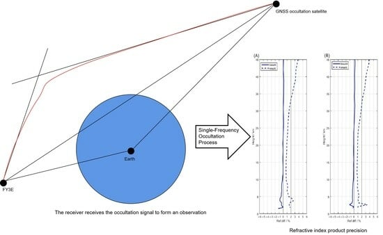
Figure 4 shows an illustration of a GNSS RO. FY3E (denoted by A) simultaneously receives signals from the GNSS satellite (denoted by B) undergoing an occultation event and signals from a high elevation angle GNSS satellite (denoted by C). The red path represents the bending of the signal in the atmosphere. In this case, AB represents the occultation-LEO link, and AC represents the reference-LEO link. In the single difference method, the AB observation equation is subtracted from the AC observation equation to eliminate the receiver clock bias. However, since the reference satellite C measurement is also a single frequency, the solution is affected by the noise in the reference satellite pseudorange measurement. Fortunately, the FY3E/GNOS clock has stability reaching the order of 10
−12 in one second, and the clock drift precision is sufficient for calculating the excess phase with relatively high precision using the zero-difference method.
The calculation of the excess phase using the zero-difference method only involves link AB and does not include link AC. This is expressed in Equation (3):
In the equation, represents the time of GNOS signal reception. represents the frequency of either or . , , , and represent the excess phase, geometric distance AB, carrier phase observation of E1 or reconstructed carrier phase observation of E5a, and corresponding phase ambiguity correction, respectively. Their units are all meters. is the speed of light, taken as a constant value of 2.99792458 × 10⁸ m/s. For the time-related parameters, and represent the clock biases of satellites A and B, respectively; and represent the relativistic effects on the clock biases of satellites A and B, respectively; and represents the radio wave propagation time. represents the relativistic effects, excluding clock biases. All time-related parameters are expressed in units of seconds. Information regarding the positions, velocities, and clock biases is obtained through POD. Additionally, represents measurement noise.
The excess phase Doppler is the input for refractive index product inversion. Therefore, it is necessary to convert the excess phase into excess phase Doppler [
24]. The equation for calculating the excess phase Doppler corresponding to the E1 and E5a frequencies is as follows:
The equation above, where
represents the wavelength of frequency
, provides the excess phase Doppler calculated from the E1 frequency occultation data and the reconstructed excess phase Doppler calculated from the E5a frequency observation data.
Figure 5A,B illustrate two representative occultation events. The
x-axis represents the excess phase Doppler in Hz, while the
y-axis represents the height in km in the form of a logarithmic axis.
From the figures, during the initial stages of occultation, the excess phase Doppler is close to zero. As the height decreases, the excess Doppler delay undergoes significant changes. This is because when the ray’s tangent point crosses the ionosphere and upper troposphere, where the medium is relatively thin, the signal amplitude remains relatively constant, resulting in the excess phase Doppler being close to zero. However, as the ray descends through the atmosphere, the refractive index becomes stronger, causing the ray to bend more, thus leading to a noticeable change in the excess Doppler delay [
25].
2.3. Inversion of Refractive Index Product and Temperature Product
Figure 6 illustrates the geometric optical model of GNSS RO. Assuming atmospheric symmetry, the rays in the figure are restricted to the same plane.
and
represent unit vectors in the direction of signal transmission for satellites A and B, respectively. α indicates the bending angle of the occultation event.
and
denote the position and velocity of the satellite obtained from POD.
With the aid of the quantities illustrated in
Figure 6, the excess phase Doppler can be expressed as:
Thus, the above equation has only two unknowns,
and
. Using Snell’s law in a spherically symmetric medium, we have the following equation:
and
represent the refractive indices at the positions of the FY3E and GNSS satellites, respectively, and can be approximated as 1. Utilizing Equations (5) and (6), the bending angle
can be calculated as follows:
Eliminating the ionospheric influence is crucial in inverting atmospheric products. Due to the dispersive effects of the ionosphere, the bending angle profiles calculated using Galileo E1 and reconstructed E5a exhibit differences. It can be assumed that the first-order term of the ionospheric bending angle can be eliminated through a linear combination using Equation (8) and
represents the impact parameter:
In the upper atmosphere above 40 km, the bending angle is relatively small, and the received signal is lower than the receiver’s thermal noise level. Therefore, it is necessary to employ a statistical optimization method to further eliminate ionospheric errors [
26].
Figure 7 shows the bending angle profiles originally and optimized by statistical optimization method, which can effectively correct the scene of sharp changes in the bending angle of the original data. This is because that the statistical optimization method combines measurement and bending angle of models. The coefficients are statistically optimized based on the noise characteristics of the bending angles, extrapolating from reliable low-altitude data to unreliable high-altitude data. Additionally, it incorporates bending angle intervention obtained from the a priori climatological model in mass spectrometer and incoherent scatter (MSIS) data [
27,
28].
Under atmospheric symmetry, the atmospheric refractive index can be obtained through the Abel integral transform using Equation (9):
In the equation, the additional parameters represent the following:
represents the atmospheric refractive index,
corresponds to the impact parameter specific to the current occultation. Both the bending angle and refractive index can be directly assimilated into numerical weather prediction models. With the assistance of numerical weather prediction models as prior information on the atmospheric state, the refractive index can be further inverted into meteorological parameters such as temperature using Equation (10):
In the equation,
represents atmospheric pressure in units of hPa,
represents the absolute temperature of the atmosphere in Kelvin (K), and
represents water vapor pressure. The first term on the right side represents the contribution of dry air to the refractive index, while the second term represents the contribution of water vapor. By neglecting the influence of moisture in the atmosphere, we can obtain the dry temperature:
When inverting for single-frequency occultation products, the largest error comes from the delay caused by the radio signal passing through the ionosphere. In this paper, a reconstruction of the second frequency is performed to calculate the excess phase, which is then used to validate the data through excess phase Doppler. In the bending angle calculation, the error associated with the first-order term of the ionosphere is eliminated, and the upper atmospheric ionospheric error is mitigated with the assistance of climatological models. This approach enables the inversion of occultation products with higher precision.
4. Summary
The Galileo occultation signal reception of the GNOS payload designed for the Fengyun3 series E/F/G/H satellites is based on the E1 single frequency. In this study, the actual Galileo single-frequency RO data obtained from the FY3E/GNOS receiver are used for the single-frequency occultation process. In terms of the number of occultation observations, the Galileo atmospheric occultation events received by FY3E/GNOS are distributed globally, similar to BDS and GPS occultation observations. The distribution is uniform, and the quantity is stable, which effectively improves the output of FY3E/GNOS occultation products and provides more data sources for global numerical weather prediction.
This study evaluates the precision of the products inverted from Galileo single-frequency RO data. The refractive index product and dry temperature product show good precision in the altitude range of 5–30 km. However, at lower altitudes, there are influences from ground reflections and the presence of turbulence, laminar flow, and inhomogeneities, which result in slightly larger biases in the refractive index and dry temperature average deviation. In the upper atmosphere, the inversion products are affected by high-frequency ionospheric and residual pseudorange noise, leading to increased errors.
In summary, the actual Galileo E1 single-frequency occultation data received by GNOS are accurate. The inversion products of single-frequency Galileo occultation serve as a valuable supplement to the FY3 occultation products, thereby enhancing the quantity of global occultation products.
5. Discussion
The GNSS RO remote sensing payload GNOS carried on FY3E for measuring atmospheric occultation data has the unique feature of receiving occultation signals from the GPS, BDS, and Galileo constellations simultaneously. However, the Galileo occultation signals received by FY3E/GNOS are single frequency. This study demonstrates the precise refractive index product and dry temperature product, indicating the correctness of Galileo single-frequency GNSS RO data. Therefore, it can contribute to increasing the number of global occultation events for numerical weather prediction.
The precision of single-frequency occultation process products above 30 km is significantly affected by factors such as high-frequency ionospheric and pseudorange noise residuals. However, the single-frequency occultation process products in the range of 5–30 km possess a considerable level of reliability. In terms of numerical assimilation and related applications, it is recommended to decrease the weighting of single-frequency process products below 5 km and above 30 km. The single-frequency occultation process employed in this study is derived from the Ørsted satellite and has been successfully validated in the FY3E GPS and BDS single-frequency occultation processes. It has also been applied to Galileo’s single-frequency occultation process. It is believed that this method has the potential to be applied to single-frequency occultation processes in other satellite occultation missions to increase the number of available occultation events.
Not only for the single-frequency occultation process but also for the L2P band of the GPS dual-frequency occultation process, which exhibits poor tracking near the bottom of the atmosphere, the method of second frequency reconstruction introduced in this paper can be considered to eliminate ionospheric errors. This means that a single-frequency occultation process can to some extent enhance the number of occultation data sources for global numerical weather prediction, thereby improving its precision. If there is more support from GNSS RO inversion data for research on numerical weather prediction and global climate change, it will greatly enhance the application capabilities of meteorological services, regardless of whether these GNSS RO inversion products come from dual-frequency or single-frequency occultation data.

 ,
, 


