
Analysis of the Matchability of Reference Imagery for Aircraft Based on Regional Scene Perception

1
State Key Laboratory of Information Engineering in Surveying, Mapping and Remote Sensing, Wuhan University, Wuhan 430079, China
2
School of Surveying, Mapping and Geosciences, Liaoning Technical University, Fuxin 125105, China
*
Author to whom correspondence should be addressed.
Remote Sens. 2023, 15(17), 4353; https://doi.org/10.3390/rs15174353
Submission received: 22 August 2023
/
Revised: 31 August 2023
/
Accepted: 1 September 2023
/
Published: 4 September 2023
(This article belongs to the Special Issue Remote Sensing Satellites Calibration and Validation)
Abstract
:Scene matching plays a vital role in the visual positioning of aircraft. The position and orientation of aircraft can be determined by comparing acquired real-time imagery with reference imagery. To enhance precise scene matching during flight, it is imperative to conduct a comprehensive analysis of the reference imagery’s matchability beforehand. Conventional approaches to image matchability analysis rely heavily on features that are manually designed. However, these features are inadequate in terms of comprehensiveness, efficiency, and taking into account the scene matching process, ultimately leading to unsatisfactory results. This paper innovatively proposes a core approach to quantifying matchability by utilizing scene information from imagery. The first proposal for generating image matchability samples through a simulation of the matching process has been developed. The RSPNet network architecture is designed to effectively leverage regional scene perception in order to accurately predict the matchability of reference imagery. This network comprises two core modules: saliency analysis and uniqueness analysis. The attention mechanism employed by saliency analysis module extracts features at different levels and scales, guaranteeing an accurate and meticulous quantification of image saliency. The uniqueness analysis module quantifies image uniqueness by comparing neighborhood scene features. The proposed method is compared with traditional and deep learning methods for experiments based on simulated datasets, respectively. The results demonstrate that RSPNet exhibits significant advantages in terms of accuracy and reliability.
1. Introduction
Scene matching technique refers to the real-time matching of imagery captured by aircraft with pre-prepared reference imagery, providing precise positioning for high-accuracy autonomous navigation of the aircraft [1,2]. The utilization of scene matching in assisted navigation is widely applied in both military and civilian domains, particularly in the military sector where it serves as a dependable technological assurance for accurate weapon guidance. The emergence of various image matching operators in the field of vision has overcome the technical bottleneck that previously constrained scene matching algorithms [3,4,5], as shown in Figure 1. Currently, addressing the challenge of matchability analysis for reference imagery as a supportive technical measure is crucial [6].
Matchability analysis is the process of extracting multi-source feature parameters from images and establishing a mapping model between feature parameters and the matching probability. The matchability performance of the reference imagery directly determines the accuracy of aircraft positioning. Consequently, it is important to adhere to principles [6] such as prominent object features, abundant information content in the image regions, exceptional uniqueness, and fulfillment of size requisites when selecting scene matching reference imagery.
The classic methods for matchability analysis typically involve constructing mapping models using manually designed features. However, they often lack consideration for the scene matching process. Different design principles for features and threshold parameter settings can yield varying results in terms of matchable regions. Therefore, traditional methods suffer from poor generality, high computational complexity, and low efficiency, leading to subpar application performance.
As one of the most important foundational technologies in artificial intelligence, deep learning has gradually extended its reach to the field of image analysis in recent years. Its applications in image classification, object recognition, and detection have become increasingly widespread. Representing the matchability of imagery solely with local shallow features is challenging due to the complex nature of this region-based feature, which lacks specific morphological characteristics. Deep learning models, on the other hand, overcome the limitations of traditional matchability analysis algorithms by automatically learning complex and latent features in images through training neural networks. They exhibit stronger adaptability and generalization capabilities [7].
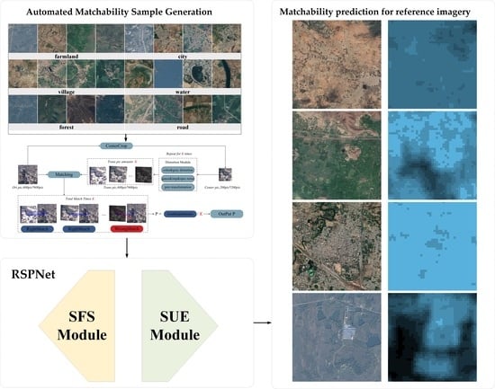
Currently, research on matchability analysis based on deep learning is relatively lacking. There are two main challenges in matchability analysis: (1) Lack of reliable open-source datasets. Deep learning techniques require a significant amount of specialized analysis and experimentation to support high-dimensional abstraction of matchability features in different scenarios. (2) Lack of feature extraction networks suitable for matchability analysis. Existing feature extraction networks lack research on the application scenarios and characteristics of matchability analysis. Unlike other feature extraction applications, matchable regions have low feature distinctiveness and an abundant amount of information in atypical structures that do not possess specific morphological characteristics, such as regions with obvious inflection points. Conventional neural networks (CNN) have low accuracy in feature extraction and selection, making it difficult to characterize and extract common features from matchable regions compared to highly discriminative and recognizable objects such as vehicles or ships. This paper proposes an innovative method for matchability analysis of reference imagery based on regional scene perception by using the scene information of the image to construct a sample simulation automatic generation scheme considering the matching process. This approach enables the automatic learning of image features and quantification of matchability levels, effectively minimizing manual intervention and reducing errors. It provides an important reference for aircraft route planning. The main contributions of this paper are below:
- An automated matchability sample generation method was constructed for image matchability analysis. In order to solve the lack of atypical structural sample features in multiple task scenarios, an automatic sample generation method that takes into account the matching process is designed using simulation technology.
- An image matchability analysis network, called RSPNet, based on region scene perception was proposed. This network takes into account the criterion of feature saliency and uniqueness in scene matching. The end-to-end matchability evaluation of reference imagery is realized through the analysis of scene-level feature perception.
- We conducted experiments on the WHU-SCENE-MATCHING dataset and compared our method with classical algorithms and deep learning methods. The results show that our method exhibits significant advantages compared to the other algorithms.
2. Related Works
2.1. Classical Methods
Classic matchability analysis methods are based on measuring the complexity of image information. They can generally be categorized into two types: hierarchical filtering-based and global analysis-based methods. The first type of method employs feature metrics to iteratively filter out regions that do not meet the threshold conditions based on template size, ultimately determining the final matchable region. However, it is important to note that this method may lead to the matchable region not being the best possible match for the entire image. The second method thoroughly evaluates all pixels in the image by utilizing feature evaluations. It accurately detects the region with the highest number of matchable points or the most effective matchable region. Despite its high computational cost, this method is capable of identifying the globally optimal matchable region. Overall, classic matchability analysis methods typically involve two steps: defining features and feature assessments [8].
Defining features refers to defining feature indicators that reflect the matchability performance of the input image by reducing the dimensionality of the data or restructuring its structure. In 1972, Johnson [9] first proposed the theory and method of selecting matchable regions. Since then, researchers have proposed using image descriptive feature parameters such as grayscale variance, edge density, number of independent pixels, information entropy, and self-repeating patterns to differentiate regions suitable for matching from those unsuitable for matching through hierarchical filtering [10,11,12,13]. Wei [14] proposed a matchability estimation method by establishing a correlation model between signal-to-noise ratio and matching accuracy. Giusti [15] used non-downsampling to extract local extrema points as interest points and filtered the matching region based on the amplitude and structural characteristics of the interest points. However, a single feature cannot reflect global characteristics, and this limitation can lead to significant errors in matching under certain circumstances. Therefore, multiple feature indicators need to be combined to comprehensively evaluate the performance of image matching. Yang [16] proposed a matchable region selection method based on pattern recognition, which selected six image features to construct an image feature descriptor and used support vector machines to establish a classification decision function for selecting matchable regions. However, this method requires calculating unique features for each candidate image, which is time-consuming. In addition, if new image categories need to be processed, it is necessary to remake training data and retrain the model. Zhang [17] proposed a method for selecting SAR matchable regions using a combination weighting method that combines four traditional feature indicators, including edge density, number of independent pixels, information entropy, and main-to-secondary peak ratio, as weights to achieve a more comprehensive and accurate selection of matchable regions.
Feature assessment refers to the process of selecting matchable regions based on threshold values of feature indicators. Xu et al. [18] first select different candidate regions and then evaluate these regions based on feature comparisons to obtain matchable regions. Cai [19] uses the Analytic Hierarchy Process to comprehensively evaluate the matchable regions and divide them into matchable and non-matchable regions. Luo [20] first calculates feature indicators for each pixel and then formulates a matchable region selection strategy based on the number of points exceeding the threshold and the distance interval in the matchable region. These methods employ various criteria and techniques to assess the suitability of regions for matching based on feature indicators. By comparing and evaluating these indicators, the methods determine the matchable regions and separate them from non-matchable regions. The selection strategies may vary depending on the specific thresholds and criteria applied in each method.
Indeed, the mentioned methods heavily rely on domain knowledge for statistical analysis of image grayscale values to design feature extractors, making the handcrafted features specific to certain scenarios. Furthermore, these methods only consider the requirements of matchable regions and overlook the demands of matching algorithms. However, matchability is often influenced by imaging conditions, and handcrafted features are not robust and general enough to adapt to real-time geometric distortion and color variations in images.
2.2. Matchability Analysis Based on Deep Learning
The field of image classification has been greatly impacted by deep learning, prompting several researchers to suggest matchability analysis methods utilizing deep learning models. With massive volumes of data, these methods imitate the feature representations of reference and target images in the matching process by leveraging the tremendous data fitting capabilities of CNN. By training the network, they obtain a mapping function that can assess the degree of matchability.
In the work by Wang [21], CNN features were first applied to matchability analysis of images. However, this method only considered the intrinsic features of the images and ignored the influence of the matching process on matchability, resulting in limited generalizability. Sun [22] proposed a method to generate a reference image sample library by simulating real-time images and then utilized a ResNet network for matchable region classification. Similarly, Yang Jiao [23] constructed a dataset using a similar approach and performed matchability regression analysis using both ResNet-50 and AlexNet.
The fixed receptive field of convolutional operations limits the integration of global features, making it challenging to describe the global information of features. ResNet [24,25,26] was proposed to address this issue and has been applied in various fields such as model mapping estimation, target area feature recognition, and land object segmentation. It further optimizes the ResNet architecture by introducing a multi-branch structure and improving the feature representation capability. In addition, the introduction and widespread use of Transformer [27] and self-attention mechanisms [28] have greatly improved the utilization of global information in images. By reallocating the weights of image feature extraction, these methods achieve multi-dimensional feature extraction capabilities for scene matching. Sun et al. [29] proposed an F3-Net network suitable for constructing the mapping relationship between unmanned aircraft scene images and reference imagery. The network leverages the self-attention mechanism and generates the probability distribution of features in the scene image based on semantic consistency. Similarly, the study by Arjovsky et al. [30] also achieved the probability distribution of high-level semantic features between scene images and reference imagery. By considering the global information and semantic coherence, these methods aim to enhance the matchability analysis and improve the accuracy and robustness of scene matching.
Directly applying feature extraction networks from the computer vision field to matchability analysis is challenging due to the unique evaluation criteria and requirements of the analysis. Currently, there is a shortage of deep learning techniques that are tailored for matchability analysis of reference imagery. To effectively analyze matchability of aircraft reference imagery based on region-level scene perception, it is crucial to design specialized network architectures. This design is intended to provide reliable information about the reference imagery for scene matching.
3. Network Architecture for Image Matchability Analysis Based on Regional Scene Perception
3.1. An Automated Matchability Sample Generation Methods
Most of the traditional matchability analysis methods are based on manually designed pixel-level shallow features, and statistical regression was used to achieve matchability modelling. These methods only consider the information in the image itself and lack consideration of the imaging process, resulting in unstable results, poor generality, and low efficiency. Deep learning automatically learns the features in the image by training neural networks, which can capture some complex and implicit features in the image. It is more adaptable and generalizable to complex problems. But the performance of deep learning models relies on a large amount of data training. There is a problem of missing training samples covering multiple task scenarios for the task of image matchability analysis. As matchable regions are atypical structures without specific morphological features, it is difficult to describe and extract common features, which brings great challenges to feature extraction and screening.
In this paper, we quantify the matchability with the matching probability index and design an automated sample production process for a matchability analysis task. The adaptive distortion model is employed to generate simulated real-time maps by imaging perturbation of the reference imagery. The number and probability of correctly matched real-time images is counted to calculate quantitative evaluation index of the matchability of the reference image. The strategy for aircraft image matching simulation encompasses two steps: perturbation and quantization, as illustrated in Figure 2.
(1) Perturbation: Simulated experiments necessitate considering the discrepancies between real-time and reference imagery and establishing an effective distortion perturbation model to ensure a closer resemblance of the simulated real-time image data to practical applications. The distortion model is derived from the disparities encountered in actual matching scenarios between the reference and real-time imagery and is influenced by the specific image characteristics employed. In this study’s simulated experiments, the predominant distortion model encompasses color and grayscale distortion models, noise interference models (such as Gaussian noise, salt-and-pepper noise, and speckle noise), as well as geometric distortion models (including projection transformations). Specifically, the noise addition ratio is set at 0.01, the projection transformation ratio at 0.1, and the ratios for brightness, color, and contrast transformations at 0.1. Random coefficients are introduced for each distortion occurrence. The simulated distortion demonstration is depicted in Figure 3.
(2) Quantization: The distortion model is used to generate simulated distorted images, which are then matched using standard matching algorithms to produce the simulated distorted images. By ensuring high accuracy in measuring flight altitude and attitude parameters, we can assume a straightforward translation transformation relationship between real-time and reference imagery. This allows for the use of a simple matching method. However, the inertial navigation system of the aircraft has lower accuracy and there are measurement errors in the attitude system in most cases. So, there may be scale and rotation changes between the real-time and reference imagery. In such cases, feature-based image matching methods are employed to improve matching accuracy. This study utilizes two commonly used point feature matching methods: SIFT-FLANN matching and AKAZE-BFM matching [31,32,33]. These methods are used to match the real-time images generated by the simulated distortion model with the reference imagery. The correctness of the match is determined by whether the distance deviation between the correct matching position and the actual matching position is less than a threshold value . When the number of iterations reaches the threshold value , the number of correct matches is denoted as , and the calculation formula is as follows:
where stands for practical matchability.
In the process of developing aircraft navigation systems, hang-flight experiments are considered to be the most precise and objective approach for obtaining match probabilities. However, these experiments are characterized by substantial time and financial expenditures. The sample labeling data are obtained by computing match probabilities through simulation experiments. The use of simulation experiments is advantageous due to its efficiency, reliability, cost-effectiveness, and the ability to be repeated multiple times within a controlled environment. Consequently, this study employs simulation methods to analyze the matching compatibility between reference and real-time imagery in order to mitigate costs and risks [34].
3.2. RSPNet
A targeted feature learning framework, called RSPNet, was proposed for the task of image matchability analysis in scene matching. Our method consists of two modules: a saliency module that considers multi-level feature adaptive fusion and a uniqueness module based on regional scene similarity evaluation [32,33]. The saliency module extracts saliency features based on regional scenes by stacking the residual U-Net’s feature pyramid module and applies channel attention to achieve multi-level and multi-scale fusion of region saliency features. The uniqueness evaluation module calculates the similarity of different regional scenes using a sliding window and combines the saliency and uniqueness of the features through summation. The two modules are connected by non-overlapping convolution layers. The specific structure is depicted in Figure 4.
3.2.1. Saliency Analysis Module
In the context of saliency analysis, routine semantic segmentation models often suffer from a loss of fine-grained spatial details and incomplete contextual information across different scales [34,35] due to the downsampling process during convolution and max pooling. This results in a failure to capture the high-resolution spatial features of the original image. To address the limitation and extract deeper structural information while preserving accurate local details, we draw inspiration from the channel attention mechanism [36]. Hence, we propose a novel saliency module, named the Self-Adaption Fusion Saliency Module (SFS), which incorporates multi-level feature adaptive fusion.
The SFS module allows for the acquisition of deep structural characteristics without compromising the precision of local features. Since the convolutional operation extracts representative information by mixing across channels, the SFS module is implemented to emphasize meaningful feature hierarchies on different hierarchical spatial axes. Thus, the implication of the SFS module is to effectively help information flow within the network by learning which information to emphasis or suppress.
Specifically, we first utilize Residual U-Blocks (RSU) [37,38] to extract multi-scale features at each level of the feature pyramid. These features are then aggregated and fed into the Multi-level Feature Adaptive Fusion module for adaptive weight allocation and fusion, resulting in a saliency feature map. As illustrated in Figure 5, RSU is an excellent module for image saliency analysis. It incorporates residual blocks into the U-Net architecture, comprising an encoder, a decoder, and cross-layer connections. The encoder utilizes residual blocks from ResNet to extract high-level feature representations, while the decoder employs the decoding structure of U-Net [39] to restore resolution and capture detailed information. The cross-layer connections are applied in the decoder, enabling it to leverage the feature information from the encoder for improved saliency analysis accuracy.
As shown in Figure 5, we stack RSU with decreasing encoder-decoder layers, namely 7, 6, 5, and 4, to extract multi-scale features. A downsampling layer is applied between every two consecutive layers. The output feature sizes of RSU are 600-300-150-75. The multi-scale features are then aggregated and fed into the Multi-Level Feature Adaptive Fusion module. In the fusion module, we first perform max pooling and average pooling along the channels for each input multi-level feature (i = 0, 1, 2, 3). The pooled feature size for is 1 × 1 × , where represents the number of channels. Next, the pooled features are aggregated, resulting in a channel size . We apply fully connected operations to the two aggregated features separately, compressing their channels to 4. Subsequently, we add the corresponding elements of the two resulting 2D vectors to obtain a vector containing channel weight information. Finally, we multiply element-wise with the input feature map , which is uniformly sampled to the size of 75, resulting in a feature map with channel weight information and multi-scale features.
3.2.2. Uniqueness Analysis Module
The uniqueness of the image indicates the degree of similarity between real-time image and the surrounding environment. When the regional scene is more different from the environment, the features obtained by the matching algorithm are unique, and thus the image and the scene are less prone to be mis-matched. On the contrary, the higher the degree of similarity between the regional scene and the environment, the more similar features are extracted, and the more likely it is to lead to mis-matching. For example, notable features include multiple corner points of the field that are too similar, resulting in a high susceptibility to mis-matching in a large area of agricultural land. In contrast, the characteristics of the village area are significantly different from the environment, such as buildings and other structural and textural features, so that a correct match can be achieved to serve the positioning and navigation tasks of the aircraft between the real-time image and reference imagery.
To address the concern of scene similarity in matchability analysis, this paper proposes the Saliency and Uniqueness Evaluation Module (SUE) based on region-level scene perception. This module takes saliency features as input and evaluates uniqueness based on the similarity of region features while considering environmental differences.
The SUE module is shown in Figure 6. The saliency feature map extracted by the previous module is passed through a non-overlapping convolutional layer with both a convolutional kernel and a step size of 25 to obtain a feature of size 3, which is used as an input to the SUE module [40]. The region is divided into a 3 × 3 grid using a sliding window approach, resulting in 3 × 3 regions with a size of 1 × 1 × C. Among them, represents the feature of the central region, while the other features represent the surrounding regions. On one hand, the feature vector of is correlated with the feature vectors of the surrounding sub-regions using the Euclidean distance as the evaluation criterion. The minimum Euclidean distance, denoted as , is considered as the global uniqueness output. A smaller Euclidean distance indicates higher similarity to the feature and lower uniqueness, while a larger Euclidean distance implies lower similarity and higher uniqueness. On the other hand, the feature is processed through a fully connected layer to output its saliency level, denoted as , in the scene. Finally, the uniqueness level and saliency level are fused using summation to obtain the matchability prediction value , which contains both saliency and uniqueness information.
3.2.3. Loss Function
In order to ensure the accuracy of matchability, Mean Absolute Error (MAE) was used to calculate Loss with the following formula.
where stands for image true matchability and stands for predicted matchability; where is calculated as follows, we use to maintain the learning balance between and .
4. Experiment and Analysis
4.1. Datasets
WHU-SCENE-MATCHING is a deep learning dataset specifically designed for matchability analysis of scenes. The dataset contains 40,000 optical images with a size of 600 pixels and a spatial resolution of 2 m. The dataset covers approximately 90,000 square kilometers of the region, including parts of India (E78-E84, N25-N20), western Tibet (E90-E93, N32-N29), and Eastern Hubei region (E113-E116, N31-N29), as shown in Figure 7.
The dataset covers a diverse range of climate types and includes different terrains and vegetation. The elevation ranges from 50m to 3000m. During the generation process, the original images were cropped, and subregions with a center-to-center distance of 600 were selected as the images. The main land cover types in the WHU-SCENE-MATCHING dataset are shown in Figure 8.
In our experiments, 80% of the WHU-SCENE-MATCHING dataset was used as the training set, while the remaining 20% was used as the test set. To avoid potential correlations between training and test samples, the training and test sets were divided into two separate regions.
This division ensures that the training set and test set contain independent and distinct regions, reducing the possibility of overfitting and providing a more reliable evaluation of the model’s performance on unseen data. By using separate regions, we can better assess the generalization ability of our proposed method and validate its effectiveness in matchability analysis.
4.2. Experimental Design
To validate the matchability analysis capability of our method on reference imagery, we conducted targeted experimental designs. Based on the WHU-SCENE-MATCHING dataset, we compared the proposed method with classical methods and deep learning methods as follows:
- Comparative experiment with classical method: Different methods as mentioned in [41], such as image variance, edge density, and phase correlation length were applied to analyze image matchability. Threshold parameters from related literature and extensive experimentation were used to determine correct matches, considering a matching error of less than 3 pixels.
- Comparative experiment with deep learning method: Different network architectures were adopted for comparison experiments as mentioned in [4,42,43], such as ResNet, DeepLabV3+, and AlexNet. To adapt to the matchability regression task in our paper, we made specific modifications to the model structure as in reference [23]. The number of fully connected layers was changed to 1. MAE was used as the loss function.
4.3. Parameter Settings
In the experiments, the SGD optimizer was applied to train the model. The hyperparameters were set as follows: the batch size was set to 8, the number of epochs was set to 300, the momentum value was set to 0.9, and the initial learning rate was set to 0.000001. The learning rate was adjusted using cosine annealing and the updated value was used to update the parameters.
4.4. Evaluation Indicators
In the classical method comparison experiment, the number of matchable regions and the average matchability probability are used as evaluation criteria to assess the effectiveness of different methods. For deep learning methods, common evaluation metrics for regression tasks such as MAE, Mean Squared Error (MSE), Root Mean Squared Error (RMSE), and were utilized to evaluate the performance of different network models. In addition, the receiver operation characteristics (ROC) statistical method was introduced to set valid values for predictions with a matchability rating threshold higher than 5 to be statistically analyzed to further assess the performance capability of the model.
Once the deep learning models were trained, they automatically extract matchability values from N test images. The true values, average true value, and predicted values are denoted as , , and , respectively. Regression metrics are then calculated to verify the accuracy of the model.
4.5. Experimental Results
4.5.1. Comparative Experiments with Conventional Methods
According to the comparative experimental design described in Section 5.1, we conducted a comparative experiment using the WHU-SCENE-MATCHING dataset with classical methods (based on image variance, edge density, and phase correlation length). Table 1 below presents the performance comparison results of our proposed method and the classical methods in matchability analysis.
The analysis of the results in Table 1 reveals that our proposed method demonstrates superior performance in terms of NMA and PMA compared with the classical methods. The number of matchable regions selected by our method is 607, which significantly outperforms the results obtained by the other methods. As for the average matchability probability of PMA, our method achieves a remarkable value of 0.9156. On the other hand, the PUA exhibit a lower average matchability probability of 0.4334, indicating a more accurate differentiation of matchable regions.
Among the classical methods, the image variance-based method shows promising results compared to the other two methods, with NMA count of 551 and an average matchability probability of 0.8182. However, the image variance-based method only considers the distribution of pixel values in the entire image, neglecting local image features and spatial structures according Figure 9. Consequently, it may introduce errors in matchability analysis, particularly in complex or spatially structured scenes where the filtering results are sensitive to variations.
The edge density-based method solely considers edge information while disregarding texture information, leading to potential errors when analyzing regions with rich textures. The phase correlation length-based method performs better at distinguishing boundaries between different objects due to its sensitivity to grayscale variations, but it exhibits subpar performance in other regions.
Overall, classical algorithms have limitations when it comes to adapting to different types of target objects in various scenes. The proposed RSPNet model in this study demonstrates enhanced versatility. It not only exhibits outstanding performance in filtering regions containing structural features, texture characteristics, and complex attributes, but also showcases higher precision in segmenting matchable regions. Moreover, our method has a distinctive exclusion effect that efficiently eliminates duplicated feature regions that may affect scene matching.
4.5.2. Comparative Experiments with Deep Learning Methods
Based on the comparative experiments designed in Section 5.1, various metrics including MAE, MSE, RMSE, and were used to evaluate the performance of different models on the WHU-SCENE-MATCHING dataset. Table 2 below presents the performance comparison results of our proposed method and other deep learning approaches in matchability analysis.
The experimental results indicate that our proposed method outperforms the ResNet, AlexNet, and DeepLabV3+ models in the task of matchability analysis. Specifically, our method achieves an average precision of 0.81, demonstrating a significant performance advantage over the other methods. In terms of stability, both MSE and RMSE achieve the best results among all the methods. Additionally, our method exhibits better interpretability, as the regression model can explain the dependent variable (with a larger ) from Figure 10d. Furthermore, our method has a shorter training time, making it more suitable for regression analysis of scene matchability.
To further evaluate the performance of the proposed model, we converted the regression task of matchability grading into a binary classification problem. We perform the statistical evaluation of the ROC of different models by setting the matching grade threshold to 5 and using this threshold. In Table 3, we report the accuracy, F1 score, and Area Under the Curve (AUC) for the different models. The results of our method are better than the other methods in all the metrics, the accuracy of the model reaches 0.96, and the results of F1 score and AUC reflect the superiority of the model classifier in this paper.
Compared to classical methods, deep learning methods offer finer-grained hierarchical representations. Effective learning of multi-scale features is crucial in matchability analysis tasks as the image contains several scales of saliency information. Failure to learn these features can significantly impact the model’s performance. In the ResNet model, residual connections can only operate within the same level and cannot facilitate cross-level information propagation. Therefore, the learning ability of multi-scale features is limited, resulting in poorer performance in saliency analysis and significant misclassification errors for low saliency features like water bodies. The AlexNet model exhibits excellent feature extraction capabilities and performs well in image classification and segmentation tasks on natural image datasets with its multi-branch and cross-connection architecture. However, these structures also make the model highly sensitive to noise and lighting disturbances, which can lead to biased matchability analysis results for certain types of reference imagery. For large continuous areas like farmland or deserts with weak textures, this model is prone to noise interference, resulting in erroneous matchability analysis. The DeepLabV3+ model employs dilated convolutions and the ASPP module to handle features at different scales. The above proprietary features give DeepLabV3+ an advantage over ResNet and AlexNet. However, these modules are unable to adequately fuse features across multiple scales, resulting in salient regions in an image that may not be fully captured. Thus, it becomes inevitable that models in complex scenes (e.g., mountains, valleys, and villages) have a reduced confidence in analyzing the match of reference imagery.
In terms of correctness, methods such as ResNet, AlexNet, and DeepLabV3+ lack the evaluation of regional scene similarity resulting in weak filtering capabilities for repetitive features. As shown in Figure 11, our proposed method effectively captures salient features at different scales and complexities through the RSU module and adaptively fuses multi-level features. Therefore, it has a strong analytical capability for saliency features. Additionally, our uniqueness module considers environmental differences and evaluates regional scene similarity compared to other models that underutilize spatial information, which better aligns with the unique requirements of matchability analysis for regional features. Our proposed method addresses the limitations of previous models by utilizing region-based similarity evaluation and adaptive feature fusion. This approach results in a more comprehensive and accurate analysis of matchability, taking into account salient features and regional scene similarity.
Based on the results of the two comparative experiments, it can be concluded that the RSPNet method not only addresses the low accuracy of suitability expression with manually extracted traditional image features but also avoids the complex and time-consuming calculation process of intricate features. By incorporating region-based similarity evaluation and adaptive feature fusion, our proposed method overcomes the limitations of the aforementioned models and provides a more comprehensive and accurate analysis of matchability in terms of selecting the matching area in the reference imagery.
5. Discussion
5.1. Ablation Experiment
The present study introduces the RSPNet network, which incorporates two core modules, namely, saliency analysis and uniqueness analysis. Firstly, the saliency module quantifies image saliency by extracting multi-level and multi-scale features using an attention mechanism. Furthermore, the uniqueness module quantifies image uniqueness by contrasting neighborhood scene features. To assess the effectiveness of these core modules, ablation experiments were conducted to validate the efficacy of different modules in matchability analysis.
The WHU-SCENE-MATCHING dataset was utilized for model training and validation. Ablation experiments were performed by sequentially removing the core modules at different stages of their functional impact. The RSU served as the backbone network, where the feature maps of size 75 were obtained, followed by a non-overlapping convolutional layer with a stride size of 25. The output size of the convolutional layer was set as 3, representing the feature intermediate value for matchability. The ablation experiments for the core modules included: a model with the addition of the multi-level feature adaptation fusion module (referred to as Backbone + SFS), a model with the inclusion of the uniqueness module (referred to as Backbone + SUE), and the proposed RSPNet model. The experimental results are illustrated in Table 4.
According to the results of the ablation experiments in Table 4 and Figure 12, both Backbone + SFS and Backbone + SUE demonstrate significant improvements in terms of MAE, MSE, and compared to the backbone network alone. The designed SFS module effectively optimizes the network structure and adaptively learns the importance of each channel at different scales by integrating saliency features using an attention mechanism, thereby enhancing feature discriminability. Moreover, the introduction of the uniqueness module improves the model’s ability to learn the uniqueness of features within a scene, resulting in improved accuracy and convergence speed.
The SFS and SUE core modules have been incorporated in the RSPNet technique suggested, which enables the model to efficiently learn both multi-scale saliency features and scene uniqueness. This has important ramifications for improving the model’s performance. The matchability results in Figure 13 further support the improved accuracy of matchability as the SFS and SUE modules are introduced.
5.2. Impact Analysis of Regional Scenarios on Matchability
When placed in a different environment from similar things of the same type, the same type of object displays a higher matchability level. For instance, buildings in similar surroundings in urban and rural areas have lower matchability levels as compared to buildings in environments with vegetation or bare land. Farmland has a somewhat lower matchability level in the center of huge areas with comparable textures. A greater matchability level is produced by the different features that distinguish the boundary between water bodies and other things.
As shown in Figure 14, different types of objects represented different matchability levels. Artificial surfaces such as cities, villages, and roads have higher matchability levels, while farmland, central areas of water bodies, and vegetation have lower matchability levels. This is because artificial surfaces have distinct and stable features, leading to higher matchability levels. Vegetation has similar and less stable textures, resulting in lower matchability levels. Additionally, water bodies’ centers lack texture, which makes them unmatchable.
5.3. Limitations
Although the CNN is successfully used in matchability analysis work, certain unpleasant characteristics of the method are shown by the experimental results.
The alterations in the labeling sample do not correspond to actual alterations based on aspects of remote sensing images, such as variations in building shadow forms brought on by imaging time, seasonal expansion and contraction of water bodies, and texture variations in vegetation brought on by climatic variables.
The paper is missing the outcomes of the quantification of annotated data using the grayscale region matching and line feature matching techniques. The matchability analysis results of reference imagery that use these two matching approaches may be biased as a result of this omission.
6. Conclusions
In view of the demand for aircraft scene matching navigation for route planning, we propose an innovative automatic image matchability regression analysis method RSPNet. We construct a dataset named WHU-SCENE-MATCHING, which is suitable for aircraft scene matching based on region-level scene perception. The innovative feature pyramid nested RSU structure with multi-level feature adaptive fusion is introduced, which effectively extracts intra-level multi-scale features while maintaining the resolution of feature mapping. Furthermore, the unique information is obtained from the features obtained by the backbone network using region-level scene perception. Compared to other deep models and classical methods, the results obtained in different scene categories demonstrate that RSPNet extracts more matchable regions with up to 96% accuracy, the regression accuracy MAE is 0.6581, and the reliability is 0.9154. Future work will focus on improving the reliability of matchability quantification and further enhancing the generalization ability of the network.
Author Contributions
Conceptualization, G.Z. and H.C.; methodology, X.L.; validation, W.W. and J.M.; writing—original draft preparation, X.L. and J.M.; writing—review and editing, X.L.; supervision, H.C. All authors have read and agreed to the published version of the manuscript.
Funding
This research was funded by the Fundamental Research Funds for the Central Universities, China, grant number 2042022dx0001; Foundation Strengthening Fund Project, China, grant number 2021-JCJQ-JJ-0251.
Acknowledgments
The authors would like to thank the anonymous reviewers for their constructive comments and suggestions.
Conflicts of Interest
The authors declare no conflict of interest.
References
- Wang, J.Z. Research on Key Technologies of Scene Matching Areas Selection of Cruise Missile. Master’s Thesis, National University of Defense Technology, Changsha, China, 2015. [Google Scholar]
- Lu, Y.; Xue, Z.; Xia, G.-S.; Zhang, L. A survey on vision-based UAV navigation. Geo-Spat. Inf. Sci. 2018, 21, 21–32. [Google Scholar] [CrossRef]
- Leng, X.F. Research on the Key Technology for Scene Matching Aided Navigation System Based on Image Features. Ph.D. Thesis, Nanjing University of Aeronautics and Astronautics, Nanjing, China, 2007. [Google Scholar]
- Krizhevsky, A.; Sutskever, I.; Hinton, G.E. ImageNet classification with deep convolutional neural networks. Commun. ACM 2017, 60, 84–90. [Google Scholar] [CrossRef]
- Watts, A.C.; Ambrosia, V.G.; Hinkley, E.A. Unmanned Aircraft Systems in Remote Sensing and Scientific Research: Classification and Considerations of Use. Remote Sens. 2012, 4, 1671–1692. [Google Scholar] [CrossRef]
- Shen, L.; Bu, Y. Research on Matching-Area Suitability for Scene Matching Aided Navigation. Acta Aeronaut. Astronaut. Sin. 2010, 31, 553–563. [Google Scholar]
- Jia, D.; Zhu, N.D.; Yang, N.H.; Wu, S.; Li, Y.X.; Zhao, M.Y. Image matching methods. J. Image Graph. 2019, 24, 677–699. [Google Scholar]
- Zhao, C.H.; Zhou, Z.H. Review of scene matching visual navigation for unmanned aerial vehicles. Sci. Sin. Inf. 2019, 49, 507–519. [Google Scholar] [CrossRef]
- Johnson, M. Analytical development and test results of acquisition probability for terrain correlation devices used in navigation systems. In Proceedings of the 10th Aerospace Sciences Meeting, San Diego, CA, USA, 17–19 January 1972; p. 122. [Google Scholar]
- Zhang, X.; He, Z.; Liang, Y.; Zeng, P. Selection method for scene matching area based on information entropy. In Proceedings of the 2012 Fifth International Symposium on Computational Intelligence and Design (ISCID), Hangzhou, China, 28–29 October 2012; Volume 1, pp. 364–368. [Google Scholar]
- Cao, F.; Yang, X.G.; Miao, D.; Zhang, Y.P. Study on reference image selection roles for scene matching guidance. Appl. Res. Comput. 2005, 5, 137–139. [Google Scholar]
- Yang, X.; Cao, F.; Huang, X. Reference image preparation approach for scene matching simulation. J. Syst. Simul. 2010, 22, 850–852. [Google Scholar]
- Pang, S.N.; Kim, H.C.; Kim, D.; Bang, S.Y. Prediction of the suitability for image-matching based on self-similarity of vision contents. Image Vis. Comput. 2004, 22, 355–365. [Google Scholar] [CrossRef]
- Wei, D. Research on SAR Image Matching. Master’s Thesis, Huazhong University of Science and Technology, Wuhan, China, 2011. [Google Scholar]
- Ju, X.N.; Guo, W.P.; Sun, J.Y.; Gao, J. Matching probability metric for remote sensing image based on interest points. Opt. Precis. Eng. 2014, 22, 1071–1077. [Google Scholar]
- Yang, C.H.; Cheng, Y.Y. Support Vector Machine for Scene Matching Area Selection. J. Tongji Univ. Nat. Sci. 2009, 37, 690–695. [Google Scholar]
- Zhang, Y.Y.; Su, J. SAR Scene Matching Area Selection Based on Multi-Attribute Comprehensive Analysis. J. Proj. Rocket. Missiles Guid. 2016, 36, 104–108. [Google Scholar] [CrossRef]
- Xu, X.; Tang, J. Selection for matching area in terrain aided navigation based on entropy-weighted grey correlation decision-making. J. Chin. Inert. Technol. 2015, 23, 201–206. [Google Scholar] [CrossRef]
- Cai, T.; Chen, X. Selection criterion based on analytic hierarchy process for matching region in gravity aided INS. J. Chin. Inert. Technol. 2013, 21, 93–96. [Google Scholar]
- Luo, H.; Chang, Z.; Yu, X.; Ding, Q. Automatic suitable-matching area selection method based on multi-feature fusion. Infrared Laser Eng. 2011, 40, 2037–2041. [Google Scholar]
- Wang, J.Z. Research on Matching Area Selection of Remote Sensing Image Based on Convolutional Neural Networks. Master’s Thesis, Huazhong University of Science and Technology, Wuhan, China, 2016. [Google Scholar]
- Sun, K. Scene Navigability Analysis Based on Deep Learning Model. Master’s Thesis, National University of Defense Technology, Changsha, China, 2019. [Google Scholar]
- Yang, J. Suitable Matching Area Selection Method Based on Deep Learning. Master’s Thesis, Huazhong University of Science and Technology, Wuhan, China, 2019. [Google Scholar]
- Xie, S.; Girshick, R.; Dollár, P.; Tu, Z.; He, K. Aggregated residual transformations for deep neural networks. In Proceedings of the IEEE Conference on Computer Vision and Pattern Recognition (CVPR), Honolulu, HI, USA, 21–26 July 2017; pp. 5987–5995. [Google Scholar]
- Kortylewski, A.; Liu, Q.; Wang, A.; Sun, Y.; Yuille, A. Compositional convolutional neural networks: A robust and interpretable model for object recognition under occlusion. Int. J. Comput. Vis. 2021, 129, 736–760. [Google Scholar] [CrossRef]
- Cao, J.; Leng, H.; Lischinski, D.; Cohen-Or, D.; Tu, C.; Li, Y. ShapeConv: Shape-aware convolutional layer for indoor RGB-D semantic segmentation. In Proceedings of the IEEE/CVF International Conference on Computer Vision (ICCV), Montreal, QC, Canada, 10–17 October 2021; pp. 7068–7077. [Google Scholar]
- Vaswani, A.; Shazeer, N.; Parmar, N.; Uszkoreit, J.; Jones, L.; Gomez, A.N.; Kaiser, Ł.; Polosukhin, I. Attention is all you need. In Proceedings of the Advances in Neural Information Processing Systems, Long Beach, CA, USA, 4–9 December 2017; pp. 5998–6008. [Google Scholar]
- Zhao, H.; Jia, J.; Koltun, V. Exploring self-attention for image recognition. In Proceedings of the IEEE/CVF Conference on Computer Vision and Pattern Recognition (CVPR), Seattle, WA, USA, 13–19 June 2020; pp. 10073–10082. [Google Scholar]
- Sun, B.; Liu, G.; Yuan, Y. F3-Net: Multiview Scene Matching for Drone-Based Geo-Localization. IEEE Trans. Geosci. Remote Sens. 2023, 61, 1–11. [Google Scholar] [CrossRef]
- Arjovsky, M.; Chintala, S.; Bottou, L. Wasserstein generative adversarial networks. In Proceedings of the 34th International Conference on Machine Learning, Sydney, NSW, Australia, 6–11 August 2017; pp. 214–223. [Google Scholar]
- Tareen, S.A.K.; Saleem, Z. A comparative analysis of SIFT, SURF, KAZE, AKAZE, ORB, and BRISK. In Proceedings of the 2018 International Conference on Computing, Mathematics and Engineering Technologies, Sukkur, Pakistan, 3–4 March 2018; pp. 1–10. [Google Scholar] [CrossRef]
- Rublee, E.; Rabaud, V.; Konolige, K.; Bradski, G. ORB: An efficient alternative to SIFT or SURF. In Proceedings of the IEEE International Conference on Computer Vision (ICCV), Barcelona, Spain, 6–13 November 2011; pp. 2564–2571. [Google Scholar]
- Amin, S.; Hamid, E. Distinctive Order Based Self-Similarity Descriptor for Multi-Sensor Remote Sensing Image Matching. ISPRS J. Photogramm. Remote Sens. 2015, 108, 62–71. [Google Scholar]
- Yang, X.G.; Zuo, S. Integral Experiment and Simulation System for Image Matching. J. Syst. Simul. 2010, 22, 1360–1364. [Google Scholar]
- Ling, Z.G.; Qu, S.J.; He, Z.J. Suitability analysis on scene matching aided navigation based on CR-DSmT. Chin. Sci. Pap. Online 2015, 8, 1553–1566. [Google Scholar]
- Jiang, B.C.; Chen, Y.Y. A Rule of Selecting Scene Matching Area. J. Tongji Univ. Nat. Sci. 2007, 35, 4. [Google Scholar]
- Wang, W.; Lai, Q.; Fu, H.; Shen, J.; Ling, H.; Yang, R. Salient Object Detection in the Deep Learning Era: An In-Depth Survey. IEEE Trans. Pattern Anal. Mach. Intell. 2022, 44, 3239–3259. [Google Scholar] [CrossRef] [PubMed]
- Borji, A.; Cheng, M.-M.; Hou, Q.; Jiang, H.; Li, J. Salient object detection: A survey. Comput. Vis. Media 2019, 5, 117–150. [Google Scholar] [CrossRef]
- Qin, X.; Zhang, Z.; Huang, C.; Dehghan, M.; Zaiane, O.R.; Jagersand, M. U2-Net: Going deeper with nested U-structure for salient object detection. Pattern Recognit. 2020, 106, 107404. [Google Scholar] [CrossRef]
- Hu, J.; Shen, L.; Albanie, S.; Sun, G.; Wu, E. Squeeze-and-Excitation Networks. IEEE Trans. Pattern Anal. Mach. Intell. 2019, 42, 2011–2023. [Google Scholar] [CrossRef]
- Liu, Z.H.; Wang, H. Research on Selection for Scene Matching Area. Comput. Technol. Dev. 2013, 23, 128–133. [Google Scholar]
- He, K.; Zhang, X.; Ren, S.; Sun, J. Deep Residual Learning for Image Recognition. In Proceedings of the 2016 IEEE Conference on Computer Vision and Pattern Recognition (CVPR), Las Vegas, NV, USA, 27–30 June 2016. [Google Scholar]
- Chen, L.C.; Zhu, Y.; Papandreou, G.; Schroff, F.; Adam, H. Encoder-decoder with atrous separable convolution for semantic image segmentation. In Proceedings of the European Conference on Computer Vision (ECCV), Munich, Germany, 8–14 September 2018; pp. 801–818. [Google Scholar]
Figure 1.
Illustration of the analysis of matchability in reference imagery for aircraft. (a) indicates areas with fewer features; (b) indicates areas with similar features. Both (a,b) are examples of areas that are not applicable to scene matching navigation. The blue legend from 1 to 10 on the right side of the figure represents the matchability rating of the reference image, with a high score indicating the level of matchability of the image.

Figure 2.
Flow of matching simulation method based on real flight aerial film. K simulated images are generated by perturbation model for matching. The perturbations contain color, greyscale distortion, Gaussian, pretzel, speckle noise, and perspective distortion, and the matching methods include SIFT and AKAZE.

Figure 3.
Presentation effect of real-time image simulation distortion model.

Figure 4.
Network Model Architecture of RSPNet.

Figure 5.
Structure of RSU module.

Figure 6.
Structure of SUE module.

Figure 7.
WHU-SCENE-MATCHING dataset coverage area from left to right in red boxes; (a) India region; (b) Tibet region of China; (c) Eastern Hubei region.
Figure 7.
WHU-SCENE-MATCHING dataset coverage area from left to right in red boxes; (a) India region; (b) Tibet region of China; (c) Eastern Hubei region.

Figure 8.
Examples of the main feature types in the WHU-SCENE-MATCHING dataset.

Figure 9.
Performance of matchability by classical algorithm on the dataset.

Figure 10.
Performance of each model on the dataset, where (a–d) are the prediction/truth distributions of ResNet, DeepLabV3+, AlexNet, and the method in this paper, in that order. The blue color represents the data where the difference between the predicted and true magnitude is less than 1.5, and the red color represents the data where the difference between the predicted and true magnitude is more than 1.5.

Figure 11.
Performance of matchability by deep learning algorithm on the dataset.

Figure 12.
Results of the ablation experiments. (a–d) show the predicted/true distributions of RSU, RSU + SFS, RSU + SUE, and RSPNet, in that order. The blue color represents data where the difference between predicted and true magnitude is less than 1.5, and the red color represents data where the difference between predicted and true magnitude is more than 1.5.

Figure 13.
Ablation test comparison results. From left to right: results for original image, original image true matchability, Backbone, Backbone + SFS, Backbone + SUE, and RSPNet, with areas of higher blue brightness representing the method’s evaluation of the region’s matchability.
Figure 13.
Ablation test comparison results. From left to right: results for original image, original image true matchability, Backbone, Backbone + SFS, Backbone + SUE, and RSPNet, with areas of higher blue brightness representing the method’s evaluation of the region’s matchability.

Figure 14.
Grading results for different environments and feature types. Areas with higher blue brightness represent areas where the method evaluates the region as more matchable.
Figure 14.
Grading results for different environments and feature types. Areas with higher blue brightness represent areas where the method evaluates the region as more matchable.


Table 1.
Comparison results between our algorithm and the classical algorithm. NMA denotes the number of matchable zones, NUA denotes the number of non-matchable zones, PMA denotes the average matching probability of matchable zones, PUA denotes the average matching probability of non-matchable zones.
| Methods | NMA | NUA | PMA | PUA |
|---|---|---|---|---|
| Image Variance | 551 | 3288 | 0.8182 | 0.4579 |
| Edge Density | 455 | 3384 | 0.8095 | 0.4693 |
| Phase Correlation Length | 401 | 3438 | 0.7743 | 0.4764 |
| Ours | 607 | 3232 | 0.9156 | 0.4334 |
Table 2.
Results of the performance of different models on the dataset.
| Methods | MAE | MSE | RMSE | |
|---|---|---|---|---|
| ResNet | 1.075 | 1.8294 | 1.3526 | 0.8117 |
| Deeplabv3+ | 1.0234 | 1.6545 | 1.2863 | 0.8291 |
| AlexNet | 1.0787 | 2.0960 | 1.4478 | 0.7835 |
| (ours) | 0.6581 | 0.8138 | 0.9023 | 0.9154 |
Table 3.
Results of ROC and PR of different models on the dataset.
| Methods | Accuracy | F1 Score | ROC AUC | PR AUC |
|---|---|---|---|---|
| ResNet | 0.6253 | 0.4108 | 0.6108 | 0.7254 |
| Deeplabv3+ | 0.9249 | 0.9220 | 0.9250 | 0.9392 |
| AlexNet | 0.8557 | 0.8402 | 0.8531 | 0.8929 |
| (ours) | 0.9591 | 0.9567 | 0.9585 | 0.9700 |
Table 4.
Verification results of ablation experiments.
| Methods | MAE | MSE | RMSE | |
|---|---|---|---|---|
| Backbone | 0.7296 | 0.9747 | 0.9872 | 0.8994 |
| Backbone + SFS | 0.7070 | 0.9362 | 0.9671 | 0.9033 |
| Backbone + SUE | 0.6943 | 0.9208 | 0.9596 | 0.9048 |
| RSPNet | 0.6581 | 0.8138 | 0.9023 | 0.9154 |
Disclaimer/Publisher’s Note: The statements, opinions and data contained in all publications are solely those of the individual author(s) and contributor(s) and not of MDPI and/or the editor(s). MDPI and/or the editor(s) disclaim responsibility for any injury to people or property resulting from any ideas, methods, instructions or products referred to in the content. |
© 2023 by the authors. Licensee MDPI, Basel, Switzerland. This article is an open access article distributed under the terms and conditions of the Creative Commons Attribution (CC BY) license (https://creativecommons.org/licenses/by/4.0/).
Share and Cite
MDPI and ACS Style
Li, X.; Zhang, G.; Cui, H.; Ma, J.; Wang, W. Analysis of the Matchability of Reference Imagery for Aircraft Based on Regional Scene Perception. Remote Sens. 2023, 15, 4353. https://doi.org/10.3390/rs15174353
AMA Style
Li X, Zhang G, Cui H, Ma J, Wang W. Analysis of the Matchability of Reference Imagery for Aircraft Based on Regional Scene Perception. Remote Sensing. 2023; 15(17):4353. https://doi.org/10.3390/rs15174353
Chicago/Turabian StyleLi, Xin, Guo Zhang, Hao Cui, Jinhao Ma, and Wei Wang. 2023. "Analysis of the Matchability of Reference Imagery for Aircraft Based on Regional Scene Perception" Remote Sensing 15, no. 17: 4353. https://doi.org/10.3390/rs15174353
Note that from the first issue of 2016, this journal uses article numbers instead of page numbers. See further details here.