
Sea Surface Chlorophyll-a Concentration Retrieval from HY-1C Satellite Data Based on Residual Network


1
College of Marine Technology, Faculty of Information Science and Engineering, Ocean University of China, Qingdao 266100, China
2
The National Satellite Ocean Application Service, Ministry of Natural Resources of the People’s Republic of China, Beijing 100081, China
3
China Shipbuilding Industry Corporation No. 722 Institute, Wuhan 430200, China
*
Author to whom correspondence should be addressed.
Remote Sens. 2023, 15(14), 3696; https://doi.org/10.3390/rs15143696
Submission received: 31 May 2023
/
Revised: 1 July 2023
/
Accepted: 22 July 2023
/
Published: 24 July 2023
(This article belongs to the Special Issue Advanced Applications of Remote Sensing in Monitoring Marine Environment)
Abstract
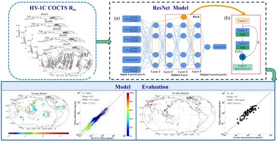
:A residual network (ResNet) model was proposed for estimating Chl-a concentrations in global oceans from the remote sensing reflectance (Rrs) observed by the Chinese ocean color and temperature scanner (COCTS) onboard the HY-1C satellite. A total of 52 images from September 2018 to September 2019 were collected, and the label data were from the multi-task Ocean Color-Climate Change Initiative (OC-CCI) daily products. The results of feature selection and sensitivity experiments show that the logarithmic values of Rrs565 and Rrs520/Rrs443, Rrs565/Rrs490, Rrs520/Rrs490, Rrs490/Rrs443, and Rrs670/Rrs565 are the optimal input parameters for the model. Compared with the classical empirical OC4 algorithm and other machine learning models, including the artificial neural network (ANN), deep neural network (DNN), and random forest (RF), the ResNet retrievals are in better agreement with the OC-CCI Chl-a products. The root-mean-square error (RMSE), unbiased percentage difference (UPD), and correlation coefficient (logarithmic, R(log)) are 0.13 mg/m3, 17.31%, and 0.97, respectively. The performance of the ResNet model was also evaluated against in situ measurements from the Aerosol Robotic Network-Ocean Color (AERONET-OC) and field survey observations in the East and South China Seas. Compared with DNN, ANN, RF, and OC4 models, the UPD is reduced by 5.9%, 0.7%, 6.8%, and 6.3%, respectively.
1. Introduction
Chlorophyll-a (Chl-a) is the main pigment in marine phytoplankton cells and a major indicator of phytoplankton abundance. In areas with high Chl-a concentrations, there are generally relatively large amounts of marine phytoplankton, and marine fishery resources are also relatively abundant. Studies have shown that about 40% of the carbon dioxide (CO2) produced by mineral combustion is absorbed by the ocean, stored in seawater, or converted into organic matter by phytoplankton. The ocean accounts for 71% of the total area of the earth, and the release of only 2% of the CO2 stored in the ocean can double the CO2 content in the atmosphere [1]. As an important participant in the carbon cycle, marine phytoplankton perform photosynthesis to absorb CO2 and generate oxygen for our respiration. Therefore, the ocean plays an important role in reducing atmospheric CO2 and mitigating global warming. At the same time, the number of marine phytoplankton is an important indicator to measure the eutrophication of the water body. When the eutrophication level of the water body is high, the phytoplankton will increase rapidly, causing algae blooms and other disasters. A large number of phytoplankton will block sunlight and affect the growth of other plants, thus affecting the marine ecosystem. Therefore, real-time monitoring of sea surface Chl-a concentration is of great significance for global climate change research and ecological conservation.
The traditional method of obtaining Chl-a concentrations at the sea surface is to use instruments deployed on ships or buoys. Accurate measurement can be achieved in this way, but it is difficult to obtain long-term, continuous, and global information on Chl-a. The progress in ocean color remote sensing technology has provided great convenience and support for monitoring Chl-a concentrations in the ocean [2,3]. By using remote sensing reflectance (Rrs) information from different satellite sensors, researchers have proposed various Chl-a concentration retrieval algorithms. The most widely used algorithm is the empirical model, which usually has high accuracy and is easy to establish. However, due to differences in the distribution of global ocean color elements, empirical models are often only applicable to regions with similar ocean color properties and lack universal applicability [4,5].
In recent years, with the rapid development of artificial intelligence, machine learning methods have been used to estimate Chl-a concentration [6,7,8]. For example, Yu et al. used a neural network to retrieve global sea surface Chl-a concentrations from MODIS (Moderate Resolution Imaging Spectroradiometer) observed Rrs data and compared the results with the OC-CCI (Ocean Color-Climate Change Initiative) product. The root-mean-square error (RMSE) is 0.13 mg/m3 and the coefficient of determination is 0.90 [9]. Also based on MODIS Rrs data, Ye et al. used a two-stage convolutional neural network to calculate Chl-a concentrations in the Pearl River Estuary. Compared with in situ data, the RMSE and coefficient of determination are 0.15 mg/m3 and 0.85, respectively [10]. However, there are still relatively few studies using machine learning, especially deep learning methods, to retrieve sea surface Chl-a concentrations based on Chinese satellite data such as the HY-1 series satellite.
China launched the HY-1C and HY-1D satellites in 2018 and 2020, respectively. By utilizing the Chinese ocean color and temperature scanner (COCTS) onboard these satellites, we are able to observe the ocean color in the same region at least twice a day. Ye et al. merged the empirical OC4 algorithm with the color index (CI) to estimate Chl-a concentrations from COCTS/HY-1C observed Rrs data. Compared with in situ measurements in the East and South China Seas, the correlation coefficient is 0.91, and the unbiased percentage difference (UPD) is 39% [11]. The results indicate that the COCTS has the ability to observe Chl-a concentrations at the sea surface. As far as we know, deep learning models have not been applied to retrieve Chl-a concentrations from COCTS observations before. Can we obtain Chl-a information with higher accuracy from the Rrs data through deep learning methods?
To answer these questions, this study proposed a residual neural network (ResNet) model for global sea surface Chl-a concentration retrieval from COCTS/HY-1C Rrs data by using the OC-CCI product as label data. The performance of the Rrs-based ResNet model was evaluated by comparing the estimation results with independent OC-CCI data and in situ measurements as well.
The rest of the paper is organized as follows. The COCTS/HY-1C observations, OC-CCI product, and in situ measurements of sea surface Chl-a concentrations are described in Section 2. In addition, Section 2 also presents the configuration of the ResNet Chl-a concentration retrieval model, the feature selection method, and the design of comparative experiments in detail. The performance of the model in estimating global sea surface Chl-a concentration is described in Section 3. Section 4 discusses the consistency analysis with the MODIS product and the possible reason for the slight decrease in accuracy. The conclusions and future work are given in Section 5.
2. Materials and Methods
2.1. Data
2.1.1. HY-1C Satellite Data
The HY-1C satellite operates on a sun-synchronous orbit at an altitude of 782 km. The COCTS onboard the satellite has eight visible and near-infrared bands and two thermal infrared bands, with central wavelengths of 412 nm, 443 nm, 490 nm, 520 nm, 565 nm, 670 nm, 750 nm, 865 nm, 10.8 μm, and 12 μm, respectively. The spatial resolution is 1.1 km, and the swath is greater than 2900 km [12]. The L2A data for remote sensing reflectance (Rrs) were calculated through atmospheric correction of the top-of-atmosphere radiance. Totally, 52 COCTS images from September 2018 to September 2019 were collected (https://osdds.nsoas.org.cn/OceanColor, accessed on 6 December 2021). Figure 1 shows an example of Rrs at different visible bands in the Bohai Sea and Yellow Sea.
2.1.2. OC-CCI Dataset
The data utilized for training and validating the ResNet-based Chl-a concentration retrieval model are from the OC-CCI dataset (version 5.0) with a spatial resolution of 4 km (http://www.esa-oceancolour-cci.org/, accessed on 18 February 2022). The process for producing daily sea surface Chl-a concentration products involves the atmospheric correction of multi-band data from MODIS, VIIRS (Visible and Infrared Imager/Radiometer Suite), SeaWiFS (Sea-viewing Wide Field of View Sensor), MERIS (Medium Resolution Imaging Spectrometer), and OLCI (Ocean and Land Colour Instrument) onboard different satellites, followed by the conversion of these data into the bands of MERIS with central wavelengths of 412, 443, 490, 510, 560, and 665 nm. The Rrs data of the five sensors, which were subjected to striping, offset, and correction, were then fused [13]. Finally, the Chl-a concentration was calculated based on the fused Rrs data by using an algorithm that combines the exponential algorithm and the band ratio algorithm [14,15,16]. The OC-CCI Chl-a concentration products have been verified and applied in various regions of the global ocean, indicating that it is a high-quality dataset [17,18,19].
2.1.3. In situ Measurement
In order to further evaluate the performance of the ResNet model, we also collected in situ Chl-a concentration measurements from a field survey in the East and South China Seas from 13 September to 12 October 2018, as well as the AERONET-OC (Aerosol Robotic Network—Ocean Color) data from September 2018 to December 2019 (https://aeronet.gsfc.nas-a.gov/cgi-bin/draw_map_display_seaprism_v3, accessed on 16 June 2022). In the AERONET-OC dataset, Chl-a concentration was calculated using the OC2v4 or regional algorithms based on in situ measured spectral data after strict quality control [20,21,22]. The process and criteria for matching these in situ observations with satellite data are as follows: First, the latitude and longitude of in situ measurements were used to locate the corresponding pixel in the satellite image. Then the average value of satellite-derived Chl-a concentrations centered at this pixel with a 5 × 5 window size was calculated. To ensure the quality of satellite Rrs data, it is required that the effective pixels (i.e., cloud-free, non-land, non-ice, non-solar flare, valid atmospheric correction) in this window exceed 50% and the variation in the internal difference of the data be less than 25% [23]. The time interval between the two datasets is set to less than 2 h. A total of 89 matching data points were obtained, and their spatial distribution is shown in Figure 2.
2.1.4. Data Preprocessing
The construction of a deep learning-based Chl-a concentration retrieval model requires a dataset with a large number of training and testing samples. In this study, to expand the number of data samples, we constructed the match-up data through the following procedures. Firstly, we selected the effective pixel of Rrs data [23]. At the center position of each effective pixel, we then performed the spline interpolation on the OC-CCI product to obtain the corresponding Chl-a concentration data matching the COCTS observed Rrs, and the time window between the two datasets was within 1 day. In this way, the match-up data pairs were ultimately established for model training and validation. Moreover, 32 COCTS images with a total of 762,175 match-up data pairs were randomly selected for training the ResNet model, and the testing dataset consists of 76,620 match-up data pairs from the remaining 22 images. The spatial distribution of the training and testing data is shown in Figure 3.
Due to the fact that the value of Chl-a concentration spans three orders of magnitude, all data were subjected to logarithmic transformation. In order to reduce differences between samples and place them into a distribution with a mean of 0 and a standard deviation of 1, the input data were subjected to Z-score normalization, which involves subtracting the average value of each feature and dividing it by its standard deviation.
2.2. Methodology
In this section, we first present the structure of the ResNet used to estimate sea surface Chl-a concentration from multi-band COCTS data. The permutation feature importance method (PFI) and Bayesian optimization method were adopted to determine the optimal model input parameters and hyperparameters, respectively. Then, comparative experiments were designed to investigate whether the classification of global ocean Chl-a data has an impact on the accuracy of the ResNet model by establishing two sets of deep learning models. The final part of this section introduces the method for evaluating the model’s performance.
2.2.1. Structure of the ResNet and Other Models Settings
There is a complex nonlinear relationship between sea surface Chl-a concentration and satellite-observed signals. A neural network with a multi-layer structure has the advantage of solving such nonlinear problems by continuously adjusting the weight relationship between neurons. Generally, a deep neural network (DNN) can improve the learning ability of a model by increasing the width and depth of the network. But due to the degradation issue of the network, as the depth increases, the training effect may decrease instead. To address this problem, He et al. proposed the ResNet deep learning model [24], which was adopted in this study for estimating global sea surface Chl-a concentrations.
As shown in Figure 4, the ResNet model mainly consists of an input layer, one or more hidden layers, and an output layer. Different from the standard DNN, here we added residual blocks. During the propagation process, the input layer data is used to calculate the output of each layer along the network. Following the second layer, residual blocks are added, and the output result of the second layer is combined with the output result of the fourth layer and input into the fifth layer, achieving skip connections between the data. The gradient is multiplied cumulatively during the backpropagation process to adjust the model. The ResNet has a residual gradient in addition to the target function gradient, which allows the error to be directly fed back to the upper layer. Therefore, even if the model depth increases, the network still maintains good learning ability.
To fully demonstrate the performance of the ResNet model, we also compared this model to the empirical OC4 algorithm and several other machine-learning models, including the artificial neural network (ANN) and random forest (RF) models. ANNs generally have a shallower network structure with fewer layers. The network only has a forward propagation mechanism without reverse feedback; that is, the input layer accepts external parameters, and the hidden layer transmits the results to the output layer after processing, so it is also called a feedforward neural network. The number of hidden layers of the ANN model used in this study is 1, the number of neurons in the hidden layer is 32, the activation function is Tanh, and the initial learning rate is 0.001. Compared with the ANN, the DNN has a reverse parameter adjustment mechanism that can reversely adjust the weights of each layer of the model based on the output. The network has a relatively larger number of hidden layers (set at 3, and the number of neurons in the hidden layer is 32). The activation function and the initial learning rate are the same as the ANN. The RF model combines multiple weak algorithms with Bagging [25]. The number of estimator trees was set at 50. The minimum number of samples for split nodes is 2, the minimum number of samples at leaf nodes is 1, and the method for selecting the maximum feature number is sqrt.
2.2.2. Feature Selection and Hyperparameter Determination Methods
There is a significant difference in the spectral characteristics of Chl-a between 400 and 700 nm. In general, the absorption peak appears near 440 nm and 670 nm, and the strong reflection peak is near 550 nm. Based on the spectral characteristics of Chl-a, different algorithms have been proposed to estimate sea surface Chl-a concentrations using Rrs data or their ratios in different bands. Which band or band ratio contributes more to the ResNet-based Chl-a concentration retrieval model? In this study, we used permutation feature importance to assess the importance of each band of data [26,27]. PFI is a method to determine the importance of a feature in a trained model by randomly shuffling the values of one feature while keeping the order of other features unchanged. The importance of a feature was determined by the degree of decrease in model performance that results from changing the feature sequence. If the model’s performance decreases significantly after changing a feature, it indicates that the feature is more important to the model. Based on the band configuration of COCTS, we mainly analyzed the importance of Rrs443, Rrs490, Rrs520, Rrs565, Rrs670 and the ratios between the (Rrs490/Rrs443, Rrs520/Rrs443, Rrs520/Rrs490, Rrs565/Rrs443, Rrs565/Rrs490, Rrs565/Rrs520, Rrs670/Rrs443, Rrs670/Rrs490, Rrs670/Rrs520, and Rrs670/Rrs565).
The performance of a deep learning model not only depends on the input parameters but is also closely related to the selection of model hyperparameters. In order to develop a ResNet model with excellent performance, the hyperparameters such as model width, the number of residual blocks, and learning rate were determined by the Bayesian optimization method, and the type of residual block was determined by the control variable method. After testing, we set the model width to 32 and the initial learning rate to 0.001, with a 2-layer skip-connection residual block as shown in Figure 4b.
2.2.3. Design of Comparative Experiments
Some studies have shown that establishing separate models based on the classification results of Rrs may improve the model’s performance. The existing classification methods generally classify water bodies based on spectral information and then construct retrieval models [28,29,30]. The spectral characteristics of nearshore and open ocean waters are different; to compare the performance of unclassified and classified ResNet models, we processed the training and testing datasets in two ways: (1) Treating all Rrs data as a whole, and (2) dividing the data into two types, namely nearshore water and ocean (200 km offshore). Accordingly, non-classification models (ResNet1) and classification-based models (ResNet2) were designed.
2.2.4. Model Performance Evaluation Method
The performance of the ResNet model is evaluated using the root-mean-square error (RMSE), unbiased percentage difference (UPD), and correlation coefficient (logarithmic, R(log)). They are expressed as:
where and are model estimated Chl-a concentration and the true value, respectively; and represent the mean values of change in the model-derived Chl-a concentration and the true value, respectively; represents the total number of the testing data.
3. Results
3.1. What Are the Optimal Model Input Parameters?
Figure 5 shows the importance of each input parameter to the non-classification ResNet model based on the PFI analysis. The first eight parameters with higher importance are , , , , , , , . In order to determine the optimal input parameters, five comparative experiments were conducted by selecting the first four to eight parameter combinations as model inputs, respectively. The results of the testing dataset are shown in Table 1. The ResNet model with the first six parameters as inputs has the highest accuracy. These parameters were considered the optimal model inputs and used in the following experiments.
3.2. Performance of the ResNet Model
In this section, the performance of the ResNet model was evaluated based on different datasets, including OC-CCI products and in situ measurements. The model was also compared with other machine learning models, including ANN, DNN, RF, and the classical empirical OC4 algorithm, which was widely used and developed based on SeaWiFS data [15,20,31].
3.2.1. Performance Evaluation with OC-CCI Products
Figure 6 shows the accuracy of ResNet and DNN models in estimating global sea surface Chl-a concentrations against OC-CCI products. In general, except for classification-based DNN models, almost all types of models perform well with RMSE smaller than 0.25 mg/m3, UPD less than 25%, and R(log) higher than 0.94. The overall performance of non-classification models is superior to that of classification models. Therefore, in the following discussion, we will focus on analyzing the non-classification model established by taking all the training data as a whole.
Figure 7 shows the scatter density plot between sea surface Chl-a concentrations retrieved using different models and the OC-CCI product in the testing dataset. The RMSEs (0.13–0.14 mg/m3) of Chl-a concentrations retrieved by neural networks are similar and slightly smaller than those retrieved by RF and OC4 models. Although the correlation coefficients of all model estimations are above 0.90, the ResNet-derived UPD (17.31%) is the smallest. When the Chl-a concentration is less than 0.1 mg/m3, the ANN underestimates the Chl-a concentration, while the OC4 overestimates the concentration.
Figure 8 shows the comparison between the frequency distribution of Chl-a estimation results and that of the OC-CCI product. Compared with the other models, the frequency distribution of ResNet-retrieved results is much closer to that of OC-CCI. The DNN, ANN, and RF models capture the distribution well when the Chl-a concentration is greater than 0.1 mg/m3. When the Chl-a concentration is greater than 0.2 mg/m3, all models can accurately reproduce its frequency distribution. Although the accuracy of the ResNet and DNN models shown in Figure 7 is similar, combined with Figure 8, it can be found that the ResNet estimation results are in better agreement with the OC-CCI product, indicating that this model has higher performance than the other machine-learning or empirical models.
3.2.2. Performance Evaluation with In Situ Measurements
The scatter plot between Chl-a concentrations derived from different models and in situ measurements is shown in Figure 9. Comparing Figure 7 with Figure 9, one can see that the error against field data is a little higher. This may be because the in situ data are mostly located in offshore areas (Figure 2). However, the correlation coefficient between the ResNet estimations and observations still reaches 0.90, and the RMSE is the smallest among all models. The UPD is 36.14%, which is 5.9%, 0.7%, 6.8%, and 6.3% lower than that obtained by the DNN, ANN, RF, and OC4 models, respectively.
4. Discussion
4.1. Consistency Evaluation with MODIS Observation
A case study was carried out in the Bohai Sea and Yellow Sea to further demonstrate the consistency between COCTS-derived Chl-a concentrations using the ResNet model and the MODIS product of Chl-a concentrations obtained from the OC3M algorithm [32]. We selected satellite data on 24 January 2019, as an example. The COCTS/HY-1C image was acquired at 02:45 UTC, and the MODIS/Aqua image was acquired about 5 minutes later. As shown in Figure 10a,b, the spatial pattern of the Chl-a concentration observed by COCTS is generally consistent with MODIS observations. High concentrations distributed along the coastal areas can be observed from both sensors. Quantitative analysis shows that the two datasets are in good agreement, with a UPD of less than 17% and a correlation coefficient of 0.88 (Figure 10c).
4.2. Reasons for Different Accuracy when Using Different Data Validation
Comparing Figure 7 and Figure 9, one can see that the error of the ResNet-derived Chl-a concentration against in situ measurements is a little higher. This may be because the field observations are mostly located in nearshore areas (Figure 2), where the ocean color attributes are more complex and quite different from those in the open ocean [10,33,34], To further investigate the performance of the ResNet model in nearshore waters, we analyzed the variation of UPD with offshore distance. As shown in Figure 11, the locations of in situ measurements in Figure 9 can be divided into three parts according to their distance from the coastline: <50 km (81 points), 50–100 km (5 points), and 100–200 km (3 points). It is obvious that as the offshore distance increases, the UPD shows a significantly downward trend. Due to the fact that most training and testing data used to construct the ResNet model are distributed in the open ocean, the model does not work as well in nearshore waters as it does in the open ocean, but it is still within a reasonable error range. With the collection of more field observations in the near future, it is expected to improve the accuracy of the ResNet model in nearshore waters.
5. Conclusions
In this study, a ResNet method for retrieving global sea surface Chl-a concentrations based on Rrs by COCTS onboard the HY-1C satellite was developed. The PFI method was used to determine the contribution of different band data to the model’s performance. Additional sensitivity analysis shows that the optimal model input parameters for the Rrs-based model are Rrs520/Rrs443, Rrs565/Rrs490, Rrs520/Rrs490, Rrs490/Rrs443, Rrs565, Rrs670/Rrs565. The results of comparative experiments indicate that higher accuracy can be obtained by taking the training data as a whole instead of dividing it into two types: offshore and open ocean waters.
Compared with the OC-CCI Chl-a product, the RMSE and UPD of the Chl-a concentration estimated from Rrs using the optimal ResNet model are 0.13 mg/m3 and 17.31%, respectively, a little smaller than those of the DNN model without the residual blocks. The correlation coefficient R(log) is up to 0.97. The Rrs-based ResNet model was also evaluated using in situ measurements as independent data. Compared with DNN, ANN, RF, and OC4 models, the UPD is reduced by 5.9%, 0.7%, 6.8%, and 6.3%, respectively, further indicating the good performance of our model.
In the near future, in order to further improve the performance of the ResNet model in coastal waters, more in situ measurement data of sea surface Chl-a concentration will be collected to expand the number of training and testing samples. Moreover, HY-1C is also equipped with a CZI sensor. The CZI bands with center wavelengths of 450 nm and 560 nm, respectively, can also be used to retrieve the concentration of Chl-a on the sea surface with higher resolution than COCTS sensors. In future studies, we will consider building a Chl-a concentration retrieval model at the sea surface based on the HY1C CZI.
Author Contributions
Conceptualization, Q.X. and X.Y. (Xiaomin Ye); methodology, G.Y., X.Y. (Xiaomin Ye) and Q.X.; software, G.Y. and S.X.; investigation, X.Y. (Xiaobin Yin), and S.X.; writing—original draft preparation, G.Y.; writing—review and editing, X.Y. (Xiaomin Ye), X.Y. (Xiaobin Yin), Q.X. and S.X.; supervision, Q.X. and X.Y. (Xiaobin Yin). All authors have read and agreed to the published version of the manuscript.
Funding
This research was funded by Sanya Yazhou Bay Science and Technology City through Grant SKJC-2022-01-001 and the National Natural Science Foundation of China through Grants T2261149752 and 41976163.
Data Availability Statement
Not applicable.
Acknowledgments
The authors would like to thank the National Satellite Ocean Application Center for providing HY-1C/COCTS Level-1,2 data, the European Space Agency for providing Ocean Color-Climate Change Initiative (OC-CCI) Chlorophyll-a concentration data, the NASA Goddard Space Center for providing MODIS data, and the Goddard Space Flight Center for providing AERONET-OC Chlorophyll-a concentration data.
Conflicts of Interest
The authors declare no conflict of interest.
References
- Yang, Y.; Li, Y.; Pan, J. Characteristics of an Open Complex Giant System-Carbon Cycling System in the Ocean. Complex Syst. Complex. Sci. 2004, 1, 10. [Google Scholar]
- Silveira Kupssinsku, L.; Thomassim Guimaraes, T.; Menezes de Souza, E.; Zanotta, D.C.; Roberto Veronez, M.; Gonzaga, L., Jr.; Mauad, F.F. A Method for Chlorophyll-a and Suspended Solids Prediction through Remote Sensing and Machine Learning. Sensors 2020, 20, 2125. [Google Scholar] [CrossRef] [Green Version]
- El-Alem, A.; Chokmani, K.; Laurion, I.; El-Adlouni, S.E. Comparative Analysis of Four Models to Estimate Chlorophyll-a Concentration in Case-2 Waters Using MODerate Resolution Imaging Spectroradiometer (MODIS) Imagery. Remote Sens. 2012, 4, 2373–2400. [Google Scholar] [CrossRef] [Green Version]
- Clay, S.; Pena, A.; DeTracey, B.; Devred, E. Evaluation of Satellite-Based Algorithms to Retrieve Chlorophyll-a Concentration in the Canadian Atlantic and Pacific Oceans. Remote Sens. 2019, 11, 2609. [Google Scholar] [CrossRef] [Green Version]
- Sauer, M.; Roesler, C.; Werdell, J.; Barnard, A. Under the hood of satellite empirical chlorophyll a algorithms: Revealing the dependencies of maximum band ratio algorithms on inherent optical properties. Opt. Express. 2012, 20, 20920–20933. [Google Scholar] [CrossRef] [PubMed]
- Zhang, T. Evaluating the performance of artificial neural network techniques for pigment retrieval from ocean color in Case I waters. J. Geophys. Res. Oceans 2003, 108, 3286. [Google Scholar] [CrossRef]
- Syariz, M.A.; Lin, C.-H.; Nguyen, M.V.; Jaelani, L.M.; Blanco, A.C. WaterNet: A Convolutional Neural Network for Chlorophyll-a Concentration Retrieval. Remote Sens. 2020, 12, 1966. [Google Scholar] [CrossRef]
- Ali, K.A.; Moses, W.J. Application of a PLS-Augmented ANN Model for Retrieving Chlorophyll-a from Hyperspectral Data in Case 2 Waters of the Western Basin of Lake Erie. Remote Sens. 2022, 14, 3729. [Google Scholar] [CrossRef]
- Yu, B.; Xu, L.; Peng, J.; Hu, Z.; Wong, A. Global chlorophyll-a concentration estimation from moderate resolution imaging spectroradiometer using convolutional neural networks. J. Appl. Remote Sens. 2020, 14, 034520. [Google Scholar] [CrossRef]
- Ye, H.; Tang, S.; Yang, C. Deep Learning for Chlorophyll-a Concentration Retrieval: A Case Study for the Pearl River Estuary. Remote Sens. 2021, 13, 3717. [Google Scholar] [CrossRef]
- Ye, X.; Liu, J.; Lin, M.; Ding, J.; Zou, B.; Song, Q. Global Ocean Chlorophyll-a Concentrations Derived From COCTS Onboard the HY-1C Satellite and Their Preliminary Evaluation. IEEE Trans. Geosci. Electron. 2021, 59, 9914–9926. [Google Scholar] [CrossRef]
- Song, Q.; Chen, S.; Xue, C.; Lin, M.; Du, K.; Li, S.; Ma, C.; Tang, J.; Liu, J.; Zhang, T.; et al. Vicarious calibration of COCTS-HY1C at visible and near-infrared bands for ocean color application. Opt. Express. 2019, 27, A1615–A1626. [Google Scholar] [CrossRef] [PubMed]
- Sathyendranath, S.; Jackson, T.; Brockmann, C.; Brotas, V.; Calton, B.; Chuprin, A.; Clements, O.; Cipollini, P.; Danne, O.; Dingle, J.; et al. ESA Ocean Colour Climate Change Initiative (Ocean_Colour_CCI): Version 5.0 Data. NERC EDS Centre for Environmental Data Analysis, 2021. Available online: http://climate.esa.int/en/projects/ocean-colour/key-documents/ (accessed on 15 March 2023).
- Gordon, H.; Morel, A. Remote assessment of ocean color for interpretation of satellite visible imagery: A review. Phys. Earth Planet. Int. 1983, 37, 292. [Google Scholar]
- O’Reilly, J.; Maritorena, S.; Mitchell, B.G.; Siegel, D.; Carder, K.; Garver, S.A.; Kahru, M.; Mcclain, C. Ocean color chlorophyll algorithms for SeaWiFS. J. Geophys. Res. C. 1998, 103, 937–953. [Google Scholar] [CrossRef] [Green Version]
- Hu, C.; Lee, Z.; Franz, B. Chlorophyll a algorithms for oligotrophic oceans: A novel approach based on three-band reflectance difference. J. Geophys. Res. C Oceans 2012, 117, C01011. [Google Scholar] [CrossRef] [Green Version]
- Ferreira, A.; Brotas, V.; Palma, C.; Borges, C.; Brito, A.C. Assessing Phytoplankton Bloom Phenology in Upwelling-Influenced Regions Using Ocean Color Remote Sensing. Remote Sens. 2021, 13, 675. [Google Scholar] [CrossRef]
- Keerthi, M.G.; Prend, C.J.; Aumont, O.; Lévy, M. Annual variations in phytoplankton biomass driven by small-scale physical processes. Nat. Geosci. 2022, 15, 1027–1033. [Google Scholar] [CrossRef]
- Pitarch, J.; Bellacicco, M.; Marullo, S.; Van Der Woerd, H.J. Global maps of Forel-Ule index, hue angle and Secchi disk depth derived from twenty-one years of monthly ESA-OC-CCI data. Earth Syst. Sci. Data 2021, 13, 481–490. [Google Scholar] [CrossRef]
- O’Reilly, J. Ocean color chlorophyll a algorithms for SeaWiFS, OC2, and OC4: Version 4. SeaWiFS Postlaunch Calibration Valid. Anal. 2000, 11, 9–23. [Google Scholar]
- Zibordi, G.; Berthon, J.-F.; Mélin, F.; D’Alimonte, D.; Kaitala, S. Validation of satellite ocean color primary products at optically complex coastal sites: Northern Adriatic Sea, Northern Baltic Proper and Gulf of Finland. Remote Sens. Environ. 2009, 113, 2574–2591. [Google Scholar] [CrossRef]
- Zibordi, G.; Mélin, F.; Berthon, J.-F.; Talone, M. In situ autonomous optical radiometry measurements for satellite ocean color validation in the Western Black Sea. Ocean Sci. 2015, 11, 275–286. [Google Scholar] [CrossRef] [Green Version]
- Bailey, S.W.; Werdell, P.J. A multi-sensor approach for the on-orbit validation of ocean color satellite data products. Remote Sens. Environ. 2006, 102, 12–23. [Google Scholar] [CrossRef]
- He, K.; Zhang, X.; Ren, S.; Sun, J. Deep residual learning for image recognition. In Proceedings of the IEEE Conference on Computer Vision and Pattern Recognition, Las Vegas, NV, USA, 10 December 2015. [Google Scholar]
- Brownlee, J. Bagging and Random Forest Ensemble Algorithms for Machine Learning. 2016, pp. 4–22. Available online: https://machinelearningmastery.com/bagging-and-random-forest-ensemble-algorithms-for-machine-learning/ (accessed on 26 June 2023).
- Yang, J.-B.; Shen, K.-Q.; Ong, C.-J.; Li, X.-P. Feature Selection for MLP Neural Network: The Use of Random Permutation of Probabilistic Outputs. IEEE Trans. Neural Netw. 2009, 20, 1911–1922. [Google Scholar] [CrossRef]
- Fisher, A.; Rudin, C.; Dominici, F. All Models are Wrong, but Many are Useful: Learning a Variable’s Importance by Studying an Entire Class of Prediction Models Simultaneously. J. Mach. Learn. Res. JMLR 2019, 20, 1–81. [Google Scholar]
- Le, C.; Li, Y.; Zha, Y.; Sun, D.; Huang, C.; Zhang, H. Remote estimation of chlorophyll a in optically complex waters based on optical classification. Remote Sens. Environ. 2011, 115, 725–737. [Google Scholar] [CrossRef]
- Neil, C.; Spyrakos, E.; Hunter, P.D.; Tyler, A.N. A global approach for chlorophyll-a retrieval across optically complex inland waters based on optical water types. Remote Sens. Environ. 2019, 229, 159–178. [Google Scholar] [CrossRef]
- Zhang, F.; Li, J.; Shen, Q.; Zhang, B.; Tian, L.; Ye, H.; Wang, S.; Lu, Z. A soft-classification-based chlorophyll-a estimation method using MERIS data in the highly turbid and eutrophic Taihu Lake. Int. J. Appl. Earth Obs. Geoinf. 2019, 74, 138–149. [Google Scholar] [CrossRef]
- O’Reilly, J.E.; Werdell, P.J. Chlorophyll Algorithms for Ocean Color Sensors—Oc4, Oc5 & Oc6. Remote Sens. Environ. 2019, 229, 32–47. [Google Scholar] [CrossRef]
- Hooker, S.; Firestone, E.; Mcclain, C.; Kwiatkowska, E.; Barnes, R.; Eplee, R.; Elaine, R.; Patt, F.; Robinson, W.; Wang, M.; et al. SeaWiFS Postlaunch Calibration and Validation Analyses Part 1. 2000; pp. 4–12. Available online: https://www.researchgate.net/publication/24293669_SeaWiFS_Postlaunch_Calibration_and_Validation_Analyses (accessed on 25 August 2022).
- Odermatt, D.; Gitelson, A.; Brando, V.E.; Schaepman, M. Review of constituent retrieval in optically deep and complex waters from satellite imagery. Remote Sens. Environ. 2012, 118, 116–126. [Google Scholar] [CrossRef] [Green Version]
- Su, H.; Lu, X.; Chen, Z.; Zhang, H.; Lu, W.; Wu, W. Estimating Coastal Chlorophyll-A Concentration from Time-Series OLCI Data Based on Machine Learning. Remote Sens. 2021, 13, 576. [Google Scholar] [CrossRef]
Figure 1.
HY-1C/COCTS observation in the Bohai Sea and Yellow Sea at 02:53 UTC on November 11, 2019. (a–e): Rrs at central wavelengths of 443, 490, 520, 565, and 670 nm, respectively.
Figure 1.
HY-1C/COCTS observation in the Bohai Sea and Yellow Sea at 02:53 UTC on November 11, 2019. (a–e): Rrs at central wavelengths of 443, 490, 520, 565, and 670 nm, respectively.

Figure 2.
Spatial distribution of in situ measurements of sea surface Chl-a concentration matched with COCTS/HY-1C observations. Red and blue dots denote the locations of AERONET-OC data and field surveys in the East and South China Seas, respectively.
Figure 2.
Spatial distribution of in situ measurements of sea surface Chl-a concentration matched with COCTS/HY-1C observations. Red and blue dots denote the locations of AERONET-OC data and field surveys in the East and South China Seas, respectively.

Figure 3.
Spatial distribution of OC-CCI products matched with COCTS/HY-1C data: (a) training dataset; (b) testing dataset.
Figure 3.
Spatial distribution of OC-CCI products matched with COCTS/HY-1C data: (a) training dataset; (b) testing dataset.

Figure 4.
(a) Schematic diagram of ResNet for sea surface Chl-a concentration estimation. The yellow circle represents the output of the second layer. (b) Schematic diagram of the residual block.
Figure 4.
(a) Schematic diagram of ResNet for sea surface Chl-a concentration estimation. The yellow circle represents the output of the second layer. (b) Schematic diagram of the residual block.

Figure 5.
Importance of different model input parameters based on the PFI analysis.

Figure 6.
(a) RMSE, (b) UPD, and (c) R(log) between sea surface Chl-a concentration estimated using the ResNet or DNN model and OC-CCI products. The numbers 1 and 2 after the model’s name represent the non-classification model and classification model, respectively.
Figure 6.
(a) RMSE, (b) UPD, and (c) R(log) between sea surface Chl-a concentration estimated using the ResNet or DNN model and OC-CCI products. The numbers 1 and 2 after the model’s name represent the non-classification model and classification model, respectively.

Figure 7.
Comparison of sea surface Chl-a concentration retrieved using (a) ResNet, (b) DNN, (c) ANN, (d) RF and (e) OC4 and the OC-CCI product.
Figure 7.
Comparison of sea surface Chl-a concentration retrieved using (a) ResNet, (b) DNN, (c) ANN, (d) RF and (e) OC4 and the OC-CCI product.

Figure 8.
Frequency distribution of sea surface Chl-a concentration retrieved using (a) ResNet, (b) DNN, (c) ANN, (d) RF and (e) OC4 and that of the OC-CCI product.
Figure 8.
Frequency distribution of sea surface Chl-a concentration retrieved using (a) ResNet, (b) DNN, (c) ANN, (d) RF and (e) OC4 and that of the OC-CCI product.

Figure 9.
Comparison of sea surface Chl-a concentrations retrieved using (a) ResNet, (b) DNN, (c) ANN, (d) RF and (e) OC4 and in situ measurements. Black and blue dots denote measurements from the AERONET-OC data and field survey in the East and South China Seas, respectively.
Figure 9.
Comparison of sea surface Chl-a concentrations retrieved using (a) ResNet, (b) DNN, (c) ANN, (d) RF and (e) OC4 and in situ measurements. Black and blue dots denote measurements from the AERONET-OC data and field survey in the East and South China Seas, respectively.

Figure 10.
(a) Sea surface Chl-a concentration in the Bohai Sea and Yellow Sea estimated from COCTS/HY-1C at 02:45 UTC on 24 January 2019. (b) Terra/MODIS product at 02:50 UTC on the same day (http://oceancolor.gsfc.nasa.gov/, accessed on 12 December 2022). (c) Scatter plot between COCTS and MODIS-derived Chl-a concentrations.

Figure 11.
Variation of the UPD of the ResNet-derived Chl-a concentration against in situ measurements with offshore distance.
Figure 11.
Variation of the UPD of the ResNet-derived Chl-a concentration against in situ measurements with offshore distance.


Table 1.
The accuracy of ResNet1 models with different input parameters. In models ResNet1_4 to ResNet1_8, the first four to eight parameters shown in Figure 5 were used as model inputs.
Table 1.
The accuracy of ResNet1 models with different input parameters. In models ResNet1_4 to ResNet1_8, the first four to eight parameters shown in Figure 5 were used as model inputs.
| Model ID | ResNet1_4 | ResNet1_5 | ResNet1_6 | ResNet1_7 | ResNet1_8 |
|---|---|---|---|---|---|
| R(log) | 0.95 | 0.95 | 0.97 | 0.95 | 0.95 |
| RMSE (mg/m3) | 0.14 | 0.19 | 0.13 | 0.14 | 0.13 |
| UPD (%) | 21.14 | 19.16 | 17.31 | 19.61 | 20.76 |
Disclaimer/Publisher’s Note: The statements, opinions and data contained in all publications are solely those of the individual author(s) and contributor(s) and not of MDPI and/or the editor(s). MDPI and/or the editor(s) disclaim responsibility for any injury to people or property resulting from any ideas, methods, instructions or products referred to in the content. |
© 2023 by the authors. Licensee MDPI, Basel, Switzerland. This article is an open access article distributed under the terms and conditions of the Creative Commons Attribution (CC BY) license (https://creativecommons.org/licenses/by/4.0/).
Share and Cite
MDPI and ACS Style
Yang, G.; Ye, X.; Xu, Q.; Yin, X.; Xu, S. Sea Surface Chlorophyll-a Concentration Retrieval from HY-1C Satellite Data Based on Residual Network. Remote Sens. 2023, 15, 3696. https://doi.org/10.3390/rs15143696
AMA Style
Yang G, Ye X, Xu Q, Yin X, Xu S. Sea Surface Chlorophyll-a Concentration Retrieval from HY-1C Satellite Data Based on Residual Network. Remote Sensing. 2023; 15(14):3696. https://doi.org/10.3390/rs15143696
Chicago/Turabian StyleYang, Guiying, Xiaomin Ye, Qing Xu, Xiaobin Yin, and Siyang Xu. 2023. "Sea Surface Chlorophyll-a Concentration Retrieval from HY-1C Satellite Data Based on Residual Network" Remote Sensing 15, no. 14: 3696. https://doi.org/10.3390/rs15143696
Note that from the first issue of 2016, this journal uses article numbers instead of page numbers. See further details here.