
Three-Dimensional Modelling of Past and Present Shahjahanabad through Multi-Temporal Remotely Sensed Data


Faculty of Geo-Information Science and Earth Observation (ITC), University of Twente, 7514 Enschede, The Netherlands
*
Author to whom correspondence should be addressed.
Remote Sens. 2023, 15(11), 2924; https://doi.org/10.3390/rs15112924
Submission received: 2 May 2023
/
Revised: 1 June 2023
/
Accepted: 1 June 2023
/
Published: 3 June 2023
(This article belongs to the Special Issue Application of Remote Sensing in Cultural Heritage Research)
Abstract
:Cultural heritage is under tremendous pressure in the rapidly growing and transforming cities of the global south. Historic cities and towns are often faced with the dilemma of having to preserve old monuments while responding to the pressure of adapting itself to a modern lifestyle, which often results in the loss of cultural heritage. Indian cities such as Delhi possess a rich legacy of tangible heritage, traditions, and arts, which are reflected in their present urban form. The creation of temporal 3D models of such cities not only provides a platform with which one can experience the past, but also helps to understand, examine, and improve its present deteriorating state. However, gaining access to historical data to support the development of city-scale 3D models is a challenge. While data gaps can be bridged by combining multiple data sources, this process also presents considerable technical challenges. This paper provides a framework to generate LoD-2 (level-of-detail) 3D models of the present (the 2020s) and the past (the 1970s) of a heritage mosque surrounded by a dense and complex urban settlement in Shahjahanabad (Old Delhi) by combining multiple VHR (very high resolution) satellite images. The images used are those of Pleiades and Worldview-1 and -3 (for the present) and HEXAGON KH-9 declassified spy images (for the past). The chronological steps are used to extract the DSMs and DTMs that provide a base for the 3D models. The models are rendered, and the past and present are visualized using graphics and videos. The results reveal an average increase of 80% in the heights of the built structures around the main monument (mosque), leading to a loss in the visibility of this central mosque.
1. Introduction
1.1. Importance of 3D Modelling in Heritage Conservation
Heritage plays an essential role in understanding the historical importance of a place. It holds social and historical values that people often perceive as part of their identity and pride [1]. The digital documentation of heritage not only helps in understanding the evolution of a place through time but also provides a base for the implementation of conservation tools [2,3]. In 2015, the United Nations included heritage conservation (SDG 11.4) as an essential contributor toward sustainable development (SDG 11) [4]. This recognition identifies the protection of cultural heritage as one of the underlining approaches to achieving inclusive, safe, and sustainable cities [4]. Therefore, it becomes essential to develop tools that facilitate the tasks of conservationists, environmentalists, and experts in similar domains to achieve the SDGs set by the United Nations.
The geographic information system (GIS) has long been used to support the planning and preservation of cities [1,5]. The digitization of historical maps, archived satellite imageries, old photographs, and ancient paintings provides valuable resources for heritage conservation, but these are often limited to 2D visualization [6]. Adding a third dimension can not only help in the better visualization of structures and landscapes, it can also help us understand a site’s history and its evolution [3]. In addition, such 3D reconstructions can also provide a base for the implementation of the tools for heritage conservation [3,7,8]. In addition to visualization purposes, 3D models open the scope of the use of exploratory tools that are otherwise limited in 2D documentation. Some of the applications of 3D models include flood simulation analysis, wind analysis, solar potential analysis, shadow analysis, or visibility analysis [9].
1.2. Visibility: An Important Factor for Heritage Conservation and Cultural Identity
The visibility of space in an urban environment becomes crucial in defining its interaction with the user. The spatial experience of any space is defined by how a user forms their visual impression. Kevin Lynch, in his book The Image of the City, describes the importance of visual perception in creating a mental representation of a city [10]. Historical monuments were also built to maintain their visibility from far-off distances. The grandness of the structure often glorified the personas of the kings and emperors [11]. Studies also show that large monumental buildings evoke a sense of awe that triggers the perception of a freeze in the brain [12]. The main monument, which forms the center of our study area, was built on a plinth 30 feet above ground level [13]. The street avenues were built such that the three magnificent domes of the mosque were visible while heading toward its entrance [13]. With the increase in urbanization and the further addition of taller buildings in its surroundings, the visibility of the mosque has become hindered to a large extent. Globally, many cities place a high value on the importance of the visibility of historic monuments. For example, London has made policies that protect the views; these policies restrict construction and the addition of new taller buildings that obstruct the view of old heritage monuments [14]. These law recognizes the protection of views as part of heritage preservation, and this contributes to the achievement of a sustainable development goal (SDG 11.4) [1]. Moreover, the view of the landmarks of prominent historic structures creates in people a sense of identity and belonging. It also helps to create mental maps in people’s minds that produce long-lasting impressions of that place. The visibility of such landmarks not only increases the aesthetics of the places but also promotes and boosts tourism.
1.3. Past Attempts of Generating Models from Declassified Satellite Images
Conventional stereo-matching (SGM) techniques to produce digital surface models (DSMs) from very high resolution (VHR) satellite images are commonly used to generate 3D city models [15]. Modern satellite stereo images often come with RPCs (rational polynomial coefficients), which provide the embedded information required for DSM generation. These files can then be used to automatically process images to produce high-quality elevation models. However, when working with old satellite systems, these parameters are often unknown; therefore, the process of DSM generation in such cases is not that straightforward.
In the recent past, many attempts have been made to create digital elevation models (DEMs) from the archives of declassified US spy satellite imagery to study surface topological changes [3,4]. The presence of stereo panoramic cameras in missions such as HEXAGON KH-4B or KH-9 produced high-resolution stereo images which were suitable for producing 3D topographical data [5]. However, due to the old camera frames, which were prone to relatively large distortions and missing metadata, it was difficult to extract height information and efficiently utilize their full potential [5]. There have been attempts to create elevation models from archival satellite stereo pairs, but none of these explicitly explained its methodology. Moreover, the resultant generated DEMs were of coarser resolutions as none of them used images of sub-metric resolution. Jesse and Jackson derived 10 m DEMs from CORONA KH-4B images with a ground sample distance (GSD) of 1.83 [5]. In another research work, the structure from motion (SfM) technique was used to produce 5 m DSMs from CORONA KH-4A (2.7 m GSD) images [6].
Therefore, this paper aims to produce very high resolution DSMs of the present (the 2020s) and the past (the 1970s) by combining datasets from multiple sources and time. The paper provides a framework to use the generated DSMs to further refine and obtain DTMs (digital terrain models) using a deep learning method called ResDepth [16]. Finally, the DSMs and DTMs are used to generate two comparative LoD-2 (level of detail) 3D city models of the same. CityGML (City Geographic Markup Language), a standard data structure format for 3D models, defines level of detail as the details used to visualize urban objects. Different scales of LoD define the amount of information added to the model [9]. Figure 1 shows the differences between the types of LoD described under CityGML.
LoD-0 refers to an elevation model (DTM/DSM) with a draped image. LoD-1 is simply extruded blocks representing buildings without texture. LoD-2 adds up more information by providing shaped roof structures with texture. In LoD-3, details are added to the facades to depict the balconies and windows. Lastly, LoD-4 encapsulates BIM (building information modelling), where the modelling goes beyond the outer facades to model the interior structures of the buildings. In this paper, a framework is provided to create LoD-2 models with DSMs, DTMs, building footprints, VHR satellite images and Google Earth, using deep learning to produce models with defined roof shapes and textures.
2. Materials and Methods
2.1. Study Area
The study area lies in the heart of Delhi, India’s capital city. Covering roughly eight square kilometers, Shahjahanabad, which once lay adjacent to the river Yamuna, is now about 1.5 km away from it, due to the eastward shift of the river. With a population of over 250,000 (in 2020), the densely packed structures and narrow streets and lanes and the almost non-existent vegetation cover give Shahjahanabad a slum-like appearance [18]. The entire city comprises numerous irregularly shaped buildings with moderately flat roofs. Due to the challenging nature and complex geometries of the urban morphology, the methodology was tested in a select part of the city. The selection was based on a suitable (very complex) historic residential area in order to perform the visibility analysis on one of the main heritage monuments within the city. The criterion was to select a monument that had remained static through time but had witnessed changes around itself. Therefore, an area of a 300 m radius was delineated around the Principal Mosque—the ‘Jama Masjid’—to test our methodology (Figure 2).
Jama Masjid, a Culturally Rich Heritage
Completed in 1656 CE, Jama Masjid, which is still the biggest mosque in Delhi, was the religious and cultural heart of Shahjahanabad. The structure was built on a 30-foot-high (9.1 m) plinth measuring 80 × 27.5 m [13]. As the religious center of the city, the mosque was built on a hillock (Bhojala Pahadi) that gave it a significance which most pre-modern religious places commanded [13]. The three main marble domes on the mosque symbolized this landmark of Shahjahanabad that was visible from miles away. The mosque was named ‘Masjid-e-Jahanumma’—which literally meant a mosque commanding the world’s view [13]. The monument, which survived under different authoritative powers (namely the Mughals, the British, and those of post-independence India), is important to the city’s heritage. Figure 3 shows the evolution of space around Jama Masjid from the 1880s to the present. Furthermore, Jama Masjid is a visible landmark facilitating internal orientation in a complex and densely built-up area. The streets, which had clear views of its domes and minarets in the time gone by, now offer somewhat hindered views because of the increased heights of the buildings. Thus, the availability of the data, the importance of the monument as a landmark, and the rich heritage of the place make it an appropriate choice for reconstruction.
2.2. Methodology
The generation of the two city models required different approaches and strategies as both differed with respect to the selection of data sources, year, method of processing, and texturing. The first step was to explore the available data sources for building the present and past 3D models. The selection of data was based on the following points:
- Data sources that could potentially produce the same level-of-detail models for both the present and the past.
- Data sources that could follow the same (more or less) methodological framework.
- The use of remote sensing data sources and methodologies, including the use of deep learning.
Based on the above aims, satellite images were used as the base of the two models as these were common sources in the acquisition of both sets of data. This section gives a brief description of the methodologies with schematics describing the generation of the two models.
City Model Generation: 2020s and 1970s
Five satellite images from Pleiades and Worldview were integrated to produce the DSM using the conventional semi-global matching (SGM) approach. After creating the DSM, a digital terrain model (DTM) was extracted by interpolation after applying a deep learning method. Then, a normalized DSM (nDSM) was created from the DSM and DTM containing the absolute heights of the buildings. These values were used as attributes for the building footprints of 2018. The vector file was later converted into a multipatch file (compatible with ArcGIS Pro) to obtain a plain 3D model without texture. Lastly, a 30 cm VHR Worldview image was used to texture the model obtaining an LoD-2 3D model of the present. As the height values extracted were from the DSM produced by the images from 2020 and 2021, the present city model was referred to as the model of the 2020s.
Unlike the data sources for the present city, the data sources for the past were limited, especially those which matched the present quality standards. This was mainly because image sensing technologies were not advanced in the past. Unlike today, where there is an abundance of pictures available for any area, terrestrial photography in those times was not common. The same approach has been used for creating DSMs from satellite images such as those of the present city. The furthest point in history that could be reached using satellite images was 1977. As the base (DSM) was created from the stereo pair of 1977, the model was referred to as the city of the 1970s. The combined methodology for both models is illustrated in Figure 4. The detailed methodology is explained in the subsequent sections.
2.3. Datasets
The datasets used for the DSM generation were acquired from a number of organizations, namely the European Space Agency (ESA), United States Geological Survey (USGS), and the School of Planning and Architecture, Delhi (SPA). The ground reference of the building heights (Figure 5.) needed for an accuracy assessment was collected through a ground survey. Table 1 provides the metadata for the images and building footprints used for producing the DSMs.
2.4. Present City Modelling of the 2020s
For generating the model for the present city (the 2020s), three different combinations of images were chosen for the DSM creation in order to select the best for the modelling. For the first combination, only a 0.58 m Worldview-1 VHR stereo pair was used. For the second, the 0.5 m Pleiades tri-stereo pair were experimented with. However, the best point cloud (root mean square error: 2.15) was produced by combining images from both data sources. The accuracy obtained from the different combinations is discussed in the results section. The final DSM was generated by rasterizing the point clouds obtained through the semi-global matching technique from a combination of five images. Figure 6 depicts the five images used for the DSM generation. The stepwise workflow for generating the DSM is shown in Figure 7. The software used for generating the DSM was Agisoft Metashape, version 1.8.0 (64-bit).
2.4.1. Extraction of DTMs through ResDepth
In this research, ResDepth, a deep learning method for refining the digital surface model for 3D modelling was used [16]. The network removes noises that may have occurred in the DSM due to poor resolution, random noise, and the occurrence of shadow or brightness in the images. The deep convolutional neural network with a UNET architecture refines the noisy DSMs made through conventional stereo DSMs. ResDepth cleans the noisy DSM by minimizing the residual errors at every pixel [16]. It uses the initial DSM made through stereo matching (SGM) as an input, along with the orthorectified image pairs, to give more accurate, refined DSMs as an output [16]. Figure 8 below shows the network architecture.
Although it makes the building shapes more refined, this method was used instead for the process of extracting a digital terrain model. No ground truth (such as LiDAR) for Shahjahanabad was available to train the model. Therefore, the only alternative was to test the generated DSM on ResDepth’s pretrained model (trained over the cities of Berlin and Zurich). The pretrained models were not expected to give great results because of the differences between the urban morphological styles of Berlin and Zurich and that of Shahjahanabad.
Why was a DSM refinement DL method used in the methodological framework of DTM generation?
The output DSM from ResDepth had several problems, i.e., many of the buildings with complex structures were confused with vegetation and noise; hence, they were removed. Similar problems have been encountered with the building footprint extraction in complex urban areas by state-of-the-art algorithms (e.g., Microsoft and Google) [19]. However, it was observed that the model cleaned the noise from the streets. The ground surfaces in both DSMs (the 2020s and 1970s) became much smoother and more identifiable (Figure 9). Detecting ground surfaces in the densely packed areas was necessary for the interpolation and creation of the digital terrain model.
After obtaining the output DSM from ResDepth with detectable ground surfaces, the next step in the process of DTM extraction was to remove all the buildings. For the DSM of the building footprints of the 2020s, a shapefile from 2018 was used to overlay and remove the buildings. The DSM with all the buildings removed was interpolated to create the DTM.
2.4.2. Extraction of nDSMs
The normalized digital surface model (nDSM) contains the absolute height values of all the structures built on the terrain. These include buildings and other man-made structures. It was obtained by subtracting the interpolated DTM from the initial DSM. The normalized DSM was necessary for extracting the true heights of the buildings to model the city after the accuracy assessment.
2.4.3. Integration and Visualization
After generating the normalized DSM, it was added as a height attribute to the building footprint shapefile (used earlier in DTM extraction) using ArcGIS Pro. Each polygon could only take a single height value as the height values were extracted from a raster and added to the shapefile. Therefore, the average height was calculated from all the pixels within each polygon.
The motive of the research was to have models of the present and past to perform a visibility analysis. Our study area had the main mosque, on which visibility analysis had to be performed, at the center. Therefore, it was necessary to have a detailed model of the mosque. The mosque model was available in Google Earth Pro. Due to the restrictions in downloading the model from its database, hundreds of high-resolution images from various angles were downloaded to generate a model of our own through the structure-from-motion technique in Agisoft Metashape. Figure 10 shows the dense point cloud produced from the images.
2.5. Past City Modelling of the 1970s
2.5.1. KH-9 Declassified Images
HEXAGON KH-9 (Key-Hole) was among the last of the running satellites under the reconnaissance program of the US military after CORONA, ARGON, and GAMBIT. It was deployed in the lower earth orbit for surveillance of China and the Soviet Union [3]. The satellite produced high-resolution images on films that were transferred to recovery capsules. These capsules were de-orbited after being detached from the satellite and returned to the Earth via parachutes [20].
With two high-resolution panoramic cameras and a mapping camera (12 out of 20 missions), the satellite covered about 877 million square miles, capturing photographs of high-security areas, which was then not possible with aerial photography [21]. The mapping camera (MC) produced images with a resolution of up to 20 ft (6 m), which were used for cartographic mapping, while the stereo cameras (AFT and FOR) with resolutions up to 2 ft (0.61 m) were used to identify the features of potential threats to the nation [21]. In 2011, the National Reconnaissance Office declassified almost all the images of the program for the National Archives and Records Administration (NARA) and US Geological Survey (USGS); these images were made available to the public for research purposes. These images can be downloaded through https://earthexplorer.usgs.gov/ (accessed on 18 February 2022 and on 1 March 2022) at a nominal price of USD 30 per image [20]. The image obtained from USGS for the study area is shown in Figure 11.
2.5.2. Distortions and Missing Metadata
The KH-9 imaging system used camera models, which are no longer used to capture images today. Moreover, the images obtained contained huge distortions at the edges. The KH-9 cameras used an optical bar model, which differs from the current RPC models. Unfortunately, because of poor documentation, much of the information about the internal parameters of the images is missing; this information is necessary for bundle adjustment and DSM extraction. In 2020, KH-9 MC (6 m GSD) images were used to extract DEMs through NASA’s Ames stereo pipeline (ASP) to study elevational change analysis. Their workflow used reseau marks (dark crosses), present only in the films produced by the MC, which helped to eliminate distortions and scanning errors in the images [22]. However, for the panoramic stereo cameras (0.61 m GSD,) there are no reseau marks present that can aid in removing the distortions. Moreover, the generated DEMs from those images produced DEMs at a 24 m posting. In this paper, the panoramic high-resolution stereo camera images of 0.61 m GSD were chosen to generate the DSM of a sub-metric resolution with the help of NASA’s Ames Stereo Pipeline (ASP) software version 3.1.0 (ASP can estimate the missing parameters for each of the individual images and create the camera models to perform bundle adjustments for the images. The software can be downloaded from the GitHub repository: https://github.com/NeoGeographyToolkit/StereoPipeline, accessed on 28 May 2022) [23].
From the stereo pair, the first is the forward-looking strip called the ‘FOR’, and the second is the ‘AFT’ strip for ‘afterwards’, based on the direction of motion of the satellite. Usually, the file size of the full film is large. Therefore, USGS delivers the images in strips that first need to be stitched to obtain full images, as shown in Figure 12. After stitching, the noise is removed to obtain a clean image without any borders and logos. Then, the images are ready for the main processing stage of finding the intrinsic values.
2.5.3. Extraction of Image Parameters
At this stage, the images were still not georeferenced. The only information available regarding the location was the extent of the images in the form of geographic coordinates provided by USGS in the metadata. ASP uses a DEM, which acts as a reference to initiate the generation of a camera model for the images and later for the bundle adjustment and validation of the terrain model. The reference DEM, with the help of the geographic coordinates of the image, creates an initial camera model. The freely available ASTER DEMs were selected for this purpose.
A sample camera file was created describing the image’s internal parameters, such as the image size, focal length, forward tilt, iC (internal camera centers), and iR (rotation matrix). The parameters become recalculated according to the images when the command for creating the camera model is invoked. A file with manually picked ground control points (GCPs) from the reference DEM can also be passed to help align the cameras. After the individual camera models have been created, relative orientation is performed as a bundle adjustment. This step re-adjusts the parameters in the cameras for each image with respect to the others to minimize the reprojection error. Bundle adjustment thus provides more accurate camera parameters that can finally be used for dense matching and DEM creation. Figure 13 illustrates the processes from camera initiation to bundle adjustment.
2.5.4. Extraction of Digital Surface Model
After extracting the camera’s internal parameters, the final step for making the DSM is dense matching. It is to be noted that the intrinsic parameters extracted correspond to the whole image, covering an area of 1400 × 10,500 km2. Hence, these parameters also remain constant and hold true for any location/region within the image. Dense matching is a computationally expensive process; therefore, it is not practical to have it performed for the entire image. Therefore, a tiny portion corresponding to our region of interest was cropped to perform dense matching with the same parameters as that of the whole image. ASP, in its default configuration, uses a combination of SGM (semi-global matching) and MGM (more global matching) algorithms [24].
After extracting the digital surface model of the 1970s, the same procedure was followed for generating the present city model. The DTM was extracted through ResDepth. The shapefile used in removing the buildings was manually digitized from the KH-9 images. The nDSM was obtained and integrated with the Jama Masjid model obtained from Google Earth. Again, the KH-9 image was used to texture the model.
2.6. Ground-Level Visibility Analysis
After building the two city models, a comparison was carried out by performing a ground-level visibility analysis. Several observation points were selected on the streets leading toward the mosque. These points were selected at the intersection of streets, ensuring the optimal distance of the observer from the monument. The visibility of the selected target points on the mosque was examined. The line-of-sight method in ArcGIS Pro was used; this method uses a ray-casting technique to draw imaginary visual lines from the observer’s eye to the target points. The analysis was performed on both models, and the results were illustrated.
3. Results
3.1. Digital Surface Model Accuracies
3.1.1. DSM of 2020s
From the three combinations, the Worldview-1 DSM could not produce smooth surfaces and failed to construct complex structures, as seen in Figure 14. It also contained substantial noise in the form of outliers among the three. The Pleiades DSM gave better output in terms of defining building shape. However, the best output was seen when all five images were combined to produce a multi-image DSM. The combined DSM gave the best results in creating a smooth surface with delineated and defined building shapes.
The resolution of the output rasterized DSM was 49 cm. Figure 15 illustrates the output of the combined DSM. The high values in the raster can be seen inside the river area. The dense matching algorithm was not robust enough to the match tie points in the water bodies; so, huge noise could be witnessed in the river. For accuracy assessment, the heights of 21 ground-surveyed buildings were recorded, and their respective average height was extracted from the DSMs. The RMSE (root mean square error) values for the Worldview, Pleiades, and combined DSM were 6.62, 2.55, and 2.15 m, respectively (see Table 2).
3.1.2. DSM of 1970s
There were no combinations of images to experiment with for the past city because only one stereo pair was available. The resolution of the output rasterized DSM was 77.5 cm. Figure 16 illustrates the output of the combined DSM. To check the accuracy, instead of using the building heights for accuracy assessment, the ground elevation values from the present city DTM were used to verify the corresponding elevation values of the past city DTM. An assumption had to be made that the only change that took place was in the heights of the built structures and that no elevation change on the ground occurred from 1977 to 2020. As the DTM was derived from the DSM, it can be said that DSM had the same accuracy as the DTM.
Ten ground elevations from the interpolated DTM of the 1970s (Figure 17) were compared with the DTM of the 2020s for accuracy assessment. The relative RMSE (w.r.t. the present DTM) was calculated to be 1.25 m, but as the DTM was assessed with a reference present city DTM with an RMSE of 2.15 m, the final absolute accuracy of the past DTM was 3.40 m. Table 3 shows the ground elevation values of the two DTMs with their respective error values. These values provided evidence to prove that the generated DSM for the past city was not deviating largely from the accurate values. Figure 18 illustrates the overall steps involved in the accuracy assessment for both the present and the past.
3.2. Visualizing the Cities
3.2.1. Present City Model of the 2020s
For the present city, a 0.3 m Worldview-3 satellite image was used to texture the base and the roof tops of the buildings. However, the model only contained the buildings. Other materials, such as trees, streetlights, and cars, were added from Sketchup warehouse, a plugin used in Sketchup for importing models from its database. Architectural rendering software like Enscape (version3.4.1+85781) and Lumion (version 12.0.2) was used to give it a more realistic appearance. Figure 19 shows the rendered model from the 2020s. The link to the videos of the model can be found in Appendix A.
3.2.2. Past City Model of the 1970s
The normalized DSM (nDSM) from the 1970s was used to integrate with the shapefile of the manually digitized building footprints. The Jama Masjid model from Google Earth Pro was combined and textured with a 70 cm PAN KH-9 image on Sketchup. The buildings in this model surrounding the Jama Masjid appeared to be visually smaller in height. Figure 20 shows the rendered model from the 1970s. The link to the videos of the model can be found in Appendix A.
3.3. Inference from the Two Models
Before preparing the models for visibility analysis, it was important to draw inference from the models produced, to see the quantitative significance of the research. A classified bar graph (Figure 21) was produced, showing the changes in building heights between the 1970s and the 2020s.
The buildings with heights ranging between 4 and 8 m were reduced to only a small number in the 2020s. A significant increase was seen in the buildings ranging between 12 and 20 m, while a few buildings appeared ranging between 20 and 28. Figure 22 indicates that there has been a significant amount of increase in the urban fabric of the study area. The buildings rose and expanded vertically over 40 years. Table 4 shows the overall increase and decrease in the building counts. It was observed that there was an average increase of 81% in building counts, mainly in the buildings ranging between 12 and 28 m, while there was a decrease of 50% in the heights ranging between 4 and 12 m. These data give substantial quantitative evidence to prove an increase in the height of the buildings. With this proof, the investigation could proceed further to check whether there was a loss of visibility in the area.
3.4. Ground-Level Visibility Analysis
For visibility analysis, each observer (A, B, C, and D) was placed 1.6 m above ground level (human eye level). The line of sight was cast to the target points. If any structure/building was obstructed, the line of sight turned pink. Otherwise, it remained green and hit the target. This way, a conclusion could be made about whether or not the target point was visible from the point of observation. The results of the visibility analysis are illustrated from Figure 23, Figure 24, Figure 25 and Figure 26.
Based on the observation and the target points, the reduction in visibility percentage was calculated for each of the observer points. Table 5 below shows the percentage reduction for points A, B, C, and D.
4. Discussion
This section discusses the obtained results of the research. The methodological innovations which lead to our results are highlighted and the scope for improvements is suggested. Moreover, alternate methods and future recommendations are provided. Then, the main findings of the research are discussed.
4.1. Model Accuracies
It was found that the DSM generated by combining five different VHR images gave much better results (RMSE 2.15) than using a stereo or tri-stereo pair alone. An accuracy increase of 102% was observed when compared to the accuracy of the Worldview stereo pair (RMSE 6.62), while there was a 17% increase when compared with accuracy of DSM made using the Pleiades tri-stereo pair alone (RMSE 2.55). However, the models’ accuracy would only have been justified if a ground reference of a similar data type, such as a DSM raster made out of LiDAR point cloud, was used. This way, every pixel in the raster could have been assessed. There were only 21 ground-collected heights of buildings (due to COVID-19 field work restrictions), which represented only a few pixels in our raster DSMs and were not fully representative of the entire raster.
The reference ground elevation values for the past model were obtained from the 2020s DTM, with an RMSE of 2.15 m. Therefore, the vertical accuracy had limitations. The RMSE of the 1970s DTM was calculated at 1.25 m. However, by the rule of error propagation, the error from the reference DTM was transferred to the past DTM. Hence, the absolute error of the past DTM became 3.40 m (refer to Figure 18). The errors are significant, although they can be expected given the origin of the old 1970s data and the approximation techniques used. Moreover, the accuracy was assessed based on the assumption that the ground elevation values did not change over 40 years. However, it is quite bold to assume that there was no increase in the ground elevation when considering such dense morphology. On the other hand, the framework produced a historic 3D model with a vertical error of ~3 m, and the present model had an error of ~2 m. The past model, therefore, had an error factor of one floor (the floor-to-floor average height was 3 m) and the present model error was even less. This was a significant achievement; thus, the same methodology can be used to test areas of different urban morphologies.
4.2. Use of Alternate Data Sources and Techniques
For the present city modelling, all the collected datasets were explored and experimented with for model building. The structure-from-motion (SfM) method was experimented with to generate 3D point clouds from drone-shot YouTube videos. Figure 27 shows the 3D point cloud and the rich textured model produced in Shahjahanabad. However, the reason behind not choosing this data source was the non-georeferenced videos. The drone-shot videos were downloaded from YouTube and lacked geolocation. Georeferencing the model from manually obtained GCPs could have been an alternative option, but also a time-consuming one. Using approximate GCPs from Google Earth (as used to obtain the Jama Masjid model) was another option, but any manual (handpicked GCPs) referencing would have created uncertainties in the x-y direction. The idea was to choose the dataset with the best possible accuracy in the x-y plane such that, then, the only remaining task was to obtain the best accuracy in the vertical (z) direction. Therefore, it was decided that the already georeferenced VHR satellite images should be used. Moreover, the drone shots did not cover entire scenes from our chosen area of interest. Moreover, to have model consistency and to be able to compare it with the past model, it had to be made certain that the data sources had come from similar data types. For this reason, satellite stereo images were utilized.
Other alternative techniques could have also been applied to the past city modelling at several stages of its methodology. Before generating the DSM, methods for increasing the resolution of the historical satellite image up to the level of the present satellite images (from 70 cm to 30 cm) could have been looked into. Several works in DL can be seen in downsampling images ranging from coarser to finer resolutions. Super-resolution GANs have been actively been used in remote sensing to increase resolution [25,26]. This technique would have brought more semantic and texture information to the past model. Another way to make the model look more appealing was to colorize the historical KH9 images in the way that some of the old black and white ground photographs of the area taken by Felice Beato, a European photographer from the 1800s, were successfully colorized.
Around 50 ground photographs taken around our study area, which date back to the late 19th century, were colorized (Figure 28). Covering almost every side of the mosque, the images were a good potential data source for the model building and could have taken us further back in time than the 1970s. Nostalgin, a deep learning method different from that of conventional city reconstruction, allows 3D city modelling from historical ground images which lack image parameters [27]. The method could have been explored to orient these street photographs in 3D space to visualize the past. All the above-mentioned methods have the potential to be included in future studies. Along with the time constraints and the scope of the research, the aim of using the same type of methodological framework to produce comparable models did not allow us to proceed with such methods. However, as future work recommendations, these methods can be used to design a methodology for 3D city modelling.
5. Conclusions
This research combined historic with recent VHR satellite images to build a 3D model of a complex urban area. The output of the model was to unravel a massive loss in the unique character of Shahjahanabad through a visibility change analysis. Information that may have never been recorded in history can be revealed by the model of the past. By building the past model, the heights of individual buildings were extracted, unraveling information buried in the past. The increase in vertical expansion was quantified using temporal models, which motivated further investigation into its effect on ground-level visibility analysis, an important aspect of heritage conservation. The produced temporal models opened gateways for other applications, such as volumetric analysis, view-shed analysis, etc. The research used a methodological framework that can be applied by anyone to produce the models. However, the expensive costs of VHR images still restrict the feasibility of such research. Generating 3D models of the past with limited data sources is quite challenging. Yet, a methodology was provided that produced a 3D model LoD-2 with a limited scope of errors. More future works in the field of 3D city modelling are anticipated with these historical datasets, which have the potential to produce highly detailed models and unfold the past.
Author Contributions
Conceptualization, V.R., M.K. (Monika Kuffer), A.D.S.M., S.M. and M.K. (Mila Koeva); methodology, V.R.; software, V.R.; validation, V.R. and S.M.; formal analysis, V.R.; visualization, V.R.; writing—original draft, V.R.; review and editing, V.R., M.K. (Mila Koeva), M.K. (Monika Kuffer) and A.D.S.M.; supervision, M.K. (Mila Koeva) and A.D.S.M. All authors have read and agreed to the published version of the manuscript.
Funding
This research received no external funding.
Data Availability Statement
The visualization of the generated 3D models can be seen on YouTube. The link to the Shahjahanabad Research channel can be found at https://www.youtube.com/channel/UC-Pffwprqy7M5kH1Un2vPcA, created on 21 August 2022.
Acknowledgments
We extend our acknowledgement to the author of ResDepth, Corinne Stucker, for making her codes open-source; these codes were used in the research. We want to extend our sincere thanks to the European Space Agency (ESA) for the 2020s datasets and the United States Geological Survey (USGS) for making accessible the historical satellite images for the research.
Conflicts of Interest
The authors declare no conflict of interest.
Appendix A
Link to the YouTube Channel, Shahjahanabad Research (created on 21 August 2022): https://www.youtube.com/channel/UC-Pffwprqy7M5kH1Un2vPcA
Link 2: Present city walk-through—YouTube, https://www.youtube.com/watch?v=2GM22Ldz0D4
Link 3: Old city of Shahjahanabad with building heights extracted from high resolution USGS satellite images—YouTube, https://www.youtube.com/watch?v=ixQ7sLHwGuQ
Link 4: Shahjahanabad in the 2020s rendered on Enscape—YouTube, https://www.youtube.com/watch?v=I6vxdfgOIgY
Link 5: Jama Masjid area 2020s—YouTube, https://www.youtube.com/watch?v=aDPYoxl5XY0
Link 6: Past city of Shahjahanabad from the 1970s—YouTube, https://www.youtube.com/watch?v=i-I3TRcfIt4
Link 7: Jama Masjid area in the 1970s—YouTube, https://www.youtube.com/watch?v=dFsMeDImz6U
Link 8: Visibility Analysis—YouTube, https://www.youtube.com/watch?v=Z9QckGV7zY8
References
- Xiao, W.; Mills, J.; Guidi, G.; Rodríguez-Gonzálvez, P.; Gonizzi Barsanti, S.; González-Aguilera, D. Geoinformatics for the conservation and promotion of cultural heritage in support of the UN Sustainable Development Goals. ISPRS J. Photogramm. Remote Sens. 2018, 142, 389–406. [Google Scholar] [CrossRef]
- Ceccarelli, S.; Francucci, M.; De Collibus, M.F.; Ciaffi, M.; Fantoni, R.; Carmagnola, R.; Adinolfi, G.; Guarneri, M. Comparative study of historical and scientific documentation of the paintings in the Querciola Tomb in Tarquinia. J. Cult. Herit. 2023, 61, 229–237. [Google Scholar] [CrossRef]
- Chagnaud, C.; Samuel, J.; Servigne, S.; Gesquière, G. Visualization of documented 3D cities. In Proceedings of the Eurographics Workshop on Urban Data Modelling and Visualisation, UDMV, Liège, Belgique, 12 December 2016; pp. 87–93. [Google Scholar]
- World Heritage Committee. Convention Concerning the Protection of the World Cultural and Natural Heritage World. In World Heritage Convention and Sustainable Development. 27 May 2016, p. 8. Available online: https://unesdoc.unesco.org/ark:/48223/pf0000245833 (accessed on 7 November 2021).
- Droj, G. Cultural Heritage Conservation by GIS. In Proceedings of the GISOpen, Székesfehérvár, Hungary, 17–19 March 2010; pp. 1–6. Available online: http://www.geo.info.hu/gisopen/gisopen2010/eloadasok/pdf/droj.pdf (accessed on 6 November 2021).
- Fiorillo, F.; Remondino, F.; Barba, S.; Santoriello, A.; De Vita, C.B.; Casellato, A. 3D Digitization and Mapping of Heritage Monuments and Comparison with Historical Drawings. ISPRS Ann. Photogramm. Remote Sens. Spat. Inf. Sci. 2013, 2, 133–138. [Google Scholar] [CrossRef] [Green Version]
- Ronchi, D.; Limongiello, M.; Demetrescu, E.; Ferdani, D. Multispectral UAV Data and GPR Survey for Archeological Anomaly Detection Supporting 3D Reconstruction. Sensors 2023, 23, 2769. [Google Scholar] [CrossRef] [PubMed]
- Cabrelles, M.; Lerma, J.L.; García-Asenjo, L.; Garrigues, P.; Martínez, L. Long and close-range terrestrial photogrammetry for rocky landscape deformation monitoring. In Proceedings of the 5th Joint International Symposium on Deformation Monitoring (JISDM 2022), València, Spain, 20–22 June 2022; pp. 20–22. [Google Scholar] [CrossRef]
- Biljecki, F. Level of Detail in 3D City Models. Ph.D. Thesis, Delft University of Technology, Delft, The Netherlands, 2017; p. 353. [Google Scholar] [CrossRef]
- Lynch, K. The Image of the City Kevin Lynch; Massachusetts Institute of Technology: Cambridge, MA, USA; London, UK, 1960; Volume 8, Available online: https://www.miguelangelmartinez.net/IMG/pdf/1960_Kevin_Lynch_The_Image_of_The_City_book.pdf (accessed on 1 May 2023).
- Iyer, R. Why Did Kings Construct Monuments? 2020. Available online: https://www.tutorialspoint.com/why-did-kings-construct-monuments (accessed on 15 August 2022).
- Joye, Y.; Dewitte, S. Up speeds you down. Awe-evoking monumental buildings trigger behavioral and perceived freezing. J. Environ. Psychol. 2016, 47, 112–125. [Google Scholar] [CrossRef] [Green Version]
- Safvi, R. Shahjahanabad: The Living City of Old Delhi; HarperCollins: Noida, India, 2020. [Google Scholar]
- Hollis, L. How Are Protected Views Shaping Cities. The Guardain. 14 July 2015. Available online: https://www.theguardian.com/cities/2015/jul/14/how-protected-views-shaping-cities-heritage-development (accessed on 24 August 2022).
- Ghuffar, S. Satellite Stereo Based Digital Surface Model Generation Using Semi Global Matching in Object and Image Space. ISPRS Ann. Photogramm. Remote Sens. Spat. Inf. Sci. 2016, III-1, 63–68. [Google Scholar] [CrossRef] [Green Version]
- Stucker, C.; Schindler, K. RESDEPTH: A deep residual prior for 3D reconstruction from high-resolution satellite images. ISPRS J. Photogramm. Remote Sens. 2022, 183, 560–580. [Google Scholar] [CrossRef]
- Gröger, G.; Kolbe, T.H.; Czerwinski, A.; Nagel, C. OpenGIS City Geography Markup Language (CityGML) Encoding Standard; Open Geospatial Consortium: Rockville, MD, USA, 2008; p. 234. Available online: http://www.opengis.net/spec/citygml/2.0 (accessed on 20 March 2023).
- Old Delhi, Central Delhi|GeoIQ. 2020. Available online: https://geoiq.io/places/Old-Delhi/9hFVEGB8yk (accessed on 12 August 2022).
- Wang, J.; Georganos, S.; Kuffer, M.; Abascal, A.; Vanhuysse, S. On the knowledge gain of urban morphology from space. Comput. Environ. Urban Syst. 2022, 95, 101831. [Google Scholar] [CrossRef]
- USGS. USGS EROS Archive—Declassified Data—Declassified Satellite Imagery—3; U.S. Geological Survey: Reston, VA, USA, 2018. Available online: https://www.usgs.gov/centers/eros/science/usgs-eros-archive-declassified-data-declassified-satellite-imagery-3#overview (accessed on 19 October 2022).
- Oder, F.C.; Fitzpatrick, J.; Worthman, P. The Hexagon Story; National Reconnaissance Office, Center for the Study of National Reconnaissance: Chantilly, VA, USA, 2012. Available online: https://books.google.nl/books?id=Qdz_YQ3IUpQC&printsec=frontcover#v=onepage&q&f=false (accessed on 20 October 2022).
- Dehecq, A.; Gardner, A.S.; Alexandrov, O.; McMichael, S.; Hugonnet, R.; Shean, D.; Marty, M. Automated Processing of Declassified KH-9 Hexagon Satellite Images for Global Elevation Change Analysis Since the 1970s. Front. Earth Sci. 2020, 8, 516. [Google Scholar] [CrossRef]
- Beyer, R.A.; Alexandrov, O.; McMichael, S. The Ames Stereo Pipeline: NASA’s Open Source Software for Deriving and Processing Terrain Data. Earth Space Sci. 2018, 5, 537–548. [Google Scholar] [CrossRef]
- Beyer, R.A.; Alexandrov, O.; Mcmichael, S. Ames Stereo Pipeline Documentation Release 3.1.0; Ames Research Center, NASA: Moffett Field, CA, USA, 2022. Available online: https://github.com/NeoGeographyToolkit/StereoPipeline/releases/download/3.0.0/asp_book.pdf (accessed on 4 December 2022).
- Wang, Z.; Jiang, K.; Yi, P.; Han, Z.; He, Z. Ultra-dense GAN for satellite imagery super-resolution. Neurocomputing 2020, 398, 328–337. [Google Scholar] [CrossRef]
- Xu, Y.; Luo, W.; Hu, A.; Xie, Z.; Xie, X.; Tao, L. TE-SAGAN: An Improved Generative Adversarial Network for Remote Sensing Super-Resolution Images. Remote Sens. 2022, 14, 2425. [Google Scholar] [CrossRef]
- Antic, J. Home—DeOldify. 2022. Available online: https://deoldify.ai/ (accessed on 23 August 2022).
- Kapoor, A.; Larco, H.; Kiveris, R. Nostalgin: Extracting 3D city models from historical image data. arXiv 2019, arXiv:1905.01772. [Google Scholar] [CrossRef] [Green Version]
Figure 1.
Different levels of detail used to visualize urban structures under CityGML; source: [17].
Figure 1.
Different levels of detail used to visualize urban structures under CityGML; source: [17].

Figure 2.
Present-day Jama Masjid, highlighting a 300-m radius around it chosen for city modelling; source: Pleiades.
Figure 2.
Present-day Jama Masjid, highlighting a 300-m radius around it chosen for city modelling; source: Pleiades.

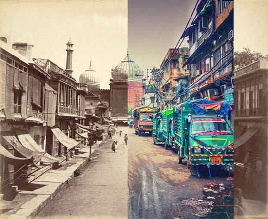
Figure 3.
The evolution of space around Jama Masjid from 1880s till present; source: ASI archive.

Figure 4.
Pipeline for generating the present and the past model of 2020s.

Figure 5.
Location of the buildings which were selected for collecting heights. The numbers represent the individual buildings and the alphabets contains multiple structures/buildings which are further zoomed in on the left.
Figure 5.
Location of the buildings which were selected for collecting heights. The numbers represent the individual buildings and the alphabets contains multiple structures/buildings which are further zoomed in on the left.

Figure 6.
Pleiades tri-stereo and Worldview-1 stereo pairs for DSM.

Figure 7.
Process involved in generating a DSM through stereo-based matching.

Figure 8.
Network architecture of ResDepth, authors: Corinne Stucker and Konrad Schindler [16].
Figure 8.
Network architecture of ResDepth, authors: Corinne Stucker and Konrad Schindler [16].

Figure 9.
(a) Conventionally obtained DSM; (b) output from ResDepth: the figure illustrates that the model fails to refine building structures, but the streets were widened, and much of the noise was removed.
Figure 9.
(a) Conventionally obtained DSM; (b) output from ResDepth: the figure illustrates that the model fails to refine building structures, but the streets were widened, and much of the noise was removed.

Figure 10.
Very dense point cloud created from images collected using Google Earth Pro.

Figure 11.
Shahjahanabad in 1977, captured by the KH-9 satellite: (a) Shahjahanabad cropped from the full strip; (b) area of interest with 70 cm GSD.
Figure 11.
Shahjahanabad in 1977, captured by the KH-9 satellite: (a) Shahjahanabad cropped from the full strip; (b) area of interest with 70 cm GSD.

Figure 12.
Cleaned film strips obtained after stitching and removing borders.

Figure 13.
The steps involved in generating the camera models and bundle adjustment for KH-9 images.
Figure 13.
The steps involved in generating the camera models and bundle adjustment for KH-9 images.

Figure 14.
Visual comparison of three DSMs for Jama Masjid mosque. The three domes with the minarets can be seen in the combined DSM, which the other two DSMs could not detect.
Figure 14.
Visual comparison of three DSMs for Jama Masjid mosque. The three domes with the minarets can be seen in the combined DSM, which the other two DSMs could not detect.

Figure 15.
Output DSM generated from all five images combined after rasterizing the point cloud.

Figure 16.
Output DSM generated from the stereo pairs of the KH-9 images.

Figure 17.
The numbers (right image) represent the selected ground control points for accuracy assessment; left: KH-9 image; right: extracted DTM of the 1970s.
Figure 17.
The numbers (right image) represent the selected ground control points for accuracy assessment; left: KH-9 image; right: extracted DTM of the 1970s.

Figure 18.
Illustration explaining the method used for accuracy assessment for the 1970s raster from the 2020s raster.
Figure 18.
Illustration explaining the method used for accuracy assessment for the 1970s raster from the 2020s raster.

Figure 19.
Final form of the rendered present city model of the 2020s.

Figure 20.
Final form of the rendered past city model of the 1970s.

Figure 21.
Bar graph showing the changes in the building counts from the 1970s to the 2020s.

Figure 22.
Classified height maps of the 2020s (a) and 1970s (b) showing the vertical expansion in the area; source: ArcGIS Pro.
Figure 22.
Classified height maps of the 2020s (a) and 1970s (b) showing the vertical expansion in the area; source: ArcGIS Pro.

Figure 23.
Visibility comparison of point A in the two models.

Figure 24.
Visibility comparison of point B in the two models.

Figure 25.
Visibility comparison of point C in the two models.

Figure 26.
Visibility comparison of point D in the two models.

Figure 27.
Results from drone-shot videos; (a) point cloud from Sfm; (b) obtained 3D model.

Figure 28.
Examples of some colorized rare photographs from late 19th century. Examples of some rare photographs from late 19th century, colorized through the DeOldify noGAN method [28].
Figure 28.
Examples of some colorized rare photographs from late 19th century. Examples of some rare photographs from late 19th century, colorized through the DeOldify noGAN method [28].


Table 1.
Metadata of the satellite images used for DSM creation.
| No. | Data | Date | GSD | Provider | Remarks | Used in |
|---|---|---|---|---|---|---|
| 1 | Pleiades Tri-Stereo VHR | 18 December 2020 | 0.5 m | ESA | PANSHARP | Present |
| 2 | Worldview-1 Stereo VHR | 19 March 2021 | 0.58 m | ESA | PAN | Present |
| 3 | Worldview-3 VHR | 7 February 2022 | 0.3 m | ESA | MUL 8-Bands | Present |
| 4 | Building footprints | 2018 | - | SPA | .shp file | Present |
| 5 | Hexagon KH-9 Stereo pair | 4 December 1977 | 0.7 m | USGS | Scanned B/W | Past |
| 6 | Building footprints | 1977 | - | Self-digitized | .shp file | Past |
Table 2.
Accuracy assessment of the three digital surface models.
| No. | Description | Ground Ref (m) | WV-1 DSM (m) | PL DSM (m) | Combined (m) |
|---|---|---|---|---|---|
| 1 | Red Fort: Front Centre | 34.0 | 39.97 | 35.7 | 32.0 |
| 2 | Red Fort Walls | 20.6 | 24.04 | 22.36 | 19.52 |
| 3 | Battlement | 12.6 | 16.45 | 14.67 | 12.54 |
| 4 | Jama Masjid, Main Gate 2, opp. domes | 14.0 | 18.48 | 12.68 | 13.74 |
| 5 | Jama Masjid, Corridor Roof | 5.8 | 7.32 | 7.83 | 5.59 |
| 6 | Fatehpuri Masjid, inside the entrance | 13.0 | 17.79 | 15.52 | 11.48 |
| 7 | SBI Building | 20.1 | 23.46 | 23.87 | 21.34 |
| 8 | Shri Gauri Shankar Mandir | 25.0 | 32.84 | 27.91 | 25.52 |
| 9 | Shri Digambar Jain Lal Mandir, side dome | 19.4 | 16.0 | 22.8 | 21.13 |
| 10 | Shri Digambar Jain Lal Mandir, main dome | 21.2 | 43.24 | 23.26 | 26.07 |
| 11 | Town Hall Library | 13.6 | 14.7 | 13.03 | 12.72 |
| 12 | MCD Civic Centre | 100.8 | 108.52 | 104.2 | 97.68 |
| 13 | TRAI Building | 32.1 | 39.81 | 30.2 | 32.96 |
| 14 | Zakir Hussain, Delhi University | 28.3 | 30.53 | 31.42 | 27.74 |
| 15 | Government of India, Press | 32.6 | 34.68 | 30.07 | 31.83 |
| 16 | Konnectus Tower | 36.2 | 41.74 | 42.21 | 39.55 |
| 17 | Common building 17 | 11.9 | 18.54 | 13.4 | 16.03 |
| 18 | Common building 18 | 10.6 | 14.09 | 9.18 | 14.89 |
| 19 | Common building 19 | 10.81 | 9.17 | 12.3 | 11.97 |
| 20 | Common building 20 | 11.8 | 8.23 | 10.97 | 11.88 |
| 21 | Common building 21 | 15.65 | 18.92 | 16.47 | 16.62 |
| RMSE | 6.62 | 2.55 | 2.15 m |
Table 3.
Accuracy assessment of the digital terrain model of the 1970s.
| GCP | Present DTM (m) | 1970s DTM (m) | Error (m) |
|---|---|---|---|
| 1 | 160.70 | 160.29 | −0.40 |
| 2 | 161.11 | 163.77 | −2.34 |
| 3 | 166.34 | 165.32 | −0.96 |
| 4 | 159.62 | 160.0 | 0.42 |
| 5 | 162.80 | 161.43 | −1.22 |
| 6 | 163.0 | 164.13 | 1.07 |
| 7 | 165.5 | 165.24 | −0.31 |
| 8 | 164.0 | 165.40 | 1.37 |
| 9 | 163.55 | 165.32 | 1.87 |
| 10 | 166.19 | 165.16 | −1.03 |
| RMSE | 1.25 + 2.15 (present DTM) = 3.40 m |
Table 4.
Table showing percentagewise increase and decrease in the building counts from the 1970s to 2020s.
Table 4.
Table showing percentagewise increase and decrease in the building counts from the 1970s to 2020s.
| Range in Meters | Building Count—1970s | Building Count—2020s | % Increase | % Decrease |
|---|---|---|---|---|
| 1 to 4 | 116 | 133 | 12.7% | |
| 4 to 8 | 872 | 86 | 90.1% | |
| 8 to 12 | 853 | 772 | 9.4% | |
| 12 to 16 | 146 | 2293 | 93.6% | |
| 16 to 20 | 12 | 1694 | 99.2% | |
| 20 to 24 | 0 | 514 | 100% | |
| 24 to 28 | 0 | 39 | 100% | |
| Avg Increase 81.1% | Avg Decrease 49.8% |
Table 5.
Table showing the percentagewise reduction in visibility of the targets from the chosen observation points.
Table 5.
Table showing the percentagewise reduction in visibility of the targets from the chosen observation points.
| Observation Point | No. of Targets | Visible in 1977 | Visible in 2022 | Visibility Reduction |
|---|---|---|---|---|
| A | 7 | 2 (28.5%) | 1 (14.2%) | 14.3% |
| B | 10 | 6 (60%) | 6 (60%) | 0% |
| C | 6 | 4 (66.6%) | 1 (16.6%) | 50% |
| D | 8 | 3 (37.5%) | 1 (12.5%) | 25% |
Disclaimer/Publisher’s Note: The statements, opinions and data contained in all publications are solely those of the individual author(s) and contributor(s) and not of MDPI and/or the editor(s). MDPI and/or the editor(s) disclaim responsibility for any injury to people or property resulting from any ideas, methods, instructions or products referred to in the content. |
© 2023 by the authors. Licensee MDPI, Basel, Switzerland. This article is an open access article distributed under the terms and conditions of the Creative Commons Attribution (CC BY) license (https://creativecommons.org/licenses/by/4.0/).
Share and Cite
MDPI and ACS Style
Rajan, V.; Koeva, M.; Kuffer, M.; Da Silva Mano, A.; Mishra, S. Three-Dimensional Modelling of Past and Present Shahjahanabad through Multi-Temporal Remotely Sensed Data. Remote Sens. 2023, 15, 2924. https://doi.org/10.3390/rs15112924
AMA Style
Rajan V, Koeva M, Kuffer M, Da Silva Mano A, Mishra S. Three-Dimensional Modelling of Past and Present Shahjahanabad through Multi-Temporal Remotely Sensed Data. Remote Sensing. 2023; 15(11):2924. https://doi.org/10.3390/rs15112924
Chicago/Turabian StyleRajan, Vaibhav, Mila Koeva, Monika Kuffer, Andre Da Silva Mano, and Shubham Mishra. 2023. "Three-Dimensional Modelling of Past and Present Shahjahanabad through Multi-Temporal Remotely Sensed Data" Remote Sensing 15, no. 11: 2924. https://doi.org/10.3390/rs15112924
Note that from the first issue of 2016, this journal uses article numbers instead of page numbers. See further details here.