
Study of a Steady-State Landscape Using Remote Sensing and Topographic Analysis
by
 , , ,
, , ,
Xueliang Wang
1,2,3,*,
Yanjie Zhang
4,
John J. Clague
5 ,
,
Songfeng Guo
1,2,3,
Qisong Jiao
6,
Junfei Wang
1,
Juanjuan Sun
1,2,3,
Wenxin Fang
1 and
Shengwen Qi
1,2,3 1
Key Laboratory of Shale Gas and Geoengineering, Institute of Geology and Geophysics, Chinese Academy of Sciences, Beijing 100029, China
2
Innovation Academy for Earth Sciences, CAS, Beijing 100029, China
3
College of Earth and Planetary Sciences, University of Chinese Academy of Sciences, Beijing 100049, China
4
Yunnan Dianzhong Water Diversion Engineering Co., Ltd., Kunming 650000, China
5
Department of Earth Sciences, Simon Fraser University, Burnaby, BC V5A 1S6, Canada
6
National Institute of Natural Hazards, MEMC, Beijing 100085, China
*
Author to whom correspondence should be addressed.
Remote Sens. 2023, 15(10), 2583; https://doi.org/10.3390/rs15102583
Submission received: 5 April 2023
/
Revised: 10 May 2023
/
Accepted: 12 May 2023
/
Published: 15 May 2023
(This article belongs to the Special Issue Ground Deformation Detection and Geomatic Applications by InSAR and GNSS Techniques II)
Abstract
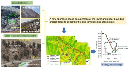
:The current limited approaches to calculating hillslope erosion rate hamper the study of the relationships among the rates of hillslope erosion, river incision, and tectonic uplift and hence the discussion of steady-state landscape evolution. In this paper, we use remote sensing and geochronological methods to calculate the upper and lower bounding hillslope erosion rates in the Qilian Shan range, Tibet. Our analysis focuses on five convex landslide sediment units derived from the weathered hillslopes at Qingyang Mountain on the tectonically active northeastern Tibetan Plateau. These sediment units range in thickness from 5.5 to 12.8 m and in volume from 119 × 103 to 260 × 103 m3. Based on field observations, measurements extracted from high-resolution DEMs, and optical stimulated luminescence (OSL) ages on fluvial terraces, we obtain lower and upper bounding rates of 0.13 ± 0.03 and 0.21 ± 0.04 mm/yr, respectively. Finally, we calculate incision rates, ranging from 0.21 ± 0.02 to 0.39 ± 0.01 mm/yr, from heights of a dated fluvial terrace above the present river and the time of abandonment of the associated bedrock strath estimated from OSL ages. The rates of hillslope erosion and river incision at Qingyang Mountain and the tectonic uplift of the Qilian Mountains are estimated to be within a factor of two over the past 117 ka, suggesting that a state of dynamic equilibrium has likely existed on this timescale.
1. Introduction
There is considerable interest among researchers in mountain landscape evolution on large spatial scales and over long temporal timescales [1,2,3,4,5,6]. It has been argued that similar hillslope gradients in different mountain ranges imply the development of threshold topography even under different rates of uplift and river incision [7,8,9]. Specifically, it is thought that hillslope angles in tectonically active landscapes remain constant (i.e., at a “threshold angle”) in terms of uplift and incision progress, with, for example, modal values of 31–39° in the northwestern Himalayas, southeastern Tibet, and other tectonically active ranges [7,8,9,10,11,12,13]. These results imply that hillslopes are strongly coupled with uplift and river incision, at least on long timescales [14].
Although a steady state is thought to be difficult to achieve in natural landscapes, a dynamic equilibrium over limited spatial and temporal scales (e.g., 106 yr) has been inferred in some mountains [10,15,16]. A topography in dynamic equilibrium requires a continuous adjustment of hillslope form to river incision [14]. Previous researchers have suggested that the rates of hillslope erosion, river incision, and rock uplift in active mountain ranges differ by roughly a factor of two ([15], northern Alpennines), but additional data from a variety of mountain ranges are required to verify and extend this conclusion. However, few studies using a quantitative approach have been carried out to provide such data [17].
Because the long-term rates of hillslope erosion are difficult to directly calculate, we propose an approach based on determining the lower and upper bounding values of the hillslope erosion rate on a long timescale in the Qilian Shan range, Tibet, based on remote sensing and topographic analysis. The context for our work is provided by previous studies that show that the use of satellite data, remote sensing techniques, and geological data enables accurate automated landslide identification [18], landslide monitoring [19], and landslide susceptibility mapping [20]. The analysis of the landscape in our study area is based, in part, on a high-resolution digital elevation model (DEM) created from aerial photographs obtained using an unmanned aerial vehicle (UAV) and processed using the structure-from-motion photogrammetric technique. We conducted a targeted field program at Qingyang Mountain (QYM) on the northeastern Tibetan Plateau (Figure 1) to determine the hillslope erosion and river incision rates based on a quantitative upper/lower boundary approach. Our objective is to contribute to discussions of if and how active mountain landscapes evolve toward a state of dynamic equilibrium.
2. Study Area
Our study area was located in the northeastern Qilian Shan range at the margin of the Tibetan Plateau (Figure 1). The range comprises Paleozoic volcanic and metasedimentary rocks, Caledonian granites, and Neogene sedimentary rocks [21]. The contemporary and Cenozoic tectonic environment is dominated by the convergence of the Indian and Eurasian plates, accompanied by folding, thrust faulting, and strike-slip faulting [22,23]. Deformation between the Qaidam and Alashan blocks is distributed throughout the ~270-km-wide Qilian Shan plateau and is accompanied by shortening at a rate of 5.5 (±1.5) mm/yr [24,25]. The Haiyuan fault, a major left-lateral strike-slip fault with an average Holocene slip rate of 4.5 ± 0.5 mm/yr, crosses Qilian Shan ~10 km south of our study area [26,27]. Several authors have presented evidence for late Pleistocene–Holocene vertical slip on thrust faults in the study area as follows: 0.4–1.9 mm/yr for the vertical uplift of Yumu shan [22]; 0.6–0.9 mm/yr for the Zhangye thrust [21]; 0.35 ± 0.05 mm/yr for the Yumen thrust [23]; 1.3 ± 0.2 mm/a in the southwestern Heli Shan [28]; 0.54–0.80 mm/yr for the Huangcheng–Taerzhuang fault [29]; 0.18–0.2 mm/a for the western segment, 0.3–0.43 mm/a for the central segment, and 0.36–0.53 mm/a for the eastern segment of the north side of Heli Shan thrust fault; and 0.21 mm/a for the Wutongjing Fault [30]. The mean annual temperature and mean annual precipitation (1956–2016) at QYM are 1.2 °C and 410 mm, respectively, with a July maximum in terms of precipitation [31]. We subdivided the QYM study area at elevations ranging from 3100 to 3600 m a.s.l. into three slopes with different aspects, which we refer to as the eastern QYM (facing 0–90°), southern QYM (facing 90–180°), and western QYM (facing 180–270°) areas. Three rivers border the eastern, southern, and western QYM, namely the Rixu (RX), Qingyang (QY), and Kuangqu (KQ) rivers, respectively (Figure 1b). RX and QY are perennial rivers, whereas KQ is a seasonal stream. In the eastern QYM, there are well-preserved terrace deposits and colluvial sediments on a bedrock strath, which provided us an opportunity to constrain the ages of the sediments and river incision.
Due to long-term weathering, permafrost activity, and extensive fracturing of the rock mass, there are frequent landslides on QYM. Hence, colluvium has progressively accumulated on the bedrock strath at the toes of the hillslopes and in gullies eroded into hillslopes. We identified five convex landslide sediment units (Figure 1b and Figure 2) derived from the weathered hillslopes on a single bedrock strath. The sediments include slopewash and very small (<0.001 m3) to small (0.001–0.04 m3) rock blocks [32]. The cover-eroded sediments have a total thickness of 5.5–12.8 m and volumes ranging from 119 × 103 to 260 × 103 m3. The cover sediments can be traced upslope to three gullies that terminate at the slope toes and have average depths ranging from 19.2 to 22.8 m. A fourth gulley, adjacent to the terrace, has an average depth of 13.9 m but is filled with eroded hillslope sediments.
3. Methods
3.1. Creating a Digital Elevation Model
Sparse vegetation of trees and bushes at QYM (Figure 2), especially in winter, allowed us to produce an accurate bare-earth DEM from UAV airphotos using structure-from-motion photogrammetry [33]. We obtained 476 photographs with a Phantom 4 RTK UAV over an area of about 10 km2 on 23 October 2020 when the ground surface was bare. The UAV provided real-time, centimeter-scale positioning data (https://www.dji.com/cn/phantom-4-rtk, (accessed on 11 May 2023)). A minimum of six ground control points (GCPs) were used at each site for geometrical positioning during the UAV survey. When applying the single-base-station measurement method, the points for GCPs are generally chosen as the intersection of linear objects with small elevation differences, as well as the centers of point-like objects. The reference coordinate system WGS84 was chosen for the measurement of the GCPs. The instrument had to be shut down and initialized before observation on site. The number of automatic observations per measurement was kept at no less than 30, and the average value was taken as the result. The accuracy threshold for each measuring point was H ≤ 2 cm in the horizontal plane and V ≤ 3 cm in the vertical direction. The flight height and velocity were calculated automatically. The lateral overlap of the photographs was more than 65%, and the heading overlap was more than 75% [34].
The 476 photographs were aligned to generate a DEM with a spatial resolution of 7 cm in AgiSoft Photoscan Version 1.2.6 (AgiSoft LLC, 2010, Petersburg, Russia). The structure-from-motion algorithm was used to derive the DEM data from the aerial images and involved feature point extraction, image matching, and bundle adjustments [33]. Photoscan adds and aligns photos, imports GCP coordinates, optimizes camera alignment, and builds a dense point cloud [34]. During the process, built-in filtering algorithms sort out outliers in the point cloud. We implemented a high accuracy, a key point limit of 40,000, aggressive depth filtering, and an arbitrary surface type in Photoscan. We sub-sampled the point cloud to a minimum point spacing of 0.3 m. The DEM was constructed from the point cloud by fitting polygons to points [33].
3.2. Estimating River Incision Rates
The RX River is bordered by a well-preserved bedrock strath covered by ~1.5–2.7 m of fluvial gravel and minor sand (Figure 3). We determined heights of the strath above the river using a laser range finder (vertical precision <0.1 m) and estimated its formative ages based on optical stimulated luminescence (OSL) ages on its sediment cover. In the following, the terrace heights are referred to as the bedrock strath and the modern river.
We estimated the time of the fluvial terrace abandonment by dating five samples of quartz sand from the fluvial cover unit (OSL-03 to OSL-08; Figure 1b) and two samples of quartz sand from the colluvium on the terrace (OSL-01 to OSL-02) using the OSL method [3]. OSL samples were collected at depths of 1.0–2.3 m below the ground surface by driving stainless-steel tubes (~5 cm inner diameter, ~25 cm long) horizontally into cleaned exposures of the terrace sediments. When the sediment-filled tubes were extracted from the exposures, the ends were immediately covered with aluminum foil and opaque tape to prevent exposure to sunlight.
OSL samples were dated at the Luminescence Dating Laboratory of the Institute of Geology, China Earthquake Administration (Table 1). The sensitivity-corrected multiple-aliquot regenerative-dose protocol for OSL was used to calculate the equivalent dose (De) values for the samples [3]. Multiple aliquots of quartz grains (4–11 μm) were used to build the OSL growth curve.
3.3. Estimating Hillslope Erosion Rates
The QYM hillslopes are currently experiencing erosion, but determining the long-term rates of erosion there, or for that matter anywhere, is difficult due to the limited evidence and approaches [36]. We propose an approach to determine the lower and upper bounding rates of hillslope erosion in the eastern QYM. First, when a strath is abandoned due to incision by a trunk stream, it becomes a terrace on which slopewash and landslide sediments derived from the adjacent higher hillslope begin to accumulate. We estimated the total amount of material eroded from the hillslope by determining the volume of colluvium lying on the terrace. We considered the rate of landslide erosion calculated in this way to be the lower bounding value because some of the sediment deposited on the terrace had likely been lost due to fluvial erosion. We calculated this lower bounding rate (Eh-l) by dividing today’s total volume (Vd) of colluvium on the terrace by the horizontal surface area of the landslide source (As) and the time over which the erosion occurred (TL) [36]:
We assumed TL to be the time since the fluvial terrace abandonment, as determined from the OSL ages. The colluvium derived from hillslope erosion was identified on our 0.3 m resolution DEM and checked in the field (Figure 4). To estimate total volume (Vd), we calculated the geometric parameters of the landslide deposit, including the deposit horizontal surface area (Ad) and average thickness (Dd). We estimated the deposit thickness (Dd) and confirmed the hillslope sources in the field. We then mapped the deposits and hillslope source areas from orthophotos and the DEM in ArcMAP to obtain their horizontal surface areas (Ad and As, respectively) (Figure 2 and Figure 5). The deposit volume (Vd) was calculated as the product of the horizontal surface area and the average thickness of the deposit (Vd = Ad × Dd).
It was difficult to delineate the exact boundaries of the historic landslides from the imagery. However, based on the field investigation, we inferred that some sections of the terrace in the eastern QYM was destroyed by historic landslides and hence the colluvium identified in the field (Figure 4) was deposited after the fluvial terrace formed. We calculated the ratio (α) of the channel width (W) to the channel depth (D) of the existing, non-destroyed strath terrace to estimate the initial width of the fluvial terrace that was subsequently eroded and covered by colluvium. The colluvial cover on the terrace was likely a product of recurrent slopewash and rockfall processes, which are related to rock weathering and movement from the source area.
An upper bounding estimate of the hillslope erosion rate was obtained from the slope gullies. Over time, flat hillslopes become gullied, especially on slopes with highly fractured rock. If we know how long a hillslope has been eroding (time) and how far back the slope has eroded (depth) before the gullies formed, we can estimate the hillslope erosion rate (depth/time). However, it is difficult to determine the initial time of the gully erosion. In the case of the eastern QYM hillslope, the time that the gullies began to form was probably earlier than the time the river abandoned the level of the fluvial terrace due to the incision of the bedrock strath. We thus inferred that the current gullies were created in two stages: first, before the fluvial terrace formed, and, later, after the terrace surface was abandoned. Hence, the volume of the source sediment calculated based on gulley depths must be too large because the gullies could have formed over a period before the terrace was abandoned. We therefore regarded the hillslope erosion rates based on these depths to be the rough upper bounding rates in this study.
Accepting this assumption, we could calculate an upper-bound hillslope erosion rate (Eh-u) by dividing the average gulley depth (i.e., erosion depth) by the fluvial terrace abandonment time. We determined the average gully depth (H) by differencing the maximum and minimum elevations of gulley cross-sections (Hi, i from 1 to n) separated by 1 m along the hillslope (i.e., the resolution of the DEM created from sub-sampled point clouds) using the equation of H = (H1 + H2 + …+ Hn)/n (Figure 6). In our study of the eastern QYM, n ranged from 262 to 512. The time of terrace abandonment (TL) was assumed to be the same as that calculated in Equation (2).
4. Results
4.1. Initial Boundary of Fluvial Terrace
We calculated the ratio (α) of the channel width (W) to the channel depth (D) by extracting data from the bedrock channels of the eastern QYM, where paleo-channels are not covered by hillslope erosion deposits. Significant linear relations between W and D were apparent in these channels (Figure 7a), with an average α value of 4.6 ± 1.2. Using the calculated average α value and the value of D for the well-preserved bedrock channels, we estimated the initial channel width of the fluvial terrace (Figure 7b). The comparison of the estimated initial and current boundaries of the deposits eroded from the slope helped us to identify the locations of the ends of the eroded gullies (U01–U04 in Figure 5 and Figure 7b) and thus to estimate the hillslope erosion rate.
4.2. River Incision Rates
Two samples of colluvial sediments (samples of OSL-01 and OSL-02) yielded OSL ages of 32.79 ± 0.89 ka and 44.70 ± 1.25 ka (Table 1), respectively. The other six OSL samples (OSL-03 to OSL-08) were collected from sand lenses within the capping fluvial terrace gravel and yielded ages of 89.92 ± 6.9, 93.83 ± 3.34, 117.04 ± 4.63, 73.33 ± 4.41, 80.90 ± 5.2, and 72.58 ± 2.16 ka, respectively. Five of these samples (OSL-04 to OSL-08) were collected from similar heights above the river (27.5–29.5 m). We inferred that these sediments could date the time of the abandonment of the bedrock strath.

Table 1.
Estimates of incision rate based on abandonment ages of bedrock strath in QYM.
| Field Sample ID | Latitude North (deg) | Longitude East (deg) | Sample Depth (m) | Equivalent Dose (σ) Gy | Dose Rate (σ) Gy/ka | OSL Age (σ) ka | Height of Terrace (σ) m | Incision Rate (σ) mm/yr |
|---|---|---|---|---|---|---|---|---|
| OSL-01 | 38.169 | 100.438 | 2.3 | 126.81 (1.10) | 3.87 (0.10) | 32.79 (0.89) | 12.5 (0.1) | 0.38 (0.01) |
| OSL-02 | 38.169 | 100.437 | 1.4 | 162.44 (1.79) | 3.63 (0.09) | 44.70 (1.25) | 13.0 (0.1) | 0.29 (0.01) |
| OSL-03 | 38.169 | 100.437 | 1.0 | 396.35 (19.67) | 4.41 (0.26) | 89.92 (6.9) | 18.5 (0.1) | 0.21 (0.02) |
| OSL-04 | 38.175 | 100.431 | 2.2 | 351.01 (7.91) | 3.74 (0.10) | 93.83 (3.34) | 29.5 (0.1) | 0.31 (0.01) |
| OSL-05 | 38.175 | 100.431 | 2.3 | 401.67 (11.11) | 3.43 (0.10) | 117.04 (4.63) | 29.0 (0.1) | 0.25 (0.01) |
| OSL-06 | 38.176 | 100.430 | 1.5 | 324.1 (11.18) | 4.42 (0.22) | 73.33 (4.41) | 28.0 0.1) | 0.38 (0.02) |
| OSL-07 | 38.176 | 100.430 | 1.1 | 388.97 (3.25) | 4.81 (0.26) | 80.90 (5.20) | 27.5 0.1) | 0.34 (0.02) |
| OSL-08 | 38.176 | 100.430 | 1.6 | 240.01 (3.33) | 3.31 (0.09) | 72.58 (2.16) | 28.0 (0.1) | 0.39 (0.01) |
We calculated the incision rate (Table 1) at each sample site from the abandonment age of the fluvial terrace and the height of the bedrock strath surface above the modern river using Equation (1). Uncertainties in the calculated incision rates were mainly sourced from uncertainties in the estimated terrace abandonment ages. The dated abandonment ages used in Equation (1) were the upper limits based on the fluvial sediment cover on the bedrock strath. However, given the estimates of the modern incision rates of tens of mm/yr in eastern Tian Shan, several hundred kilometers from our study area, by [17], the time required for the fluvial deposits covering the bedrock strath to become incised and thus fossilized were within the uncertainties of the OSL ages (σ from 0.89 to 5.20 ka).
All incision rates were calculated based on the time elapsed since the assumed time of the terrace abandonment (Table 1). In conclusion, we estimated the rates of river incision in the eastern QYM to be in the range from 0.21 ± 0.02 to 0.39 ± 0.01 mm/yr. These values were broadly similar to estimates of incision rates in the eastern Qilian Shan range (0.32–0.62 mm/yr) over the past 1.4 Ma [21].
4.3. Hillslope Erosion Rates
We calculated the volumes of the hillslope erosion products and source-scar areas at five sites in QYM (L01–L05 in Figure 5). The deposits at the five sites covered the fluvial terrace and were up to 12.8 m thick. Based on the estimated OSL ages for strath abandonment, we assumed that hillslope erosion began after 117.04 ka (Tlower) and possibly after 72.58 ka (Tupper). Using Equation (2), we established a lower bound of the hillslope erosion rates in the eastern QYM ranging from 0.09 to 0.20 mm/yr (Table 2), with an average value of 0.13 ± 0.03 mm/yr.
Table 2.
Measured geometric parameters of erosion deposits (area of deposits Ad, depth of deposits Dd, and deposit volume Vd); source area (As); and calculated minimum and maximum lower bounding hillslope erosion rates based on upper and lower ages of dated fluvial terrace abandonment.
Table 2.
Measured geometric parameters of erosion deposits (area of deposits Ad, depth of deposits Dd, and deposit volume Vd); source area (As); and calculated minimum and maximum lower bounding hillslope erosion rates based on upper and lower ages of dated fluvial terrace abandonment.
| No. | Ad (m2) | Dd (m) | Vd (m3) | As (m2) | Erosion Depth (m) | Min. of Eh-l (mm/yr) | Max. of Eh-l (mm/yr) |
|---|---|---|---|---|---|---|---|
| L01 | 20,679 | 11.4 | 235,743 | 18,225 | 12.9 | 0.11 | 0.18 |
| L02 | 21,608 | 5.5 | 118,848 | 15,448 | 7.7 | 0.07 | 0.11 |
| L03 | 22,414 | 11.6 | 260,004 | 17,582 | 14.8 | 0.13 | 0.20 |
| L04 | 21,426 | 7.3 | 156,413 | 15,417 | 10.2 | 0.09 | 0.14 |
| L05 | 15,106 | 12.8 | 193,359 | 17,627 | 11.0 | 0.09 | 0.15 |
Note: Max. of Eh-l was calculated by dividing erosion depth by Tupper. Min. of Eh-l was calculated by dividing erosion depth by Tlower. Tupper and Tlower were 72.58 and 117.04 ka, respectively.
The average depths of the four gullies (U01–U04 in Figure 5) were from 13.87 to 22.78 m. By dividing total average gully depth reduction values (da) by the assumed fluvial terrace abandonment ages of 72.58 ka (Tupper) and 117.04 ka (Tlower), we arrived at the upper hillslope erosion rates (Eh-u) of 0.12–0.31 mm/yr (Table 3), with an average of 0.21 ± 0.04 mm/yr.
Table 3.
Measured depth-reduction values of eroded gullies and calculated minimum and maximum upper hillslope erosion rates using upper and lower ages of fluvial terrace abandonment.
Table 3.
Measured depth-reduction values of eroded gullies and calculated minimum and maximum upper hillslope erosion rates using upper and lower ages of fluvial terrace abandonment.
| No. | Ave, Depth Reduction (da) (m) | Max. Eh-u (mm/yr) | Min. Eh-u (mm/yr) |
|---|---|---|---|
| U01 | 19.2 | 0.26 | 0.16 |
| U02 | 20.0 | 0.28 | 0.17 |
| U03 | 13.9 | 0.19 | 0.12 |
| U04 | 22.8 | 0.31 | 0.19 |
Note: Max. Eh-u was calculated by dividing the average gully depth by Tupper. Min. Eh-u was calculated by dividing the average depth by Tlower. Tupper and Tlower were 72.58 and 117.04 ka, respectively.
5. Discussion
It is difficult to distinguish erosion before a terrace is formed from the subsequent erosion. Therefore, we used the calculated average value of gully erosion as the upper bound for the hillslope erosion following terrace abandonment due to incision. The average hillslope erosion rate in the eastern QYM, assuming lower and upper bounding rates of 0.13 ± 0.03 and 0.21 ± 0.04 mm/yr, was 0.17 ± 0.04 mm/yr. This value was lower than our estimate of the average river incision rate of 0.32 ± 0.07 mm/yr over the past 117 ka. Both the hillslope and river incision rates were near the lower limit of published regional vertical uplift rates (0.18–1.90 mm/yr [21,29,30]). Because researchers have concluded that hillslope erosion rates, river incision, and rock uplift in other active mountain ranges differ by roughly a factor of two in a steady state (e.g., so-called ‘dynamic equilibrium’; [15]), we inferred that river incision and hillslope erosion in QYM have probably balanced the regional vertical uplift over the past ~0.1 Ma, which is within the range of one (~105 y) or more climate cycles [10]. Montgomery [14] observed that the Oregon Coast Range may be at steady state, but it does not have bedrock threshold hillslopes. Our study of QYM likely documents such an additional example. The time scale for hillslopes to adjust to changes in river incision in the northern Alpennines is thought to be ~0.1 My [15], which is similar to our estimate of the time of river incision at QYM (~117.04 ka). Hence, hillslope erosion, river incision, and tectonic uplift in QYM appear to be in equilibrium to within a range of 0.18–1.90 mm/yr (Figure 8).
We acknowledge that there is much uncertainty in our estimates of the volume of colluvium generated by hillslope erosion, especially in the values of average thickness (Dd). We also do not know the exact extent of the colluvial sediments when the strath terrace formed, although we can safely assume that most of the colluvium accumulated on the terrace after the strath was abandoned. We also do not know whether some sediment deposited on the terrace was removed by erosion, thus limiting our estimates of Dd. It is for these reasons that we view our hillslope erosion rates in QYM as minimum values. We note that previous studies demonstrate that the calculated river incision rates in eastern Qilian Shan range from 0.09 to 1.49 mm/a [21,37]. Although differences in incision rates are likely due, in part, to different rates of local rock uplift, our method provides a new way of estimating long-term incision rates in tectonically active mountain landscapes.
6. Conclusions
- Using remote sensing, topographic analysis, and field investigation, we identified five convex colluvial landforms at the base of weathered hillslopes at Qingyang Mountain with a total thickness of 5.5–12.8 m and volumes ranging from 119 × 103 to 260 × 103 m3. The colluvial sediments accumulated after a bedrock strath 27.5–29.5 m above the present river level was abandoned, i.e., sometime after 73.33 ± 4.41 to 117.04 ± 4.63 kyr ago.
- We proposed an approach based on estimates of the lower and upper bounding erosion rates to constrain the long-term hillslope erosion rate at Qingyang Mountain. Applying this approach, we estimated the average hillslope erosion rate in this part of the eastern QYM to be between 0.13 ± 0.03 and 0.21 ± 0.04 mm/yr (average of 0.17 ± 0.04 mm/yr).
- Considering the published regional uplift rates (0.18–1.90 mm/yr) and the calculated rates of river incision (0.32 ± 0.07 mm/yr) and hillslope erosion (0.17 ± 0.04 mm/yr) in QYM, we hypothesize that QYM has been in a steady state over at least the past 100 ka.
Author Contributions
Conceptualization, X.W.; methodology X.W., J.S. and J.W.; formal analysis, X.W., W.F. and J.S.; Investigation, X.W., J.S. and Q.J.; writing—original draft preparation, X.W., S.Q. and J.J.C.; writing—review and editing, X.W., J.J.C. and S.Q.; visualization, S.G. and Q.J.; supervision, S.Q. and J.J.C.; project administration, X.W. and S.Q.; funding acquisition, Y.Z. and S.Q. All authors have read and agreed to the published version of the manuscript.
Funding
This work was supported by the key science and technology special program of Yunnan province (no. 202002AF080003), the China Natural Science Foundation (grant no. 42172304), and the Second Tibetan Plateau Scientific Expedition and Research Program (STEP) (grant no. 2019QZKK0904).
Data Availability Statement
The data presented in this study are available on request from the corresponding author.
Acknowledgments
We thank Yong Zhang, Haiyang Liu, and Ran Wang for their help in the field work.
Conflicts of Interest
The authors declare no conflict of interest.
References
- Herman, F.; Seward, D.; Valla, P.G.; Carter, A.; Kohn, B.; Willett, S.D.; Ehlers, T.A. Worldwide acceleration of mountain erosion under a cooling climate. Nature 2013, 504, 423–426. [Google Scholar] [CrossRef] [PubMed]
- Val, P.; Venerdini, A.L.; Ouimet, W.; Alvarado, P.; Hoke, G.D. Tectonic control of erosion in the southern Central Andes. Earth Planet. Sci. Lett. 2018, 482, 160–170. [Google Scholar] [CrossRef]
- Zhang, J.; Liu-Zeng, J.; Scherler, D.; Yin, A.; Wang, W.; Tang, M.-Y.; Li, Z.-F. Spatiotemporal variation of late Quaternary river incision rates in southeast Tibet, constrained by dating fluvial terraces. Lithosphere 2018, 10, 662–675. [Google Scholar] [CrossRef]
- Adams, B.A.; Whipple, K.X.; Forte, A.M.; Heimsath, A.M.; Hodges, K.V. Climate controls on erosion in tectonically active landscapes. Sci. Adv. 2020, 6, eaaz3166. [Google Scholar] [CrossRef]
- Lan, H.; Peng, J.; Zhu, Y.; Li, L.; Pan, B.; Huang, Q.; Li, J.; Zhang, Q. Geological and surficial processes and major disaster effects in the Yellow River Basin. Sci. China Earth Sci. 2022, 65, 234–256. [Google Scholar] [CrossRef]
- Zhang, W.; Wang, J.; Chen, J.; Soltanian, M.R.; Dai, Z.; WoldeGabriel, G. Mass-wasting-inferred dramatic variability of 130,000-year Indian summer monsoon intensity from deposits in the southeast Tibetan Plateau. Geophys. Res. Lett. 2022, 49, e2021GL097301. [Google Scholar] [CrossRef]
- Burbank, D.W.; Leland, J.; Fielding, E.; Anderson, R.S.; Liu, N.; Reid, M.R.; Duncan, C. Bedrock incision, rock uplift and threshold hillslopes in the northwestern Himalayas. Nature 1996, 379, 505–510. [Google Scholar] [CrossRef]
- Montgomery, D.R.; Brandon, M.T. Topographic controls on erosion rates in tectonically active mountain ranges. Earth Planet. Sci. Lett. 2002, 201, 481–489. [Google Scholar] [CrossRef]
- Larsen, I.J.; Montgomery, D.R. Landslide erosion coupled to tectonics and river incision. Nat. Geosci. 2012, 5, 468–473. [Google Scholar] [CrossRef]
- Burbank, D.W. Rates of erosion and their implications for exhumation. Mineral. Mag. 2002, 66, 25–52. [Google Scholar] [CrossRef]
- Korup, O. Rock type leaves topographic signature in landslide-dominated mountain ranges. Geophys. Res. Lett. 2008, 35, L11402. [Google Scholar] [CrossRef]
- Ouimet, W.B.; Whipple, K.X.; Granger, D.E. Beyond threshold hillslopes: Channel adjustment to base-level fall in tectonically active mountain ranges. Geology 2009, 37, 579–582. [Google Scholar] [CrossRef]
- DiBiase, R.A.; Heimsath, A.M.; Whipple, K.X. Hillslope response to tectonic forcing in threshold landscapes. Earth Surf. Process. Landf. 2012, 37, 855–865. [Google Scholar] [CrossRef]
- Montgomery, D.R. Slope distributions, threshold hillslopes, and steady-state topography. Am. J. Sci. 2001, 301, 432–454. [Google Scholar] [CrossRef]
- Cyr, A.J.; Granger, D.E. Dynamic equilibrium among erosion, river incision, and coastal uplift in the northern and central Apennines, Italy. Geology 2008, 36, 103–106. [Google Scholar] [CrossRef]
- Zondervan, J.R.; Stokes, M.; Boulton, S.J.; Telfer, M.W.; Mather, A.E. Rock strength and structural controls on fluvial erodibility: Implications for drainage divide mobility in a collisional mountain belt. Earth Planet. Sci. Lett. 2020, 538, 116221. [Google Scholar] [CrossRef]
- Malatesta, L.C.; Avouac, J.P.; Brown, N.D.; Breitenbach, S.F.M.; Pan, J.W.; Chevalier, M.L.; Rhode, E.; Saint-Carlier, D.; Zhang, W.J.; Charreau, J.L.; et al. Lag and mixing during sediment transfer across the Tian Shan piedmont caused by climate-driven aggradation-incision cycles. Basin Res. 2018, 30, 613–635. [Google Scholar] [CrossRef]
- Liu, P.; Wei, Y.; Wang, Q.; Chen, Y.; Xie, J. Research on post-earthquake landslide extraction algorithm based on improved U-Net Model. Remote Sens. 2020, 12, 894. [Google Scholar] [CrossRef]
- Karagianni, A.; Lazos, I.; Chatzipetros, A. Remote sensing techniques in disaster management: Amynteon Mine landslides, Greece. In Intelligent Systems for Crisis Management; Lecture Notes in Geoinformation and Cartography; Springer International Publishing: Cham, Switzerland, 2019; pp. 209–235. [Google Scholar] [CrossRef]
- Kalantar, B.; Ueda, N.; Saeidi, V.; Ahmadi, K.; Halin, A.A.; Shabani, F. Landslide susceptibility mapping: Machine and ensemble learning based on remote sensing big data. Remote Sens. 2020, 12, 1737. [Google Scholar] [CrossRef]
- Pan, B.T.; Hu, X.F.; Gao, H.S.; Hu, Z.B.; Cao, B.; Geng, H.P.; Li, Q.Y. Late Quaternary river incision rates and rock uplift pattern of the eastern Qilian Shan Mountain, China. Geomorphology 2013, 184, 84–97. [Google Scholar] [CrossRef]
- Tapponnier, P.; Meyer, B.; Avouac, J.P.; Peltzer, G.; Gaudemer, Y.; Guo, S.M.; Xiang, H.F.; Yin, K.L.; Chen, Z.T.; Cai, S.H.; et al. Active thrusting and folding in the Qilian Shan, and decoupling between upper crust and mantle in northeastern Tibet. Earth Planet. Sci. Lett. 1990, 97, 382–403. [Google Scholar] [CrossRef]
- Hetzel, R.; Niedermann, S.; Tao, M.; Kubik, P.W.; Ivy-Ochs, S.; Gao, B.; Strecker, M.R. Low slip rates and long-term preservation of geomorphic features in Central Asia. Nature 2002, 417, 428–432. [Google Scholar] [CrossRef] [PubMed]
- Zhang, P.; Shen, Z.; Burgman, R.; Molnar, P.; Wang, Q.; Niu, Z.; Sun, J.; Wu, J.; Sun, H.; You, X. Continuous deformation of the Tibetan Plateau constrained from global positioning measurements. Geology 2004, 32, 809–812. [Google Scholar] [CrossRef]
- Yuan, D.; Zhang, P.; Liu, B.; Gan, W.; Mao, F.; Wang, Z.; Zheng, D.; Guo, H. Geometrical imagery and tectonic transformation of late Quaternary active tectonics in northeastern margin of Qinghai-Xizang Plateau. Acta Geol. Sin. 2004, 78, 270–278. [Google Scholar]
- Li, C.Y.; Zhang, P.Z.; Yin, J.H.; Min, W. Late Quaternary left-lateral slip rate of the Haiyuan fault, northeastern margin of the Tibetan Plateau. Tectonics 2009, 28, TC5010. [Google Scholar] [CrossRef]
- Ji, T.; Zheng, W.; Yang, J.; Zhang, D.; Liang, S.; Li, Y.; Liu, T.; Zhou, H.; Feng, C. Tectonic significances of the geomorphic evolution in the southern Alashan Block to the outward expansion of the northeastern Tibetan Plateau. Remote Sens. 2022, 14, 6269. [Google Scholar] [CrossRef]
- Hetzel, R.; Tao, M.-X.; Niedermann, S.; Strecker, M.R.; Ivy-Ochs, S.; Kubik, P.W.; Gao, B. Implications of the fault scaling law for the growth of topography: Mountain ranges in the broken foreland of NE Tibet. Terra Nova 2004, 16, 157–162. [Google Scholar] [CrossRef]
- Chen, W.B. Principal Features of Tectonic Deformation and Their Generation Mechanism in the Hexi Corridor and Its Adjacent Regions Since Late Quaternary; Institute of Geology, China Seismological Bureau: Beijing, China, 2003; pp. 32–55. (In Chinese) [Google Scholar]
- Zheng, W.J.; Zhang, P.Z.; Ge, W.P.; Molnar, P.; Zhang, H.P.; Yuan, D.Y.; Liu, J.H. Late Quaternary slip rate of the South Heli Shan Fault (northern Hexi Corridor, NW China) and its implications for northeastward growth of the Tibetan Plateau. Tectonics 2013, 32, 271–293. [Google Scholar] [CrossRef]
- Zhang, Y.; Stoffel, M.; Liang, E.Y.; Guillet, S.; Shao, X.M. Centennial-scale process activity in a complex landslide body in the Qilian Mountains, northeast Tibetan Plateau, China. Catena 2019, 179, 29–38. [Google Scholar] [CrossRef]
- ISRM. Suggested methods for the quantitative description of discontinuities in rock masses. Int. J. Rock Mech. Min. Sci. Geomech. Abstr. 1978, 15, 319–368. [Google Scholar] [CrossRef]
- Johnson, K.; Nissen, E.; Saripalli, S.; Arrowsmith, J.R.; McGarey, P.; Scharer, K.; Williams, P.; Blisniuk, K. Rapid mapping of ultrafine fault zone topography with structure from motion. Geosphere 2014, 10, 969–986. [Google Scholar] [CrossRef]
- Wang, X.L.; Crosta, G.B.; Clague, J.J.; Stead, D.; Sun, J.; Qi, S.; Liu, H. Fault controls on spatial variation of fracture density and rock mass strength within the Yarlung Tsangpo Fault damage zone (southeastern Tibet). Eng. Geol. 2021, 291, 106238. [Google Scholar] [CrossRef]
- Wegmann, K.W.; Pazzaglia, F.J. Late Quaternary fluvial terraces of the Romagna and Marche Apennines, Italy: Climatic, lithologic, and tectonic controls on terrace genesis in an active orogeny. Quat. Sci. Rev. 2009, 28, 37–165. [Google Scholar] [CrossRef]
- Malamud, B.D.; Turcotte, D.L.; Guzzetti, F.; Reichenbach, P. Landslides, earthquakes, and erosion. Earth Planet. Sci. Lett. 2004, 229, 45–59. [Google Scholar] [CrossRef]
- Pan, B.T.; Gao, H.S.; Wu, G.J.; Li, J.J.; Li, B.Y.; Ye, Y.G. Dating of erosion surface and terraces in the eastern Qilian Shan, northwest China. Earth Surf. Process. Landf. 2007, 32, 143–154. [Google Scholar] [CrossRef]
Figure 1.
(a) Geologic map of part of the northern Tibetan Plateau (modified from [21,30] and our interpretation). Tectonic uplift rates obtained by previous studies are presented (① [22]; ② [21]; ③ [30]; ④ [28]). (b) Hillshade map of QYM showing locations of eight samples collected for optical stimulated luminescence dating and deposits.

Figure 2.
Five colluvial deposits (Ae) and their hillslope sources (As) shown on a UAV-acquired orthophoto.
Figure 2.
Five colluvial deposits (Ae) and their hillslope sources (As) shown on a UAV-acquired orthophoto.

Figure 3.
(a) Bedrock strath overlain by fluvial gravel and colluvium derived from hillslope erosion in the eastern QYM area. (b) Photo (direction = ~120°) showing the contact between the bedrock strath and overlying fluvial gravel and the locations of OSL samples collected from the fluvial cover unit (OSL-04–OSL-08).

Figure 4.
Identification of hillslope sediments (i.e., landslide deposits) and hillslope sources (i.e., potential slope-failure sites).
Figure 4.
Identification of hillslope sediments (i.e., landslide deposits) and hillslope sources (i.e., potential slope-failure sites).

Figure 5.
Slope deposits (Ad) and hillslope sources (As) plotted on a slope angle map derived from the DEM. The inset illustrates geometrical properties based on a real topographic profile (I-I′). Estimates of bounding erosion rates are included in the legend at the left. Lower avg. erosion rates and upper avg. erosion rates are from Tables 2 and 3.

Figure 6.
(a) Sketch map for calculating average gully depth (H) by differencing maximum (Emax) and minimum (Emin) elevations of different gulley cross-sections with different colors in (b).
Figure 6.
(a) Sketch map for calculating average gully depth (H) by differencing maximum (Emax) and minimum (Emin) elevations of different gulley cross-sections with different colors in (b).

Figure 7.
(a) Relationship between river channel width and depth in eastern QYM. (b) Initial boundary of bedrock channel (black line) reconstructed from field measurements of preserved channels (red line) and calculation of the ratio of width to depth (α).
Figure 7.
(a) Relationship between river channel width and depth in eastern QYM. (b) Initial boundary of bedrock channel (black line) reconstructed from field measurements of preserved channels (red line) and calculation of the ratio of width to depth (α).

Figure 8.
Inferred pattern of hillslope evolution in eastern QYM controlled by river incision. Colored lines include the minimum (green line), average (black line), and maximum (red line) profiles. Rock uplift rate is averaged from previous studies [21,23,26,29,30]. Rates of river incision and hillslope erosion were estimated in this study.

Disclaimer/Publisher’s Note: The statements, opinions and data contained in all publications are solely those of the individual author(s) and contributor(s) and not of MDPI and/or the editor(s). MDPI and/or the editor(s) disclaim responsibility for any injury to people or property resulting from any ideas, methods, instructions or products referred to in the content. |
© 2023 by the authors. Licensee MDPI, Basel, Switzerland. This article is an open access article distributed under the terms and conditions of the Creative Commons Attribution (CC BY) license (https://creativecommons.org/licenses/by/4.0/).
Share and Cite
MDPI and ACS Style
Wang, X.; Zhang, Y.; Clague, J.J.; Guo, S.; Jiao, Q.; Wang, J.; Sun, J.; Fang, W.; Qi, S. Study of a Steady-State Landscape Using Remote Sensing and Topographic Analysis. Remote Sens. 2023, 15, 2583. https://doi.org/10.3390/rs15102583
AMA Style
Wang X, Zhang Y, Clague JJ, Guo S, Jiao Q, Wang J, Sun J, Fang W, Qi S. Study of a Steady-State Landscape Using Remote Sensing and Topographic Analysis. Remote Sensing. 2023; 15(10):2583. https://doi.org/10.3390/rs15102583
Chicago/Turabian StyleWang, Xueliang, Yanjie Zhang, John J. Clague, Songfeng Guo, Qisong Jiao, Junfei Wang, Juanjuan Sun, Wenxin Fang, and Shengwen Qi. 2023. "Study of a Steady-State Landscape Using Remote Sensing and Topographic Analysis" Remote Sensing 15, no. 10: 2583. https://doi.org/10.3390/rs15102583
Note that from the first issue of 2016, this journal uses article numbers instead of page numbers. See further details here.