

Comparison of Machine Learning Algorithms for Flood Susceptibility Mapping
by
 , , , and
Seyd Teymoor Seydi
1,
Yousef Kanani-Sadat
1,
Mahdi Hasanlou
1 ,
,
Roya Sahraei
1,
Jocelyn Chanussot
2,3 and
Meisam Amani
4,*
1
School of Surveying and Geospatial Engineering, College of Engineering, University of Tehran, Tehran 14174-66191, Iran
2
Aerospace Information Research Institute, Chinese Academy of Sciences, Beijing 100094, China
3
Grenoble INP, GIPSA-Lab, CNRS, University Grenoble Alpes, 38000 Grenoble, France
4
WSP Environment & Infrastructure Canada Limited, Ottawa, ON K2E 7L5, Canada
*
Author to whom correspondence should be addressed.
Remote Sens. 2023, 15(1), 192; https://doi.org/10.3390/rs15010192
Submission received: 8 November 2022
/
Revised: 20 December 2022
/
Accepted: 27 December 2022
/
Published: 29 December 2022
(This article belongs to the Special Issue Remote Sensing Applications in Flood Forecasting and Monitoring)
Abstract
:Floods are one of the most destructive natural disasters, causing financial and human losses every year. As a result, reliable Flood Susceptibility Mapping (FSM) is required for effective flood management and reducing its harmful effects. In this study, a new machine learning model based on the Cascade Forest Model (CFM) was developed for FSM. Satellite imagery, historical reports, and field data were used to determine flood-inundated areas. The database included 21 flood-conditioning factors obtained from different sources. The performance of the proposed CFM was evaluated over two study areas, and the results were compared with those of other six machine learning methods, including Support Vector Machine (SVM), Decision Tree (DT), Random Forest (RF), Deep Neural Network (DNN), Light Gradient Boosting Machine (LightGBM), Extreme Gradient Boosting (XGBoost), and Categorical Boosting (CatBoost). The result showed CFM produced the highest accuracy compared to other models over both study areas. The Overall Accuracy (AC), Kappa Coefficient (KC), and Area Under the Receiver Operating Characteristic Curve (AUC) of the proposed model were more than 95%, 0.8, 0.95, respectively. Most of these models recognized the southwestern part of the Karun basin, northern and northwestern regions of the Gorganrud basin as susceptible areas.
1. Introduction
Natural disasters such as landslides, wildfires, tsunamis, and floods cause huge financial and human losses every year [1,2,3]. The effects of flooding are detrimental to human and ecological wellbeing around the world, making it one of the most destructive disasters [4]. For example, according to statistics, floods are accountable for more than half of the damage caused by natural disasters over the last five decades [5,6,7]. There are many immediate impacts of flooding, including loss of life, damage to properties and infrastructure, as well as loss of crops and livestock. Although many efforts have been made to reduce the negative effects of floods, the number of flood events has considerably increased [8]. Thus, reliable and accurate Flood Susceptibility Mapping (FSM) is vital in flood-prone regions [9].
To quantify the associated risk, damage, vulnerability, and spatial extent of floods, researchers have focused their efforts in recent years on understanding, predicting, estimating, and explaining flood hazards [10,11,12,13]. Flood susceptibility describes the risk of flooding in a specific region based on geo-environmental factors [14,15]. FSM is based on the relationship between floods and their causes [16,17]. It provides informative guidance for decision-makers in managing and preventing floods. Generally, there are four types of methods for FSM, namely, qualitative, hydrological-based, statistical, and machine learning methods [18,19].
Qualitative methods are knowledge-based FSM methods that depend on a scientist’s experience [20]. The multi-criteria decision analysis is the most common technique in this group that generates FSM by assigning weights to flood conditioning factors [21]. Analytic Hierarchy Process (AHP) is one of the popular multi-criteria decision-making methods, which has widely been used for FSM in many studies [9]. Expert judgments are usually used to determine the relative importance and weights of factors [22,23]. Consequently, the reliability of the results could be low and the model might not produce accurate results for different study areas [24,25].
In the hydrological-based FSM methods, the concept of nonlinearity is used as a basis for performance. The HyMOD [26], SWAT [27], WetSpass [28], and distributed hydrological models (e.g., TOPKAPI) [29] are examples of the hydrological-based methods. The heterogeneities in geomorphology and differences in Land Use/Land Cover (LULC) could negatively affect the accuracy of these models [21]. Furthermore, these models have to be calibrated and need reliable datasets for calibration, which might not be available in many cases [30].
Statistical FSM methods use mathematical expressions to assess the relationship between flood-driving factors and floods [31]. There are two types of statistical methods: multivariate and bivariate. Logistic regression, frequency ratio, and discriminant analysis are the most conventional statistical methods for FSM [30]. They use linear assumptions to predict variables. However, flooding generally follows a nonlinear pattern and, thus, these models could provide inaccurate results in many cases [32].
The last group of FSM methods is machine-learning-based models [33]. The use of machine-learning FSM models has drawn widespread interest in recent years due to their advantages in modeling complex events such as landslides and floods. For example, Avand et al. [34] evaluated the impacts of the spatial resolution of a digital elevation model (DEM) on FSM using machine learning methods. They have investigated three models, including Artificial Neural Network (ANN), Random Forest (RF), and Generalized Linear Model (GLM) with 14 predictors. Saber et al. [35] also assessed the performance of two advanced machine learning methods, including Light Gradient Boosting Machine (LightGBM) and Categorical Boosting (CatBoost), for predicting vulnerability to flash floods. They evaluated the relative importance of 14 flood-controlling factors in predicting flood occurrence. Additionally, Ma et al. [36] employed an Extreme Gradient Boosting (XGBoost) algorithm for assessing the flash flood risk. They employed 13 factors in the FSM as independent variables that represented topography, human characteristics, and precipitation. Ha et al. [37] also combined the Bald Eagle Search (BES) optimization algorithm with four machine learning methods for FSM. The BES was applied to tune the parameters of four individual models, including Multi-Layer Perceptron (MLP), Support Vector Machine (SVM), RF, and Bagging. Moreover, they generated 14 conditioning factors as independent variables. Yaseen et al. [38] also developed an ensemble FSM method using a combination of three machine learning models, including Logistic Regression, SVM, and MLP. They employed 12 causative factors for FSM. Costache et al. [39] evaluated the potential application of different models, including the adaptive neuro-fuzzy inference system (ANFIS), analytic hierarchy process (AHP), certainty factor (CF), and weight of evidence (WoE) models. To this end, they utilized 12 flood conditioning factors in the FSM.
The above-mentioned studies focused on conventional machine learning models. Moreover, most of these studies used a limited number of factors for FSM, while there are many other factors that could improve the model. Therefore, more advanced machine learning models, such as deep learning algorithms, should be developed to employ more flood-influencing factors and, thus, improve the accuracy and reliability of the FSM.
Deep learning models have provided promising results in many applications [6,40,41,42,43,44,45]. Although these methods can result in a high accuracy, they are more complicated compared to conventional machine learning algorithms and require a large amount of training datasets to produce accurate results [46]. Furthermore, deep learning frameworks contain several hyperparameters the tuning of which could be time-consuming and challenging [47]. To tackle these limitations, a new robust model called Deep Forest has been proposed by [48]. In the deep forest model, the layers are similar to those in Deep Neural Networks (DNN), but instead of neurons, each layer contains many random forests [49]. The deep forest model has two main components [47]: multi-grained scanning and Cascade Forest Model (CFM).
In this study, an CFM model was developed using 21 flood-influencing factors to produce accurate FSM results over two study areas. It should be noted that due to the limitation of the number of features in the input dataset, this research only used the second component of the deep forest model (i.e., CFM). The main contributions of this study are: (1) a novel CFM was developed for FSM for the first time; (2) the performance of the proposed FSM model was compared to other advanced machine learning methods; (3) the robustness and applicability of the proposed model and other methods were investigated over two different study areas; and (4) the most informative features for FSM were selected based on a combination of the Harris Hawks Optimization (HHO) algorithm and deep forest model and were then applied to FSM.
2. Materials and Methods
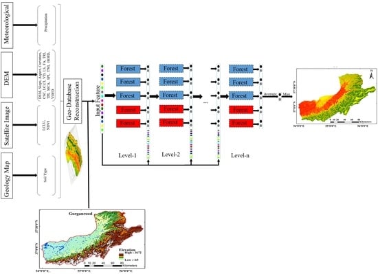
FSM can be applied in three main steps: (1) preprocessing and data preparation, (2) model training and tuning models’ parameters, and (3) applying the trained model to generate FSM and accuracy assessment. The general framework of the proposed FSM method is shown in Figure 1. More details of each step are provided in the following subsections.
2.1. Study Areas
The proposed FSM model was applied to two study areas in Iran. These study areas were the Gorganrud and Karun basins (Figure 2).
The Karun basin originates from the west slopes of the Zagros mountain in Iran, and flows through the plain of Khuzestan. Karun River’s watershed is part of the first-class watershed of the Persian Gulf and the Sea of Oman. The Karun basin has an area of 67,297 km2, which makes it the largest watershed in Iran. The basin lies within the middle Zagros highlands and is bounded by 30°00′ to 34°05′N latitudes and 48°00′ to 52°30′E longitudes.
The Gorganrud Basin, located in the province of Golestan, is one of the most flood-prone watersheds in Northern Iran. It occupies an area of 11,290 km2 located between 36°25′ to 38°15′N latitudes and 56°26′ to 54°10′E longitudes. There is a semi-arid, semi-humid, humid, and Mediterranean climate in this basin with a mean annual temperature of about 18 °C. Over the last decade, there have been multiple large flood events in this basin; the largest one occurred on 11 August 2001, which killed more than 500 people. Furthermore, on 17 March 2019, over 70 villages, 12,000 homes, infrastructure, gardens, and agricultural lands were destroyed by a flood.
2.2. Flood Samples
Flood maps are essential for generating samples of flooded and non-flooded points. In this study, the reports published by the Iranian Water Resources Department for the period of 1985–2022 as well as investigative reports on disaster management for the flood events in the two study areas were used to create the samples. A field survey was also conducted to verify the data collected regarding flooded locations. Based on the flood susceptibility maps obtained by the Multi-Criteria Decision Making (MCDM) analysis, areas with lower flood susceptibility ranks were recognized. Non-flooded points were randomly created in those areas in the GIS software. Finally, the samples of flooded and non-flooded areas were divided into two groups of training, and test datasets (Table 1).
2.3. Flood Conditioning Factors
Current research considers 21 independent factors which affect FSM, shown in Table 2. The flood conditioning factors for both study areas are also illustrated in Figure 3 and Figure 4. These factors were derived from Sentinel-1 and Sentinel-2, Landsat satellite imagery, DEM, and in-situ precipitation data. A total of 17 factors from the 21 investigated flood conditioning factors were calculated using DEM and 3D topography indicators.
2.4. Cascade Forest Model (CFM)
DNNs have a large number of hidden neurons, which learn representations layer-by-layer by leveraging forward and backward propagation procedures [50]. In contrast, CFM creates a cascade of Decision Tree (DT) forests to learn classification distributions (features) based on layers of input data, supervised by the input data [48]. Therefore, CFM generates more accurate predictions based on ensembles of random forests because each layer learns more discriminative representations [51,52].
As illustrated in Figure 5, a CFM consists of multiple layers, each of which consists of an ensemble module. Each layer receives features by concatenation of the input and output probabilistic features from the previous layer, then feeds the results to the next level [47]. For each layer, the process is repeated, and the final output is produced by averaging the forest outputs (without raw data) using the argmax function. To ensure that the ensemble is diverse, each layer includes different types of forests (the red and blue boxes in Figure 5).
The concatenation probabilistic features with original input features put into a single input feature vector can effectively prevent overfitting. The output of CFM, , for original input vector dataset, , for layer can be described as:
where refers to individual learner (i.e., RF algorithm) and n is number of individual learners.
2.5. Feature Selection
The feature selection process is important for dimensional reduction of the input datasets. This process removes the less effective features from the input dataset. The main purpose of using feature selection is to improve learning accuracy and to minimize the computational costs and time during the model training [53].
Heuristic strategies are utilized to determine a reasonably informative feature subset from the entire solution space, which may not be the best solution but will be accepted within the constraints of computational efficiency [54]. In Ref. [55], HHO was proposed as a population-based, nature-inspired optimization paradigm to select the optimum features. This optimization algorithm has widely been used in many applications of remote sensing [56]. HHO was inspired by the Harris’ hawks in nature and their cooperative behaviors, in which several hawks attack their prey from different directions to surprise them. Based on dynamic scenarios and prey escaping patterns, Harris’ hawks can present a variety of chasing patterns [57].
In terms of optimization, HHO is a continuous algorithm. Some real-world problems, such as feature selection, have a binary search space. Consequently, this algorithm should be reformulated efficiently to work on binary spaces. Thus, this study used the binary version of the HHO algorithm for feature selection.
2.6. Accuracy Assessment
The accuracy assessment was carried out by both visual interpretation of the results and statistical accuracy measures, such as Overall Accuracy (OA), Balance Accuracy (BA), F1-Score, Kappa Coefficient (KC), Area Under the Receiver Operating Characteristic (ROC) Curve (AUC), and Intersection Over Union (IOU). The OA index shows the overall performance of the model. The misbalancing of sample datasets is one the most important challenges in FSM using machine learning models. Therefore, different indices, such as such as BA, KC, and F1-score, were calculated to have a better evaluation of the model in an imbalanced dataset.
Moreover, to assess the effectiveness of the CFM, its performance was also compared to other advanced and well-known machine learning approaches, including SVM, DT, RF, LightGBM, DNN, XGboost, and CatBoost.
3. Results
All implemented models in this study have several hyperparameters that need to be tuned. These hyperparameters were knowledge-based, and the optimal values were selected based on trial and error (Table 3).
3.1. Variable Dependency
This study used 21 flood conditioning factors for FSM. Figure 6 shows the correlation between variables based on the Pearson correlation Coefficient (PCC) for the Karun and Gorganrud basins. Based on the results, the correlation between the independent variables was low (under 0.5). However, the correlation between the dependent variables (e.g., TRI and Slope factors) was more than 0.7.
A variance inflation factor (VIF) was employed to calculate the degree of multicollinearity among multiple predictor factors. The result of the VIF for the Karun and Gorganrud basins is shown in Figure 7. VIF values equal to 1, between 1 up to 5, and more than 5 indicate no correlation, moderate correlation, and high correlation between variables, respectively.
3.2. FSM of the Karun Basin
Figure 8 illustrates the results of FSM by different models for the Karun basin. Most areas are located in the low to very low susceptibility regions. The high flood susceptibility areas are in the southwest part of the Karun basin. Furthermore, some small high flood-prone regions can be seen in the north of the study area.
Table 4 presents the statistical indices used to compare the accuracy of different models. The ensemble learning models (i.e., RF and DT) provided higher performance, while other non-ensemble models, such as DNN and SVM had relatively lower accuracy. Among ensemble learning methods, the proposed CFM achieved the highest performance considering all accuracy indices. CFM resulted in an OA of more than 94.04, which was higher than SVM, RF, DNN, DT, LightGBM, CatBoost, and XGBoost by 8.70%, 1.06%, 6.32%, 3.79%, 0.40%, 0.46%, and 0.46%, respectively. Furthermore, the proposed CFM improved the results of the F1-Score index, which was approximately 12–0.76% compared to all other models.
A comparison of confusion matrices for different FSM models in the Karun basin is demonstrated in Figure 9. The CatBoost model correctly classified 1960 and 882 non-flooded and flooded samples, which had the highest performance in detecting non-flooded areas. However, its performance for the flooded class was quite low. The LightGBM model correctly classified nine samples more than the proposed CFM model regarding the non-flooded class; however, it missed 21 samples in the flooded class. Additionally, although the XGBoost model also provided a performance equal to the CFM algorithm in the non-flooded class, it missed 14 samples in the flooded class. Overall, the proposed CFM had the best performance in both flooded and non-flooded classes. CFM correctly classified 1950 (906) samples of the non-flooded (flooded) samples.
Figure 10 illustrates the ROC curves of FSM models. The results indicated that the CFM achieved the highest AUC value (0.97). The CatBoost and XgBoost models were second best models with AUC = 0.96, the LightGBM model was third with AUC = 0.96. The AUC of other models was lower than 0.96.
3.3. FSM of the Gorganrud Basin
The results of FSM models for the Gorganrud basin are shown in Figure 11. Overall, the west side of the Gorganrud basin is located in the high flood-prone zones. However, the east side of the basin is classified as a low flood susceptibility region.
The accuracy assessment of the FSM models in the Gorganrud basin is shown in Table 5. The proposed CFM had the best performance considering all indices. For instance, the OA of the CFM is 92.40 %, which is 3.13%, 0.89%, and 2.01% higher than the XGBoost, CatBoost, and LightGBM models, respectively. Additionally, CFM has a significant improvement compared to other remaining models. For example, it outperformed the SVM, RF, DNN, and DT methods by more than 1.57%, 3.46%, 5.7%, and 4.8% in terms of the OA index, respectively.
The confusion matrices of different FSM models over the Gorganrud basin are shown in Figure 12. Most models showed better performance in detecting the non-flooded areas compared to the flood regions. For example, among 419 flooded samples, the LightGBM and CFM correctly classified 372 and 371 samples, respectively. Although the CatBoost model had slightly better accuracy in identifying the flooded class compared to the proposed LightGBM, it had lower accuracy in detecting non-flooded samples. Overall, CFM had the best performance compared to other SFM models.
The FSM results over the Gorganrud basin were evaluated using the ROC curve for all models (Figure 13). Overall, the and models were the most efficient ones. The DT model provided the lowest performance among FSM models with AUC = 0.876. The remaining five FSM models (SVM, RF, DNN, XGBoost, and LightGBM) also had a lower AUC compared to CFM.
4. Discussion
4.1. Accuracy of the Proposed CFM
This study has introduced an advanced machine-learning model for FSM. The accuracy of the proposed CFM was compared with those of seven other FSM models over two different study areas. The results showed that CFM had better performance, with an OA of 92%. Furthermore, CFM showed higher accuracy in identifying both flood and non-flood classes. Thus, the proposed model could be more robust when unbalanced samples are employed for FSM. One reason for the accuracy improvement was the fact that the proposed model was developed based on a set of random forests in different layers. Another reason was the fact that this model could adapt itself to all the included features. Since the current study utilized a high number of features, the accuracy of the model increased compared to other models.
Recently, many studies have focused on machine learning-based FSM. For instance, Arabameri et al. [58] evaluated the performance of XGBoost, SVM, RF, and Logistic regression for FSM. Their results showed that XGBoost provided more promising results than other models. Furthermore, Kaiser, et al. [59] estimated the performance of Gradient Boosting Decision Tree, RF, and Catboost models. Their results showed that Catboost had more reliable results. Similarly, in the current study, the result of FSM implemented for two study areas showed that Catboost and XGBoost models outperformed other algorithms.
It is worth noting that there is a tradeoff between flooded and non-flooded classification using machine learning models. Based on the presented confusion matrices in Figure 9 and Figure 12, some differences for the flooded and non-flooded classes were observed. For instance, a comparison between Figure 12e,h showed that the performance of the LightGBM and CFM models was not similar. Thus, the proposed method had a high level of effectiveness in both flooded and non-flooded classes.
The complexity of the study area could negatively affect the results of FSM produced by machine learning models. For example, most models had lower accuracies in the Gorganrud basin compared to the Karun basin. However, the results of CFM over both study areas were high. Thus, the proposed CFM could show robust and better results in various study areas with different characteristics.
4.2. Flood Susceptible Areas
A generated flood susceptibility map can help decision makers in identifying flood prone areas. In Figure 14, some of flood susceptible areas in Karun basin are shown. As is noticeable, flood inventory points are overlaid with areas, which have a high flood susceptibility index. In Karun basin, prone areas are mostly located in the west-southern part, due to the fact that the values of important factors in this area are in line with higher flood susceptibility. For instance, the value of elevation (DEM), distance to stream (HOFD), slope is low, and the level of wetness index (TWI) and catchment area (MCA) is high. The same condition is true for other regions demonstrated in the figure such as northern and eastern parts.
Figure 15 is the zoom area of highly susceptible areas in the Gorganrud basin. As it can be seen in this figure, flooded points are located in regions where the susceptibility index is high. In this basin, the western zone as well as some parts of the central and eastern zones which are illustrated in the figure are recognized as flood prone areas.
4.3. Feature Selection
This study applied the HHO-based optimization framework for feature selection. In this regard, the HHO algorithm and CFM were used together for feature selection using the Karun sample dataset. The result of the feature selection process indicated that the highest accuracy can be obtained by using 12 optimal features. After removing three features including Cross Sectional Curvature, Curve Number (CN), and Land Use/Land Cover (LULC) from the input dataset, the value of OA (93.84%) remained unchanged. The elimination of these features had only 0.2% impact on the OA. Therefore, it can be concluded that these features do not have a key role in achieving promising results.
4.4. Model Generalization
The training samples dataset are important for machine learning-based FSM models, which might not be available in all areas. Thus, utilizing a pre-trained model can be a reasonable solution for such conditions. In this study, we evaluated the generalization of the proposed CFM by employing a trained model in two scenarios: (1) training the model using the training samples of the Karun basin and evaluating the accuracy of the CFM using the test samples of the Gorganrud basin, and (2) training the model using the training samples of the Gorganrud basin and evaluating the accuracy of the CFM using the test samples of the Karun basin.
The qualitative results of the generalization of different models for the first and second scenarios are provided in Table 6 and Table 7, respectively. Overall, the performance of most models including the proposed CFM, was better in the second scenario than that of the first scenario. As seen, it has provided an acceptable result in the FSM, with an accuracy of more than 79% by the OA index.
It is worth noting that both study areas have similar topographic, geomorphologic and LULC conditions. Moreover, most of the investigated factors which are related to the topography and geomorphology have a similar range of values in the different areas (Table 2). Therefore, the proposed method has provided efficient and robust FSM results.
4.5. Dimension Reduction Impact on FSM
Feature selection is a kind of dimension reduction technique which selects the informative features based on different approaches. The filter-based feature selection approach investigates the features based on a similarity measurement metric such as Pearson Correlation Coefficient (PCC). The mentioned approach was used in order to detect highly correlated features according to a threshold equal to 0.7. Consequently, some features, namely, TRI, SPI, Curvature, VOFD, VD and LSF were eliminated from the dataset. Table 8 illustrates the performance of different models over the Karun basin before dimension reduction process.
After implementing the dimension reduction analysis and eliminating the correlated features, the result of all the models saw an increase in accuracy. By comparing Table 4 and Table 8, it is concluded that SVM method experienced a noticeable accuracy improvement due to the reason that in the SVM algorithm, features’ dependency affects the performance of the model. Moreover, tree-based algorithms consider the features as independent variables. Therefore, dimension reduction does not greatly increase the efficiency of this kind of approaches. However, it leads to a reduction in computational cost in all the applied approaches by decreasing the number of features from 21 to 15.
5. Conclusions
FSM is one of the most important steps to prevent damage from flood events. In this study, the effectiveness of a new advanced machine learning method, CFM, was investigated for FSM. We employed two large-scale datasets for evaluating the performance of the CFM. Additionally, 21 flood conditioning factors were generated to obtain high accuracy. In the Karun basin, prone areas were mostly located in the west-southern part. The flood prone areas of the Gorganrud basin were also located in the western zone as well as some part of the central and eastern zones. For both study areas, the flood inventory points are overlaid with areas with high flood susceptibility values. The accuracy of CFM was compared with those of seven conventional and advanced machine learning models. The proposed CFM outperformed other models in both study areas. CFM provided an OA of more than 92%. Furthermore, the generalization assessment of the models showed that the CFM had a higher generalization capability compared to other models. In this study, we set the model hyperparameters based on several trial and error efforts. Future studies should use automatic methods, such as Genetic algorithm (GA), HHO, particle swarm optimization (PSO) for tuning the hyperparameters of the models.
Author Contributions
Conceptualization, S.T.S. and M.A.; Methodology, S.T.S.; Software, S.T.S. and Y.K.-S.; Validation, S.T.S. and Y.K.-S.; Formal analysis, S.T.S.; Investigation, S.T.S.; Resources, S.T.S. and M.A.; Data curation, S.T.S., Y.K.-S. and R.S.; Writing—original draft, S.T.S.; Writing—review & editing, S.T.S., Y.K.-S., M.H., R.S., J.C. and M.A.; Visualization, S.T.S. and Y.K.-S.; Supervision, M.H. and J.C.; Funding acquisition, M.A. All authors have read and agreed to the published version of the manuscript.
Funding
This work was partially supported by the AXA Research Fund.
Data Availability Statement
Publicly available datasets were analyzed in this study.
Acknowledgments
We thank the anonymous reviewers for their valuable comments on our manuscript. This research was partially supported by the AXA fund for research.
Conflicts of Interest
The authors declare no conflict of interest.
References
- Seydi, S.T.; Hasanlou, M.; Chanussot, J. Burnt-Net: Wildfire burned area mapping with single post-fire Sentinel-2 data and deep learning morphological neural network. Ecol. Indic. 2022, 140, 108999. [Google Scholar] [CrossRef]
- Shimada, G. The impact of climate-change-related disasters on africa’s economic growth, agriculture, and conflicts: Can humanitarian aid and food assistance offset the damage? Int. J. Environ. Res. Public Health 2022, 19, 467. [Google Scholar] [CrossRef] [PubMed]
- Zhang, Z.; Luo, C.; Zhao, Z. Application of probabilistic method in maximum tsunami height prediction considering stochastic seabed topography. Nat. Hazards 2020, 104, 2511–2530. [Google Scholar] [CrossRef]
- Mahdavi, S.; Salehi, B.; Huang, W.; Amani, M.; Brisco, B. A PolSAR change detection index based on neighborhood information for flood mapping. Remote Sens. 2019, 11, 1854. [Google Scholar] [CrossRef] [Green Version]
- Glago, F.J. Flood disaster hazards; causes, impacts and management: A state-of-the-art review. In Natural Hazards-Impacts, Adjustments and Resilience; IntechOpen: London, UK, 2021. [Google Scholar] [CrossRef]
- Seydi, S.T.; Saeidi, V.; Kalantar, B.; Ueda, N.; van Genderen, J.; Maskouni, F.H.; Aria, F.A. Fusion of the Multisource Datasets for Flood Extent Mapping Based on Ensemble Convolutional Neural Network (CNN) Model. J. Sens. 2022, 2022, 2887502. [Google Scholar] [CrossRef]
- Kinouchi, T.; Sayama, T. A comprehensive assessment of water storage dynamics and hydroclimatic extremes in the Chao Phraya River Basin during 2002–2020. J. Hydrol. 2021, 603, 126868. [Google Scholar]
- Sharifipour, M.; Amani, M.; Moghimi, A. Flood Damage Assessment Using Satellite Observations within the Google Earth Engine Cloud Platform. J. Ocean Technol. 2022, 17, 65–75. [Google Scholar]
- Parsian, S.; Amani, M.; Moghimi, A.; Ghorbanian, A.; Mahdavi, S. Flood hazard mapping using fuzzy logic, analytical hierarchy process, and multi-source geospatial datasets. Remote Sens. 2021, 13, 4761. [Google Scholar] [CrossRef]
- Duan, Y.; Xiong, J.; Cheng, W.; Wang, N.; He, W.; He, Y.; Liu, J.; Yang, G.; Wang, J.; Yang, J. Assessment and spatiotemporal analysis of global flood vulnerability in 2005–2020. Int. J. Disaster Risk Reduct. 2022, 80, 103201. [Google Scholar] [CrossRef]
- Pollack, A.B.; Sue Wing, I.; Nolte, C. Aggregation bias and its drivers in large-scale flood loss estimation: A Massachusetts case study. J. Flood Risk Manag. 2022, 15, e12851. [Google Scholar] [CrossRef]
- Abd Rahman, N.; Tarmudi, Z.; Rossdy, M.; Muhiddin, F.A. Flood mitigation measres using intuitionistic fuzzy dematel method. Malays. J. Geosci. 2017, 1, 1–5. [Google Scholar] [CrossRef]
- Gazi, M.Y.; Islam, M.A.; Hossain, S. flood-hazard mapping in a regional scale way forward to the future hazard atlas in Bangladesh. Malays. J. Geosci. 2019, 3, 1–11. [Google Scholar] [CrossRef]
- Khojeh, S.; Ataie-Ashtiani, B.; Hosseini, S.M. Effect of DEM resolution in flood modeling: A case study of Gorganrood River, Northeastern Iran. Nat. Hazards 2022, 112, 2673–2693. [Google Scholar] [CrossRef]
- Parizi, E.; Khojeh, S.; Hosseini, S.M.; Moghadam, Y.J. Application of Unmanned Aerial Vehicle DEM in flood modeling and comparison with global DEMs: Case study of Atrak River Basin, Iran. J. Environ. Manag. 2022, 317, 115492. [Google Scholar] [CrossRef]
- Balogun, A.-L.; Sheng, T.Y.; Sallehuddin, M.H.; Aina, Y.A.; Dano, U.L.; Pradhan, B.; Yekeen, S.; Tella, A. Assessment of data mining, multi-criteria decision making and fuzzy-computing techniques for spatial flood susceptibility mapping: A comparative study. Geocarto Int. 2022, 1–27. [Google Scholar] [CrossRef]
- Youssef, A.M.; Pradhan, B.; Dikshit, A.; Mahdi, A.M. Comparative study of convolutional neural network (CNN) and support vector machine (SVM) for flood susceptibility mapping: A case study at Ras Gharib, Red Sea, Egypt. Geocarto Int. 2022, 1–28. [Google Scholar] [CrossRef]
- Ha, H.; Bui, Q.D.; Nguyen, H.D.; Pham, B.T.; Lai, T.D.; Luu, C. A practical approach to flood hazard, vulnerability, and risk assessing and mapping for Quang Binh province, Vietnam. Environ. Dev. Sustain. 2022, 1–30. [Google Scholar] [CrossRef]
- Mudashiru, R.B.; Sabtu, N.; Abustan, I. Quantitative and semi-quantitative methods in flood hazard/susceptibility mapping: A review. Arab. J. Geosci. 2021, 14, 1–24. [Google Scholar]
- Vojinović, Z.; Golub, D.; Weesakul, S.; Keerakamolchai, W.; Hirunsalee, S.; Meesuk, V.; Sanchez-Torres, A.; Kumara, S. Merging Quantitative and Qualitative Analyses for Flood Risk Assessment at Heritage Sites, The Case of Ayutthaya, Thailand. In Proceedings of the 11th International Conference on Hydroinformatics, New York, NY, USA, 17–21 August 2014. [Google Scholar]
- Kanani-Sadat, Y.; Arabsheibani, R.; Karimipour, F.; Nasseri, M. A new approach to flood susceptibility assessment in data-scarce and ungauged regions based on GIS-based hybrid multi criteria decision-making method. J. Hydrol. 2019, 572, 17–31. [Google Scholar] [CrossRef]
- Pathan, A.I.; Girish Agnihotri, P.; Said, S.; Patel, D. AHP and TOPSIS based flood risk assessment-a case study of the Navsari City, Gujarat, India. Environ. Monit. Assess. 2022, 194, 1–37. [Google Scholar]
- Dano, U.L. An AHP-based assessment of flood triggering factors to enhance resiliency in Dammam, Saudi Arabia. GeoJournal 2022, 87, 1945–1960. [Google Scholar] [CrossRef]
- Chang, L.-C.; Liou, J.-Y.; Chang, F.-J. Spatial-temporal flood inundation nowcasts by fusing machine learning methods and principal component analysis. J. Hydrol. 2022, 612, 128086. [Google Scholar] [CrossRef]
- Ahmad, M.; Al Mehedi, M.A.; Yazdan, M.M.S.; Kumar, R. Development of Machine Learning Flood Model Using Artificial Neural Network (ANN) at Var River. Liquids 2022, 2, 147–160. [Google Scholar] [CrossRef]
- Chen, H.; Yang, D.; Hong, Y.; Gourley, J.J.; Zhang, Y. Hydrological data assimilation with the Ensemble Square-Root-Filter: Use of streamflow observations to update model states for real-time flash flood forecasting. Adv. Water Resour. 2013, 59, 209–220. [Google Scholar] [CrossRef]
- Anjum, M.N.; Ding, Y.; Shangguan, D.; Tahir, A.A.; Iqbal, M.; Adnan, M. Comparison of two successive versions 6 and 7 of TMPA satellite precipitation products with rain gauge data over Swat Watershed, Hindukush Mountains, Pakistan. Atmos. Sci. Lett. 2016, 17, 270–279. [Google Scholar] [CrossRef] [Green Version]
- Batelaan, O.; De Smedt, F. WetSpass: A flexible, GIS based, distributed recharge methodology for regional groundwater. In Impact of Human Activity on Groundwater Dynamics, Proceedings of the International Symposium (Symposium S3) Held During the Sixth Scientific Assembly of the International Association of Hydrological Sciences (IAHS), Maastricht, The Netherlands, 18–27 July 2001; International Association of Hydrological Sciences: Wallingford, UK, 2001; p. 11. [Google Scholar]
- Liu, Z.; Martina, M.L.; Todini, E. Flood forecasting using a fully distributed model: Application of the TOPKAPI model to the Upper Xixian Catchment. Hydrol. Earth Syst. Sci. 2005, 9, 347–364. [Google Scholar] [CrossRef] [Green Version]
- Liu, J.; Xiong, J.; Cheng, W.; Li, Y.; Cao, Y.; He, Y.; Duan, Y.; He, W.; Yang, G. Assessment of flood susceptibility using support vector machine in the belt and road region. Nat. Hazards Earth Syst. Sci. Discuss. 2021, 1–37. [Google Scholar] [CrossRef]
- Mousavi, S.M.; Ataie-Ashtiani, B.; Hosseini, S.M. Comparison of statistical and mcdm approaches for flood susceptibility mapping in northern iran. J. Hydrol. 2022, 612, 128072. [Google Scholar] [CrossRef]
- Tung, Y.-K. River flood routing by nonlinear Muskingum method. J. Hydraul. Eng. 1985, 111, 1447–1460. [Google Scholar] [CrossRef] [Green Version]
- Prasad, P.; Loveson, V.J.; Das, B.; Kotha, M. Novel ensemble machine learning models in flood susceptibility mapping. Geocarto Int. 2022, 37, 4571–4593. [Google Scholar] [CrossRef]
- Avand, M.; Kuriqi, A.; Khazaei, M.; Ghorbanzadeh, O. DEM resolution effects on machine learning performance for flood probability mapping. J. Hydro-Environ. Res. 2022, 40, 1–16. [Google Scholar] [CrossRef]
- Saber, M.; Boulmaiz, T.; Guermoui, M.; Abdrabo, K.I.; Kantoush, S.A.; Sumi, T.; Boutaghane, H.; Nohara, D.; Mabrouk, E. Examining LightGBM and CatBoost models for wadi flash flood susceptibility prediction. Geocarto Int. 2021, 1–26. [Google Scholar] [CrossRef]
- Ma, M.; Zhao, G.; He, B.; Li, Q.; Dong, H.; Wang, S.; Wang, Z. XGBoost-based method for flash flood risk assessment. J. Hydrol. 2021, 598, 126382. [Google Scholar] [CrossRef]
- Ha, M.C.; Vu, P.L.; Nguyen, H.D.; Hoang, T.P.; Dang, D.D.; Dinh, T.B.H.; Şerban, G.; Rus, I.; Brețcan, P. Machine Learning and Remote Sensing Application for Extreme Climate Evaluation: Example of Flood Susceptibility in the Hue Province, Central Vietnam Region. Water 2022, 14, 1617. [Google Scholar] [CrossRef]
- Yaseen, A.; Lu, J.; Chen, X. Flood susceptibility mapping in an arid region of Pakistan through ensemble machine learning model. Stoch. Environ. Res. Risk Assess. 2022, 36, 3041–3061. [Google Scholar] [CrossRef]
- Costache, R.; Țîncu, R.; Elkhrachy, I.; Pham, Q.B.; Popa, M.C.; Diaconu, D.C.; Avand, M.; Costache, I.; Arabameri, A.; Bui, D.T. New neural fuzzy-based machine learning ensemble for enhancing the prediction accuracy of flood susceptibility mapping. Hydrol. Sci. J. 2020, 65, 2816–2837. [Google Scholar] [CrossRef]
- Seydi, S.T.; Hasanlou, M.; Chanussot, J. DSMNN-Net: A Deep Siamese Morphological Neural Network Model for Burned Area Mapping Using Multispectral Sentinel-2 and Hyperspectral PRISMA Images. Remote Sens. 2021, 13, 5138. [Google Scholar] [CrossRef]
- Seydi, S.T.; Shah-Hosseini, R.; Amani, M. A Multi-Dimensional Deep Siamese Network for Land Cover Change Detection in Bi-Temporal Hyperspectral Imagery. Sustainability 2022, 14, 12597. [Google Scholar] [CrossRef]
- Liao, L.; Du, L.; Guo, Y. Semi-supervised SAR target detection based on an improved faster R-CNN. Remote Sens. 2021, 14, 143. [Google Scholar] [CrossRef]
- Seydi, S.T.; Hasanlou, M.; Amani, M.; Huang, W. Oil spill detection based on multiscale multidimensional residual CNN for optical remote sensing imagery. IEEE J. Sel. Top. Appl. Earth Obs. Remote Sens. 2021, 14, 10941–10952. [Google Scholar] [CrossRef]
- Seydi, S.T.; Hasanlou, M.; Chanussot, J. A Quadratic Morphological Deep Neural Network Fusing Radar and Optical Data for the Mapping of Burned Areas. IEEE J. Sel. Top. Appl. Earth Obs. Remote Sens. 2022, 15, 4194–4216. [Google Scholar] [CrossRef]
- Zhao, L.; Wang, L. A new lightweight network based on MobileNetV3. KSII Trans. Internet Inf. Syst. (TIIS) 2022, 16, 1–15. [Google Scholar]
- Chen, J.; Du, L.; Guo, Y. Label constrained convolutional factor analysis for classification with limited training samples. Inf. Sci. 2021, 544, 372–394. [Google Scholar] [CrossRef]
- Zhou, Z.-H.; Feng, J. Deep forest. Natl. Sci. Rev. 2019, 6, 74–86. [Google Scholar] [CrossRef]
- Zhou, Z.-H.; Feng, J. Deep Forest: Towards An Alternative to Deep Neural Networks. In Proceedings of the IJCAI, Melbourne, Australia, 19–25 August 2017; pp. 3553–3559. [Google Scholar]
- Jamali, A.; Mahdianpari, M.; Brisco, B.; Granger, J.; Mohammadimanesh, F.; Salehi, B. Deep Forest classifier for wetland mapping using the combination of Sentinel-1 and Sentinel-2 data. GIScience Remote Sens. 2021, 58, 1072–1089. [Google Scholar] [CrossRef]
- Yang, F.; Xu, Q.; Li, B.; Ji, Y. Ship detection from thermal remote sensing imagery through region-based deep forest. IEEE Geosci. Remote Sens. Lett. 2018, 15, 449–453. [Google Scholar] [CrossRef]
- Cheng, J.; Chen, M.; Li, C.; Liu, Y.; Song, R.; Liu, A.; Chen, X. Emotion recognition from multi-channel eeg via deep forest. IEEE J. Biomed. Health Inform. 2020, 25, 453–464. [Google Scholar] [CrossRef]
- Zhang, L.; Sun, H.; Rao, Z.; Ji, H. Hyperspectral imaging technology combined with deep forest model to identify frost-damaged rice seeds. Spectrochim. Acta Part A Mol. Biomol. Spectrosc. 2020, 229, 117973. [Google Scholar] [CrossRef] [PubMed]
- Mahdavi, S.; Salehi, B.; Amani, M.; Granger, J.; Brisco, B.; Huang, W. A dynamic classification scheme for mapping spectrally similar classes: Application to wetland classification. Int. J. Appl. Earth Obs. Geoinf. 2019, 83, 101914. [Google Scholar] [CrossRef]
- Taradeh, M.; Mafarja, M.; Heidari, A.A.; Faris, H.; Aljarah, I.; Mirjalili, S.; Fujita, H. An evolutionary gravitational search-based feature selection. Inf. Sci. 2019, 497, 219–239. [Google Scholar] [CrossRef]
- Heidari, A.A.; Mirjalili, S.; Faris, H.; Aljarah, I.; Mafarja, M.; Chen, H. Harris hawks optimization: Algorithm and applications. Future Gener. Comput. Syst. 2019, 97, 849–872. [Google Scholar] [CrossRef]
- Seydi, S.T.; Akhoondzadeh, M.; Amani, M.; Mahdavi, S. Wildfire damage assessment over Australia using sentinel-2 imagery and MODIS land cover product within the google earth engine cloud platform. Remote Sens. 2021, 13, 220. [Google Scholar] [CrossRef]
- Islam, M.Z.; Wahab, N.I.A.; Veerasamy, V.; Hizam, H.; Mailah, N.F.; Guerrero, J.M.; Mohd Nasir, M.N. A Harris Hawks optimization based single-and multi-objective optimal power flow considering environmental emission. Sustainability 2020, 12, 5248. [Google Scholar] [CrossRef]
- Arabameri, A.; Chandra Pal, S.; Costache, R.; Saha, A.; Rezaie, F.; Seyed Danesh, A.; Pradhan, B.; Lee, S.; Hoang, N.-D. Prediction of gully erosion susceptibility mapping using novel ensemble machine learning algorithms. Geomat. Nat. Hazards Risk 2021, 12, 469–498. [Google Scholar] [CrossRef]
- Kaiser, M.; Günnemann, S.; Disse, M. Regional-scale prediction of pluvial and flash flood susceptible areas using tree-based classifiers. J. Hydrol. 2022, 612, 128088. [Google Scholar] [CrossRef]
Figure 1.
Overview of the proposed Flood Susceptibility Mapping (FSM) based on the Cascade Forest Model (CFM). Digital Elevation Model (DEM), Cross-Sectional Curvature (CSC), Longitudinal Curvature (LC), Convergence Index (CI), Valley Depth (VD), LS factor (LS), Flow Accumulation (FA), Terrain Ruggedness Index (TRI), Topographic Position Index (TPI), Modified Catchment Area (MCA), Stream Power Index (SPI), Topographic Wetness Index (TWI), Horizontal Overland Flow Distance (HOFD), Vertical Overland Flow Distance (VOFD), Land Use/Land Cover Map (LULC), and Normalized Vegetation Index (NDVI).

Figure 2.
Location of the study areas and flood inventories.

Figure 3.
The produced flood conditioning factors for FSM in the Karun basin. (a) DEM, (b) Slope, (c) Aspect, (d) Curvature, (e) Cross-Sectional Curvature, (f) Longitudinal Curvature, (g) Convergence Index, (h) Valley Depth, (i) LS factor, (j) Flow Accumulation, (k) Terrain Ruggedness, (l) Topographic Position Index, (m) Modified Catchment Area, (n) Stream Power Index, (o) Topographic Wetness Index, (p) Horizontal Overland Flow Distance, (q) Vertical Overland Flow Distance, (r) Curve Number, (s) Land Use/Land Cover Map, (t) Normalized Vegetation Index, and (u) Modified Fournier Index.


Figure 4.
The produced flood conditioning factors for FSM in the Gruganrud basin. (a) DEM, (b) Slope, (c) Aspect, (d) Curvature, (e) Cross-Sectional Curvature, (f) Longitudinal Curvature, (g) Convergence Index, (h) Valley Depth, (i) LS factor, (j) Flow Accumulation, (k) Terrain Ruggedness, (l) Topographic Position Index, (m) Modified Catchment Area, (n) Stream Power Index, (o) Topographic Wetness Index, (p) Horizontal Overland Flow Distance, (q) Vertical Overland Flow Distance, (r) Curve Number, (s) Land Use/Land Cover Map, (t) Normalized Vegetation Index, and (u) Modified Fournier Index.


Figure 5.
Illustration of the structure of a Cascade Forest Model (CFM).

Figure 6.
Pearson correlation coefficient between all variables. (a) Karun Basin, and (b) Gorganrud Basin.
Figure 6.
Pearson correlation coefficient between all variables. (a) Karun Basin, and (b) Gorganrud Basin.


Figure 7.
Variance Inflation Factor (VIF) of all variables. (a) Karun Basin, and (b) Gorganrud Basin.
Figure 7.
Variance Inflation Factor (VIF) of all variables. (a) Karun Basin, and (b) Gorganrud Basin.


Figure 8.
Comparison of the FSM for the Karun basin: (a) Support Vector Machine (SVM), (b) Random Forest (RF), (c) Deep Neural Network (DNN), (d) Decision Tree (DT), (e) Light Gradient Boosting Machine (LightGBM), (f) Categorical Boosting (CatBoost), (g) Extreme Gradient Boosting (XGBoost), and (h) Cascade Forest Model (CFM).

Figure 9.
Comparing the confusion matrices of different FSM models in the Karun basin. (a) Support Vector Machine (SVM), (b) Random Forest (RF), (c) Deep Neural Network (DNN), (d) Decision Tree (DT), (e) Light Gradient Boosting Machine (LightGBM), (f) Categorical Boosting (CatBoost), (g) Extreme Gradient Boosting (XGBoost), and (h) Cascade Forest Model (CFM).

Figure 10.
A comparison of the ROC curves and AUC values of different FSM models using the test dataset. Support Vector Machine (SVM), Random Forest (RF), Deep Neural Network (DNN), Decision Tree (DT), Light Gradient Boosting Machine (LightGBM), Categorical Boosting (CatBoost), Extreme Gradient Boosting (XGBoost), and Cascade Forest Model (CFM).

Figure 11.
The FSM maps derived from different models for the Gorganrud basin: (a) Support Vector Machine (SVM), (b) Random Forest (RF), (c) Deep Neural Network (DNN), (d) Decision Tree (DT), (e) Light Gradient Boosting Machine (LightGBM), (f) Categorical Boosting (CatBoost), (g) Extreme Gradient Boosting (XGBoost), and (h) Cascade Forest Model (CFM).

Figure 12.
Comparing the confusion matrices of different SFM models in the Gorganrud basin. (a) Support Vector Machine (SVM), (b) Random Forest (RF), (c) Deep Neural Network (DNN), (d) Decision Tree (DT), (e) Light Gradient Boosting Machine (LightGBM), (f) Categorical Boosting (CatBoost), (g) Extreme Gradient Boosting (XGBoost), and (h) Cascade Forest Model (CFM).

Figure 13.
A comparison of the ROC curves and AUC values of the 8 models using the test dataset for Gorganrud basin. Support Vector Machine (SVM), Random Forest (RF), Deep Neural Network (DNN), Decision Tree (DT), Light Gradient Boosting Machine (LightGBM), Categorical Boosting (CatBoost), Extreme Gradient Boosting (XGBoost), and Cascade Forest Model (CFM).

Figure 14.
Examples of highly susceptible areas in the Karun basin.

Figure 15.
Examples of highly susceptible areas in the Gorganrud basin.


Table 1.
The training and test samples of flooded and non-flooded areas.
| Description | Study Area | Number of Samples | Percentage (%) | Non-Flood | Flood |
|---|---|---|---|---|---|
| Training | Karun | 1123 | 27 | 747 | 376 |
| Gorganrud | 383 | 30 | 211 | 172 | |
| Test | Karun | 3037 | 73 | 2029 | 1008 |
| Gorganrud | 895 | 70 | 476 | 419 | |
| Total | Karun | 4160 | 100 | 2776 | 1384 |
| Gorganrud | 1278 | 100 | 687 | 591 |
Table 2.
Flood conditioning factors which were used in this study.
| Factor | Description | Basin | Resolution | Source | |
|---|---|---|---|---|---|
| Gorganrud | Karun | ||||
| Digital Elevation Model (DEM) | Elevation is one of the most significant criteria in identifying flood susceptible areas. Areas with lower elevation values are more likely to experience flood. | Max: 3672 Min: −65 | Max: 4418 Min: −66 | 30 m | SRTM 1 |
| Slope | Slope is a criterion that controls run off and flow velocity in a way that the possibility of flood events is accelerated in flat areas. | Max: 3927 Min: 0 | Max: 833 Min: 0 | 30 m | DEM |
| Aspect | Aspect examines the direction of slope which affects many features, such as water flow direction, receiving precipitation, land cover scheme and sunshine. | Max: 359 Min: −1 | Max: 359 Min: 0 | 30 m | DEM |
| Curvature | Geomorphological characteristics of the surface is determined by this criterion which has three classes, namely, convex, concave and flat. | Max: 397 Min: −494 | Max: 193 Min: −138 | 30 m | DEM |
| Plan Curvature | This morphometric criterion identifies the type of surface runoff, and whether it is convergent or divergent and controls the water movement. | Max: 0.467 Min: −0.424 | Max: 0.13 Min: −0.07 | 30 m | DEM |
| Profile Curvature | The level of runoff, whether it is high or low, is identified using this morphometric factor. | Max: 0.475 Min: −0.455 | Max: 0.09 Min: −0.09 | 30 m | DEM |
| Convergence Index | This morphometric criterion corresponds to the river valleys and interfluvial areas using negative and higher than zero values, respectively. | Max: 99 Min: −99 | Max: 99 Min: −99 | 30 m | DEM |
| Valley Depth | This measure estimates the vertical distance from interpolated ridge level to a river network base level for each pixel. | Max: 2222 Min: 0 | Max: 1543 Min: 0 | 30 m | DEM |
| LS Factor (LS) | This quantity has two components, slope length and slope steepness, and it defines the impact of topography on soil erosion. | Max: 248 Min: 0 | Max: 2281 Min: 0 | 30 m | DEM |
| Flow Accumulation (FA) | For each pixel, this criterion indicates the number of pixels which flow into it. Therefore, there is a direct relationship between this factor and flood occurrence possibility. | Max: 1.15 × 10¹⁰ Min: 900 | Max: 6.19 × 10¹⁰ Min: 0 | 30 m | DEM |
| Terrain Ruggedness Index (TRI) | This criterion calculates the elevation difference among a pixel and its adjacent pixels. Flood susceptible areas have a lower TRI value. | Max: 1815 Min: 0 | Max: 390 Min: 0 | 30 m | DEM |
| Topographic Position Index (TPI) | This criterion identifies valleys, ridges, or flat parts of the landscape. Positive and negative values of TPI indicate valleys and ridges, respectively. | Max: 238 Min: −2072 | Max: 461 Min: −332 | 30 m | DEM |
| Modified Catchment Area (MCA) | Catchment area is the area of the upstream watershed. In order to not consider the flow as a thin layer, the modified catchment area can be used to obtain more realistic results. | Max: 1.32 × 10¹⁰ Min: 0 | Max: 5.95 × 10¹⁰ Min: 909 | 30 m | DEM |
| Stream Power Index (SPI) | This hydrological criterion measures the erosive power of the runoff and discharge degree within the catchment area. A higher value of SPI indicates the higher potential of flood occurrence. | Max: 1.61 × 10⁹ Min: 0 | Max: 1.61 × 10⁹ Min: 0 | 30 m | DEM |
| Topographic Wetness Index (TWI) | This index predicts the regions which have a high potential to witness overland runoff. There is a direct relationship between TWI and flooding. | Max: 16 Min: −2 | Max: 27 Min: 1.6 | 30 m | DEM |
| Horizontal Overland Flow Distance (HOFD) | Instead of Euclidean distance from the river network, the horizontal component of water flow is considered. This criterion computes the actual movement of water flow from each pixel to others. Areas with lower value of HOFD are more prone to flooding. | Max: 15,931 Min: 0 | Max: 3008 Min: 0 | 30 m | DEM and Stream |
| Vertical Overland Flow Distance (VOFD) | VOFD is the vertical height difference between each cell and the river network. Areas with lower value of VOFD are more susceptible to flooding. | Max: 1765 Min: 0 | Max: 2581 Min: 0 | 30 m | DEM and Stream |
| Curve Number | This criterion consists of land use data and soil map, and measures the permeability feature of the surface. The amount of penetration is low in areas with high CN values. | Max: 94 Min: 72 | Max: 94 Min: 68 | 250 m | Soil and LULC |
| Land Use/Land Cover (LULC) | The hydrological processes, such as runoff, permeability and evaporation and sediment transportation, vary based on LULC types. | 8 classes | 8 classes | 10 m | ESA 2 |
| Normalized Difference Vegetation Index (NDVI) | NDVI is used to examine the vegetation coverage of the area. There is a negative correlation between compact vegetation cover and flooding. | Max: 0.56 Min: −0.28 | Max: 0.49 Min: −0.19 | 30 m | Landsat Satellite Images |
| Modified Fournier Index (MFI) | The level of precipitation is determined using this criterion. MFI is calculated using monthly and annual average values of rainfall. | Max: 37 Min: 14 | Max: 119 Min: 12 | 30 m | Precipitation |
1 https://www.usgs.gov/ (accessed on 7 November 2022); 2 https://esa-worldcover.org/en (accessed on 7 November 2022).
Table 3.
The optimum values of the tuning parameters of different models. Support Vector Machine (SVM), Random Forest (RF), Deep Neural Network (DNN), Decision Tree (DT), Light Gradient Boosting Machine (LightGBM), Categorical boosting (CatBoost), Extreme Gradient Boosting (XGBoost), and Cascade Forest Model (CFM).
| Method | Optimum Value |
|---|---|
| SVM | Radial Basis Function (RBF) kernel function parameter 10−3, and penalty coefficient 102 |
| RF | Number of trees 155, and the number of randomly selected predictor variables 5 |
| DNN | Number of layers = 5, activation function = rectified linear unit (Relu), number of hidden layers = [150,150,150], weight-initializer = He-Normal, optimizer = ADAM, dropout rate = 0.18 |
| LightGBM | Number of estimators = 150, learning rate = 0.1, regularization parameter = 0.9, number of leaves = 150, and maximum depth = 9 |
| CatBoost | Number of estimators = 105, learning rate = 0.1, and subsample ratio = 0.9 |
| XGBoost | Number of estimators = 105, learning rate = 0.1, maximum depth = 20, and subsample ratio = 0.7 |
| CFM | Number of bins = 90, the maximum number of layers = 8, number of estimator = 5, number of trees = 170, maximum depth = 8, and predictor = XGboost. |
Table 4.
Evaluation of the performance of different FSM models over the Karun basin. OA: overall accuracy; IOU: intersection over union, BA: balance accuracy; KC: kappa coefficient. Support Vector Machine (SVM), Random Forest (RF), Deep Neural Network (DNN), Decision Tree (DT), Light Gradient Boosting Machine (LightGBM), Categorical Boosting (CatBoost), Extreme Gradient Boosting (XGBoost), and Cascade Forest Model (CFM).The highest value is in bold.
| Method | OA (%) | F1-Score (%) | BA (%) | IOU | KC |
|---|---|---|---|---|---|
| SVM | 85.34 | 78.47 | 84.11 | 0.646 | 0.673 |
| RF | 92.98 | 89.29 | 91.75 | 0.806 | 0.840 |
| DNN | 87.72 | 80.10 | 84.39 | 0.668 | 0.713 |
| Decision Tree | 90.25 | 85.17 | 88.76 | 0.741 | 0.779 |
| LightGBM | 93.64 | 90.16 | 92.17 | 82.09 | 0.855 |
| CatBoost | 93.58 | 90.00 | 92.05 | 0.819 | 0.853 |
| XGBoost | 93.58 | 90.14 | 92.29 | 0.820 | 0.854 |
| CFM | 94.04 | 90.92 | 92.99 | 0.833 | 0.865 |
Table 5.
Evaluation of the performance of different FSM models over the Goranrud basin. Support Vector Machine (SVM), Random Forest (RF), Deep Neural Network (DNN), Decision Tree (DT), Light Gradient Boosting Machine (LightGBM), Categorical Boosting (CatBoost), Extreme Gradient Boosting (XGBoost), and Cascade Forest Model (CFM). OA: overall accuracy; IOU: intersection over union, BA: balance accuracy; KC: kappa coefficient. The highest value is in bold.
| Method | OA (%) | F1-Score (%) | BA (%) | IOU | KC |
|---|---|---|---|---|---|
| SVM | 90.83 | 89.54 | 90.41 | 0.811 | 0.815 |
| RF | 88.94 | 87.82 | 88.71 | 0.783 | 0.777 |
| DNN | 86.70 | 83.98 | 85.97 | 0.724 | 0.729 |
| Decision Tree | 87.60 | 86.64 | 87.50 | 0.764 | 0.751 |
| LightGBM | 90.39 | 89.64 | 90.29 | 0.812 | 0.807 |
| CatBoost | 91.51 | 90.57 | 91.24 | 0.828 | 0.829 |
| XGBoost | 89.27 | 88.85 | 89.58 | 0.799 | 0.793 |
| CFM | 92.40 | 91.60 | 92.17 | 0.845 | 0.847 |
Table 6.
Evaluation of the generalization of different FSM models for the first scenario. Support Vector Machine (SVM), Random Forest (RF), Deep Neural Network (DNN), Decision Tree (DT), Light Gradient Boosting Machine (LightGBM), Categorical Boosting (CatBoost), Extreme Gradient Boosting (XGBoost), and Cascade Forest Model (CFM). OA: overall accuracy; IOU: intersection over union, BA: balance accuracy; KC: kappa coefficient. The highest value is in bold.
| Model | OA (%) | F1-Score (%) | BA (%) | IOU | KC |
|---|---|---|---|---|---|
| SVM | 65.62 | 62.85 | 71.40 | 0.458 | 0.355 |
| RF | 50.41 | 56.30 | 62.26 | 0.392 | 0.179 |
| DNN | 70.43 | 65.57 | 74.26 | 0.487 | 0.420 |
| Decision Tree | 49.34 | 55.79 | 61.49 | 0.387 | 0.167 |
| LightGBM | 59.17 | 60.32 | 68.10 | 0.431 | 0.281 |
| CatBoost | 77.47 | 65.44 | 74.24 | 0.486 | 0.487 |
| XGBoost | 73.86 | 68.80 | 77.33 | 0.524 | 0.480 |
| Cascade-Forest | 79.39 | 73.87 | 81.69 | 0.585 | 0.576 |
Table 7.
Evaluation of the generalization of different FSM models for the second scenario. Support Vector Machine (SVM), Random Forest (RF), Deep Neural Network (DNN), Decision Tree (DT), Light Gradient Boosting Machine (LightGBM), Categorical Boosting (CatBoost), Extreme Gradient Boosting (XGBoost), and Cascade Forest Model (CFM). OA: overall accuracy; IOU: intersection over union, BA: balance accuracy; KC: kappa coefficient. The highest value is in bold.
| Model | OA (%) | F1-Score (%) | BA (%) | IOU | KC |
|---|---|---|---|---|---|
| SVM | 78.65 | 79.95 | 79.39 | 0.666 | 0.578 |
| RF | 82.23 | 79.38 | 81.68 | 0.658 | 0.639 |
| DNN | 80.78 | 74.25 | 79.49 | 0.590 | 0.604 |
| Decision Tree | 49.38 | 41.84 | 48.76 | 0.265 | −0.02 |
| LightGBM | 79.11 | 71.96 | 77.79 | 0.562 | 0.569 |
| CatBoost | 83.35 | 79.44 | 82.47 | 0.659 | 0.660 |
| XGBoost | 65.36 | 62.10 | 65.08 | 0.450 | 0.302 |
| Cascade-Forest | 83.80 | 80.85 | 83.15 | 0.678 | 0.671 |
Table 8.
Evaluation of the performance of different FSM models over the Karun basin using original dataset (before dimension reduction). OA: overall accuracy; IOU: intersection over union, BA: balance accuracy; KC: kappa coefficient. Support Vector Machine (SVM), Random Forest (RF), Deep Neural Network (DNN), Decision Tree (DT), Light Gradient Boosting Machine (LightGBM), Categorical Boosting (CatBoost), Extreme Gradient Boosting (XGBoost), and Cascade Forest Model (CFM). The highest value is in bold.
| Method | OA (%) | F1-Score (%) | BA (%) | IOU | KC |
|---|---|---|---|---|---|
| SVM | 70.23 | 24.91 | 56.30 | 0.142 | 0.158 |
| RF | 92.78 | 89.01 | 91.58 | 0.802 | 0.836 |
| DNN | 86.23 | 79.55 | 84.83 | 0.660 | 0.692 |
| Decision Tree | 90.00 | 84.60 | 88.29 | 0.734 | 0.773 |
| LightGBM | 93.61 | 90.25 | 92.48 | 0.822 | 0.855 |
| CatBoost | 93.57 | 90.00 | 91.97 | 0.818 | 0.852 |
| XGBoost | 93.33 | 89.81 | 92.10 | 0.815 | 0.849 |
| CFM | 93.94 | 90.70 | 92.69 | 0.830 | 0.862 |
Disclaimer/Publisher’s Note: The statements, opinions and data contained in all publications are solely those of the individual author(s) and contributor(s) and not of MDPI and/or the editor(s). MDPI and/or the editor(s) disclaim responsibility for any injury to people or property resulting from any ideas, methods, instructions or products referred to in the content. |
© 2022 by the authors. Licensee MDPI, Basel, Switzerland. This article is an open access article distributed under the terms and conditions of the Creative Commons Attribution (CC BY) license (https://creativecommons.org/licenses/by/4.0/).
Share and Cite
MDPI and ACS Style
Seydi, S.T.; Kanani-Sadat, Y.; Hasanlou, M.; Sahraei, R.; Chanussot, J.; Amani, M. Comparison of Machine Learning Algorithms for Flood Susceptibility Mapping. Remote Sens. 2023, 15, 192. https://doi.org/10.3390/rs15010192
AMA Style
Seydi ST, Kanani-Sadat Y, Hasanlou M, Sahraei R, Chanussot J, Amani M. Comparison of Machine Learning Algorithms for Flood Susceptibility Mapping. Remote Sensing. 2023; 15(1):192. https://doi.org/10.3390/rs15010192
Chicago/Turabian StyleSeydi, Seyd Teymoor, Yousef Kanani-Sadat, Mahdi Hasanlou, Roya Sahraei, Jocelyn Chanussot, and Meisam Amani. 2023. "Comparison of Machine Learning Algorithms for Flood Susceptibility Mapping" Remote Sensing 15, no. 1: 192. https://doi.org/10.3390/rs15010192
Note that from the first issue of 2016, this journal uses article numbers instead of page numbers. See further details here.