
Active Fire Detection from Landsat-8 Imagery Using Deep Multiple Kernel Learning
by
 , , ,
, , ,
Amirhossein Rostami
1 ,
,
Reza Shah-Hosseini
1,*,
Shabnam Asgari
1,
Arastou Zarei
1 ,
,
Mohammad Aghdami-Nia
1 and
Saeid Homayouni
1,2
1
School of Surveying and Geospatial Engineering, College of Engineering, University of Tehran, Tehran 1417466191, Iran
2
Centre Eau Terre Environnement, 490 rue de la Couronne, Institut National de la Recherche Scientifique, Quebec City, QC G1K 9A9, Canada
*
Author to whom correspondence should be addressed.
Remote Sens. 2022, 14(4), 992; https://doi.org/10.3390/rs14040992
Submission received: 30 December 2021
/
Revised: 3 February 2022
/
Accepted: 15 February 2022
/
Published: 17 February 2022
(This article belongs to the Special Issue Detecting, Mapping, and Characterizing Wildfires Using Remote Sensing Data)
Abstract
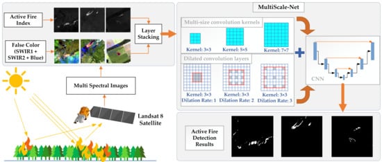
:Active fires are devastating natural disasters that cause socio-economical damage across the globe. The detection and mapping of these disasters require efficient tools, scientific methods, and reliable observations. Satellite images have been widely used for active fire detection (AFD) during the past years due to their nearly global coverage. However, accurate AFD and mapping in satellite imagery is still a challenging task in the remote sensing community, which mainly uses traditional methods. Deep learning (DL) methods have recently yielded outstanding results in remote sensing applications. Nevertheless, less attention has been given to them for AFD in satellite imagery. This study presented a deep convolutional neural network (CNN) “MultiScale-Net” for AFD in Landsat-8 datasets at the pixel level. The proposed network had two main characteristics: (1) several convolution kernels with multiple sizes, and (2) dilated convolution layers (DCLs) with various dilation rates. Moreover, this paper suggested an innovative Active Fire Index (AFI) for AFD. AFI was added to the network inputs consisting of the SWIR2, SWIR1, and Blue bands to improve the performance of the MultiScale-Net. In an ablation analysis, three different scenarios were designed for multi-size kernels, dilation rates, and input variables individually, resulting in 27 distinct models. The quantitative results indicated that the model with AFI-SWIR2-SWIR1-Blue as the input variables, using multiple kernels of sizes 3 × 3, 5 × 5, and 7 × 7 simultaneously, and a dilation rate of 2, achieved the highest F1-score and IoU of 91.62% and 84.54%, respectively. Stacking AFI with the three Landsat-8 bands led to fewer false negative (FN) pixels. Furthermore, our qualitative assessment revealed that these models could detect single fire pixels detached from the large fire zones by taking advantage of multi-size kernels. Overall, the MultiScale-Net met expectations in detecting fires of varying sizes and shapes over challenging test samples.
1. Introduction
Fire is one of the most devastating natural hazards, causing significant damage to human property and infrastructure [1]. In recent years, forest fires have had irreversible effects around the world, such as the recent fires in Canada (2016) [2], Australia (2019) [3], and California (2020) [4]. According to the Food and Agriculture Organization (FAO) report, in 2015 about 98 million hectares of forest were affected by fire. These forests were mainly in tropical regions, where fire engulfed at least 4% of the total forest area [5]. In 2018, a massive fire in California covering approximately 18,000 km2 killed 100 people and caused financial damage worth nearly USD 2 billion [6]. The accident happened again in 2020 in the same state, and burned approximately 17,000 km2 [7]. Such catastrophic and deadly fires frequently occur around the world. One of the key ways to control and monitor fires is to pinpoint their exact location, which can play a significant role in fire extinguishing operations. Using images/videos from terrestrial/aerial/satellite systems and implementing computer vision techniques such as image/video processing can be one of the best means for mapping fire extent [8,9,10].
Terrestrial-based systems are appropriate tools for early fire detection, which use optical and infrared (IR) cameras [11]. However, due to these systems’ lack of global coverage, satellite datasets covering almost the entire Earth to monitor active fires are one of the best alternative options. Various spaceborne sensors have been used for AFD [12]. In the past decade, the earth observations (EO) from two multispectral imaging sensors, namely a moderate resolution imaging spectroradiometer (MODIS) and a visible infrared imaging radiometer suite (VIIRS), have been frequently employed for AFD [13]. The VIIRS sensor on the Suomi National Polar-orbiting Partnership (S-NPP) satellite incorporates fire-sensitive channels, including a dual-gain high-saturation temperature channel at 4 µm, enabling AFD and characterization [14]. For example, Schroeder et al. [15] implemented and validated an algorithm for AFD using middle/thermal IR (M/TIR) bands of VIIRS images with 375 m of spatial resolution. Their results showed that VIIRS 375 m datasets could provide more coherent fire maps than MODIS 1 km fire products. Terra and Aqua satellites carry MODIS sensors as part of the National Aeronautics Space Administration (NASA) EO systems. These sensors have a revisit time of 1–2 days and capture data in 36 spectral bands ranging in wavelengths from 0.4 to 14.4 µm and at varying spatial resolutions (2 bands at 250 m, 5 bands at 500 m, and 29 bands at 1 km) [16]. Thanks to their daily temporal resolution, they play a crucial role in thermal sensing of land surface [17] and AFD [18]. For instance, Giglio et al. [17] validated the Collection 5 and 6 Terra MODIS fire products. They deliberated the modifications of Collection 6 compared to its previous version. Additionally, Parto et al. [18] employed a change detection approach to investigate the significant changes in forest features using the MODIS Normalized Difference Vegetation Index (NDVI) and thermal bands for real-time fire detection. Moreover, He et al. [19] proposed a method to eliminate the solar radiation and thermal path radiance received by the MODIS observations in the MIR band. The results demonstrated a reduction in errors associated with AFD.
Geostationary satellites are another widely used EO source for AFD and monitoring [20]. They have a high temporal but low spatial resolution. Himawari-8, a new generation of Japanese geostationary weather satellites operated by the Japan Meteorological Agency, has been used for AFD tasks. For example, Jang et al. [21] proposed a threshold-based forest fire detection algorithm based on Himawari-8 datasets over South Korea. Forest fire candidate pixels were initially identified, then the false alarms were removed using the random forest model followed by a post-processing phase. The results indicated the better capability of the suggested framework against the previous methods. Furthermore, Xie et al. [22] presented a spatiotemporal contextual model (STCM) for forest fire detection using Himawari-8 data. The results revealed the higher accuracy of the proposed method compared to the traditional contextual and temporal algorithms.
One of the essential purposes of fire control is to detect the accurate location and extent of the fire. Despite the widespread use of the abovementioned satellites, they have a coarse spatial resolution that causes uncertainty in AFD. Thus, spaceborne sensors with a higher spatial resolution, such as Landsat-8, should be used. Recently, many algorithms have been developed for AFD using Landsat-8 images [23]. AFD algorithms for the Advanced Spaceborne Thermal Emission and Reflection Radiometer (ASTER) sensor were the basis for developing the first fire detection methods in Landsat images [24]. In Landsat images, the probability of saturation of the pixels around the fire is relatively high, especially where highly reflective surfaces such as buildings are present. However, this problem was partially offset in Landsat-8 [15]. In the last five years, three AFD algorithms have been developed by Schroeder et al. [25], Murphy et al. [26], and Kumar et al. [24], yielding satisfactory results. The first two used thresholds on the reflectance of the SWIR1, SWIR2, and NIR bands, separately considering the day and night data. In contrast, the third algorithm used the Red band instead of the NIR. It should also be noted that these thresholds were determined with a series of statistical tests on a large number of fire pixels used to detect pixels with a very high fire probability.
Machine learning methods, in particular deep learning (DL), have been successfully applied in solving challenging tasks such as regression and classification problems [27,28], object detection [29], and semantic segmentation [30]. Many instances of implementing DL methods for AFD in unmanned aerial vehicles (UAVs) and terrestrial datasets [13]. However, only a few studies have focused on using these methods for AFD in satellite imagery [31,32]. Most previous AFD algorithms in satellite imagery have been based on fixed thresholds, contextual methods, multi-temporal approaches, and non-thermal IR methods using multi-sensor data [12]. These methods’ main problem is their low generalizability in complex terrain and illumination conditions. One of the main reasons for not using DL methods for AFD in satellite imagery in previous studies was the lack of a suitable dataset.
Thanks to the release of the large-scale dataset for AFD by de Almeida et al. [33], this paper proposed a deep encoder–decoder network, namely “MultiScale-Net”, for pixel-level localization of active fire in Landsat-8 imagery. This study developed a high-performance CNN architecture for AFD to identify individual fire pixels and even single ones detached from a large fire zone. In MultiScale-Net, we used convolution kernels with different sizes and dilated convolution layers (DCLs) with varying dilation rates to solve the challenges associated with changing the fire’s size and shape. The contributions of the present study are as follows:
- Developing a novel DL network for multi-scale AFD based on an efficient, sophisticated CNN architecture.
- Introducing a new index for AFD to improve MultiScale-Net performance in extracting high-level features.
- Using convolution layers with multi-size kernels and different dilation rates to facilitate multi-scale AFD.
- Assessing the performance of the proposed network using test samples with some challenges such as multi-size/shape fires (e.g., large fire zones alongside strip-shaped/single-pixel fires).
2. Remote Sensing Imagery
2.1. Landsat-8 Active Fire Dataset
A new large-scale dataset for AFD was recently published by De Almeida et al. [33]. This dataset contained image patches of 256 × 256 pixels, depicting the wildfires in several locations around the world, and was extracted from the Landsat-8 images from August to September 2020. The patches are 10-band, 16-bit TIFF images, with channels b1 to b11 excluding b8 (panchromatic channel) with 30 m of spatial resolution. Since all these patches have the same size, i.e., 256 × 256 pixels, the size of each image patch on the ground is 7680 by 7680 m. Three algorithms explained in detail in the references [24,25,26] produced the corresponding ground truth datasets. We selected the intersection between the three generated ground truths. As suggested in [33], we only used the SWIR2, SWIR1, and Blue bands in this study (Figure 1).
There was a significant class imbalance between fire and non-fire pixels in the dataset, with approximately 99% of the pixels being non-fire. We chose patches with the highest fire pixels compared to the most imbalanced samples in the dataset. Finally, 144 image patches were selected from the available dataset and split into 70% for training and validation (100 image patches) and 30% for testing (44 image patches). Test samples were selected considering the most significant challenges of AFD, such as changes in the size and shape of the fire in the image scene, the presence of clouds, and single fire pixels detached from the fire area. The training samples were from all five continents (Asia, Europe, Africa, Oceania, and the Americas) to adapt MultiScale-Net with different geographical, climatic, atmospheric, and illumination conditions.
2.2. Data Augmentation
Data augmentation is essential for training a DL network to improve generalization and reduce overfitting, especially when labeled or training data is limited [34]. There are many ways to reinforce training samples, one of the most popular of which is the flipping method. Using this method, the network will become resistant to the changes in direction and rotation. This augmentation method is easy to implement and has proven helpful in datasets such as CIFAR-10 and ImageNet [35]. In this study, we used horizontal, vertical, and horizontal-vertical flipping. As a result, the training samples quadrupled to 400 image patches.
3. Deep Multiple Kernel Learning
The proposed architecture is an efficient CNN for spectral-spatial feature extraction from remote sensing images. Moreover, an innovative index was used to extract semantic features related to active fire in the network inputs. A simple data augmentation technique was also used to compensate for the lack of training samples. According to Table 1, several configurations were considered based on different network parameters. For example, B3K35D1 represents a case where we used three bands, two kernels with sizes 3 and 5, and a dilation rate of 1. In total, we defined 27 different configurations. Figure 2 shows the scenarios experimented on within this study.
3.1. Active Fire Index
Fire detection methods are mainly based on the analysis of thermal and spectral bands. Previous research [25] shows that Band 7 of the Landsat-8 sensor (i.e., SWIR2) is sensitive to fire radiation. In this study, an index for AFD was proposed, namely Active Fire Index (AFI), which can be computed using Equation (1).
where and represent the SWIR2 and Blue values in Landsat-8 images, respectively. According to Equation (1), three essential characteristics of AFI can be stated. Firstly, it is appropriate to highlight the fire from the background (see Figure 3) due to its high reflectance in SWIR2 and relatively low reflectance in the Blue spectral ranges. The second characteristic is removing smoke, a disturbing factor in AFD often present in the fire region in satellite images. Smoke has a high reflectance in the Blue spectral range while slightly reflecting in the SWIR2 band [36]. This difference in spectral behavior causes the AFI value to be low in the smoke-contaminated pixels (Figure 3, third row). The third is the removal of possibly present clouds in the image scene. The presence of clouds is one of the challenging problems in AFD [37]. The most common method to deal with this problem is cloud masking. Improper cloud masking can hide actual fire pixels at the cloud boundary [38]. Due to the higher reflectance of the cloud in the visible spectral region compared to SWIR2 [39], the AFI value is low in the cloud-contaminated pixels (Figure 4).
Although the proposed index is computationally straightforward, it has an excellent performance in separating the active fire from the background (see Figure 3). However, it has an undesirable performance on a few occasions, e.g., when bright non-fire objects have a high reflectance in the SWIR2 and a low reflectance in the Blue spectra (Figure 4, second row).
3.2. Network Architecture
The proposed method’s architecture is a fully convolutional framework in which the output is a pixel-by-pixel map with the same size as the input image. The proposed network differs from previous AFD architectures in satellite imagery [33], which used a simple U-Net. In the proposed architecture, a combination of convolution features with different kernel sizes was implemented for improving the accuracy of AFD. The idea was to use features extracted at various scales from multi-size kernels to provide local and general properties. The feature maps of the lower-level encoder layers retained more spatial details, leading to more precise boundaries. Higher-level features were extracted in the deeper convolution layers. Subsequently, the max-pooling layers down-sampled the extracted feature maps in the encoder part.
In contrast, the decoder part up-sampled the feature maps by deconvolution layers. Concatenation links transferred the extracted feature maps to the corresponding decoder from the encoder. This operation resulted in the generation of more meaningful features. In addition to kernels with different sizes, DCLs were employed to extract multi-scale fires in conditions with variable sizes in the image scene. Dilated convolutions add a new parameter to convolutional layers known as the dilation rate. This parameter introduces a distance between values in a convolution kernel. A 3 × 3 kernel with a dilation rate of 2 has the same field of view as a 5 × 5 kernel but removes every other column and row from a 5 × 5 kernel. In this study, dilation rates of 1, 2, and 3 were tested in the second convolution layer in each block (the dilation rate in the first layer of each block was considered constant 1). Our proposed method has the following characteristics:
- The proposed DL architecture has a network depth of 5 (network length).
- It takes advantage of a new approach that includes convolutional kernels with different sizes for the training process.
- DCLs with different dilation rates are employed.
- Batch normalization and dropout are used, which play an essential role in preventing over-fitting [40].
- A binary cross-entropy loss function is utilized. Moreover, the “glorot_uniform” method initializes the network [41].
Figure 5 shows one of the most complex configurations used in MultisScale-Net. Different configurations based on using DCLs with different dilation rates in the second layer, simultaneous employment of kernels with different sizes, and different scenarios of network input variables were examined (see Figure 2).
The proposed network consists of an encoder part and a decoder part. The encoder part carries out five convolution blocks. It consists of repeated applications of two 3 × 3, 5 × 5, 7 × 7 convolutional layers with two paddings. Each convolution follows a batch normalization (BN) layer and rectified linear units (ReLU) activation function. Moreover, each convolution block is followed by 2 × 2 max-pooling for down-sampling with the stride of 2. The number of feature channels is doubled after each block. The decoder branch corresponds to the encoder and consists of four transposed convolution layers. Every block in the decoder branch consists of a 3 × 3 deconvolution with the stride of 2, a concatenation with the corresponding feature maps from the encoder, and two 3 × 3, 5 × 5, 7 × 7 convolutions followed by ReLU activation and BN layer. The number of feature channels is halved after each up-sampling process. A 1 × 1 convolution with a Softmax activation function is employed as a classifier at the final layer, followed by a binary cross-entropy (BCE) loss function.
The BCE loss function compares each predicted probability with the actual class’s output, 0 or 1 (in binary classification). The calculated score then determines the probabilities based on the distance from the expected value. This score shows how the predicted values are close to or far from the actual value. In order to minimize this score in the training process, one should update the network parameters with high accuracy [39]. For binary segmentation, the BCE is used, which is defined as follows:
that is the probability of fire class, and is the probability of non-fire class. Then denotes the number of pixels, and is the pixel label.
All scenarios were designed and trained using the Keras library on the Google Colab platform, utilizing a Tesla T4 GPU with a batch size of 15 for 200 epochs. Moreover, the adaptive moment estimation (Adam) method was used to optimize the trainable network parameters. In this method, the learning rate, beta-1, beta-2, and epsilon were chosen as , , and respectively.
Table 2 shows the output size, kernel sizes, activation functions, and different types of concatenations in the encoder and decoder part of MultiScale-Net, respectively. The MultiScale-Net employs three types of concatenations that combine features with high abstraction ability, and they are as follows:
- Intra-block concatenations fuse feature maps from the first and second convolution layers with the same kernel size in each block.
- Inter-block concatenations fuse feature maps generated by convolution layers with varying kernel sizes from distinct blocks.
- Inter-branch concatenations fuse feature maps from the encoder and the decoders’ transposed convolution blocks.
3.3. Accuracy Metrics
In the field of AFD, due to the destructive nature of fire, determining the exact extent of the fire and recognizing the fire pixels in Landsat-8 satellite images is essential. Therefore, the criteria used to assess accuracy are very important. In this study, four accuracy criteria—Precision (P), Sensitivity (S), F1-score (F), and intersection over union (IoU or I)—were considered. The precision, also called the correctness in the remote sensing literature, is the ratio of predicted fire pixels that are actual fire. The sensitivity, also called recall, is the ratio of actual fire pixels correctly detected. The F1-score is defined as the harmonic mean of the two criteria, precision and sensitivity, the optimality of which indicates the balance between these two criteria [42]. However, due to the possibility of imbalance between fire and non-fire classes, additional criteria need to be calculated to understand the model’s actual performance, as precision can be misleading in an unbalanced dataset. Therefore, we also used IoU, known as Jaccard Index (JI) [43]. The IoU metric is a standard criterion for semantic segmentation, which indicates the ratio of correctly segmented pixels as fire to total numbers of ground reference pixels. The criteria described above can be obtained from the following equations (TP: true positive, FP: false positive, and FN: false negative):
where TP represents the number of fire pixels in the fire class, FP represents the number of fire pixels in the non-fire class, and FN indicates the number of non-fire pixels in the fire class.
4. Results and Discussion
In this study, due to the usage of many different configurations for AFD, the accuracy criteria in different scenarios were first examined. Then, the visual outputs of the best models were displayed.
4.1. Accuracy Assessment of AFD
The statistical accuracy assessment of the AFD with 27 models using four accuracy metrics is summarized in Table 3. Based on the input variables (i.e., B1, B3, and B4) that are mentioned in Table 1, we evaluated the accuracy criteria in three scenarios:
- B3 scenario: The highest precision, sensitivity, F1-score, and IoU are associated with the K3D1 (P = 95.71%), K35D3 (S = 93.93%), K35D1 (F = 91.45%), and K35D1 (I = 84.24%) models, respectively, in this scenario.
- B4 scenario: In this scenario, the best precision, sensitivity, F1-score, and IoU are related to the K3D2 (P = 92.51%), K35D1 (S = 92.52%), K357D2 (F = 91.62%), and K357D2 (I = 84.54%) models, respectively.
- B1 scenario: In this scenario, the best precision, sensitivity, F1-score, and IoU are associated with the K35D1 (P = 94.5%), K357D2 (S = 92.49%), K357D2 (F = 91.11%), and K357D2 (I = 83.67%) models, respectively.
These statistical results show that the proposed method extracts and integrates informative high-level features from the network inputs and thus produces fire masks that are very similar to ground truth in all scenarios. The simultaneous use of kernels with different sizes in MultiScale-Net has resulted in satisfactory consequences because ten models used multi-size kernels out of the top 12 models. Moreover, dilation rates of 1 and 2 had better impacts than 3. In other words, eleven models out of the top 12 models used dilation rates of 1 or 2. Further analysis about the influence of multi-size kernels and dilation rate in AFD by MultiScale-Net are assessed in Section 4.5.
4.2. Qualitative Evaluation of MultiScale-Net
According to Equation (6), the IoU is equal to 1 if both FP and FN are equal to zero. In other words, the DL network should not have any misdetection. Therefore, IoU is a strict metric, and for visual output maps, the models with the highest IoU were selected (i.e., B1K357D2, B3K35D1, and B4K357D2). The binary output maps of the selected models are shown in Figure 6. All three models have detected active fire locations with relatively satisfactory accuracy. There is no significant difference between their outputs. The slight differences were frequently seen in locations where the extent of the fire ranges from a wide area to a single pixel. In such circumstances, the B4K357D2 outperformed the other models, and the number of FNs in this model’s outputs was reduced (e.g., samples (a), (i), and (j) in Figure 6). Furthermore, all three models chosen from the MultiScale-Net perform better in the situation of fire strips than single-pixels detached from the fire zones (e.g., samples (d), (e), and (h) in Figure 6). However, the MultiScale-Net is robust enough to alter the size and shape of the fire in the image scene.
The sample (j) (Figure 6) had more visual distinction between fire and background than the other samples, with fewer fire-like objects in the image scene. The number of FPs in this sample’s output map of B1K357D2, B3K35D1, and B4K357D2 was 3, 2, and 0, respectively. In contrast, all three models’ output maps contained many FN pixels. Therefore, it can be argued that, while decreasing the complexity of image conditions for AFD has resulted in fewer false alarms (i.e., FP pixels), it has also resulted in the MultiScale-Net being negligent. Many fire pixels, particularly those on the boundary between fire and background, were misclassified as non-fire (i.e., FN pixels) by the MultiScale-Net.
Most AFD errors happened in the large fire zones’ peripheral pixels. However, in rare situations, non-fire pixels surrounded by a large fire region were detected as fire pixels by the MultiScale-Net (i.e., FP pixels) (sample (b) in Figure 6). This misdetection is most likely owing to the extremely high temperature of the surrounding fire pixels (i.e., TP pixels) and their influence on the spectral reflectance of the inside pixels (i.e., FP pixels). In certain instances, the fire zone’s center may be incorrectly classified as non-fire (see Figure 7). In some test samples, the pixel saturation issue was seen visually, so that it also involved producing ground truth in this dataset (i.e., the algorithms developed in [24,25,26]). In Figure 7, the digital number values of pixels in the SWIR2 band, seen in green, are minimal or even zero in some of these pixels. As mentioned in the introduction, one of the sensitive bands for AFD is SWIR2, and its value is zero in the green pixels in this image. Visually, and given the fire extent in this image, these pixels might be saturated. Again, the B4K357D2 model is more similar to the ground truth.
It should be mentioned that given the nature of fire, especially its appearance in satellite images with limited spatial resolution and the significant effect of the Earth’s atmosphere, such visual interpretations may be accompanied by inaccuracy. Figure 8 shows minor differences between network predictions in different models in another test sample of the dataset. The primary distinction was where the two fire zones meet. The B4K357D2 model generated the closest map to the ground truth, although there was a gap between the two fire zones in the other two cases.
4.3. Qualitative Assessment of MultiScale-Net in Severe Cloud Condition
One of the significant challenges in AFD is the presence of many clouds in the image scene. As a result, in some studies, cloud masking was applied prior to fire detection. Moreover, the few fire pixels make it challenging to identify them in the image. In this study, however, these challenging issues were considered (i.e., severe cloud conditions and the low number of fire pixels) to assess the performance of the best-selected models from the previous steps. Figure 9 shows that the two models, B4K357D2 and B3K35D1, have the same performance and are somewhat different from ground truth, but the B1K357D2 model performs differently from the previous two models with more disagreement with ground truth. It can be seen that it is visually difficult to distinguish the fire pixels from non-fire, and there is much uncertainty. All three models have false positive (FP) pixels; the pixels are detected fire but are actually non-fire in the ground truth.
Both models, B3K35D1 and B4K357D2, detected a single pixel of fire surrounded by multiple cloud pixels, as shown in Figure 10, while the B1K357D2 model was unable to do so. This result demonstrates that concurrent use of multi-size kernels and selecting the appropriate input scenario (i.e., B3 and B4) in the MultiScale-Net could extract the spectral-spatial features associated with active fire, allowing even a single pixel of fire surrounded by non-fire pixels to be correctly detected.
4.4. Effect of Adding AFI to the three Landsat-8 Bands
This study presented a new indicator, AFI, for AFD in Landsat-8 imagery. The B4 scenario offered the best F1-score and IoU in which the AFI and the three Landsat-8 bands were stacked. Of course, several kernels with different sizes or different dilation rates may have influenced the obtained results. Thus, the results in different configurations of each scenario (B1, B2, and B3) were averaged.
As is clear from Table 3, the highest average values for IoU, F1-score, and sensitivity were associated with the B4 scenario. However, in the case of the precision criterion, the highest mean value was associated with the B3 scenario. Even the average precision in the B1 scenario was better than in B4. Since the best accuracy in B1 was about 2% higher than in B4, the average value may have increased due to this high maximum value. Therefore, the number of TP, FP, and FN pixels should be analyzed more attentively. As is clear from Figure 11, the number of FN pixels in the B4 scenario was less than the other two cases, while the number of FP pixels in the B3 scenario was less than the others. In the field of AFD, FN pixels are fire pixels identified as non-fire by the network. FN pixels can be dangerously misleading in terms of fire extinguishing operations. However, FP pixels are non-fire pixels identified as fire by the network, which is considered a “false alarm” in crisis management.
On the other hand, the addition of AFI increased the number of TP pixels in the B4 scenario compared to the other two scenarios. The lower precision in B4 compared with the B3 scenario was due to the higher FP pixels. Nevertheless, in criteria such as sensitivity, where the FN pixels play the primary role instead of FPs (see Equation (4)), the B4 scenario offered outstanding performance. Moreover, in most of the test samples, the B4 scenario was more in line with ground truth (as in Figure 7 and Figure 8), but in severe cloudy conditions with a few fire pixels in the scene, there was no difference in the results (as in Figure 9 and Figure 10). Therefore, our innovative index helped separate active fire from the background by stacking it with three other bands (SWIR2, SWIR1, and Blue). Although using the AFI as the sole input of the network did not lead to better results than the other two scenarios, it led to fewer FP pixels than in B4.
4.5. Effect of Multi-Size Kernels and DCLs
Multi-size kernels have achieved decent results in building extraction [44] and cloud/cloud shadow segmentation [45]. This study used this technique to extract the fire’s extent better and discriminate between fire and other objects with high reflectivity in the SWIR2 band. According to Table 3, all the 12 best models utilized multi-size kernels, except for two models. These two cases had the best precision, while the other ten models had the best scores in the other criteria. One of the test samples was selected to visually analyze the AFD performance of the multi-size kernels. Considering a specific input variables scenario (i.e., B4) and a constant dilation rate (i.e., D2), the MultiScale-Net output was compared in regards to multi-size kernels (see Figure 12). One of the challenges in AFD is the change in the fire scale in an image scene where the fire size varies from a few pixels to large clusters in different parts of the image. As is clear in Figure 12, K357 outperformed the other two kernel scenarios (i.e., K3 and K35) and was relatively robust to changes in fire size.
The DCLs were used in deep neural networks to extract features with different scales. In this study, DCLs with dilation rates of 1, 2, and 3 were used to enhance AFD and deal with the challenge associated with fire size change. As is clear from Table 3, only one of the top models used a dilation rate of 3. Of the remaining eleven top models, six had a dilation rate of 2, while the other five had a dilation rate of 1. However, it should be noted that increasing the dilation rate from 1 to 2 improved accuracy in some cases but not always.
The number of FPs, FNs, and TPs in different scenarios was investigated to evaluate further the influence of multi-size kernels and DCLs on the performance of MultiScale-Net (Figure 13). As shown in Figure 13, K35D1, K3D1, and K35D2 had the lowest FPs in the B1, B3, and B4 input variables scenarios, while K357D2, K35D3, and K35D1 had the lowest FNs, respectively. As a result, it can be approximately deduced that using multi-size kernels, particularly two kernels with sizes of 3 and 5 (i.e., K35), produced minor defects in AFD compared to a kernel with a constant size of 3. However, in higher dilation rates (especially rate 3), DCLs did not significantly increase AFD accuracy. Although, in some circumstances, the dilation rate of 2 effectively reduced FPs and FNs. These outcomes agreed with the statistical results in Section 4.1 (see Table 3).
4.6. Comparison Analysis
Previous studies in AFD have primarily relied on thresholding certain spectral bands and the analysis of image pixel statistics, with just a few studies employing deep CNNs due to the lack of a massive training dataset. These networks have many trainable parameters that require many labeled samples for proper estimation. To our knowledge, De Almeida et al. [33] provided the first large-scale dataset for AFD. Our study’s primary distinction was in developing a new efficient CNN architecture and experimenting with different network input types. Our main objective was to create a high-performance CNN architecture for AFD that is more robust against fire size and shape.
However, the main goal of their research was to prepare and publish a large-scale dataset for AFD through DL algorithms and to demonstrate the potential of these methods for AFD. Their study relied only on the U-Net, one of the most widespread and straightforward CNNs available for segmentation and classification tasks in the remote sensing community. On the other hand, our study employed convolution kernels with multiple sizes and DCLs with varied rates. The feature maps produced from the multi-scale convolution layers were concatenated into each convolution block to provide high-level features that allowed the MultiScale-Net to detect active fires with reasonable accuracy. Furthermore, our proposed method was resistant to active fire size change due to multi-size kernels and, in some instances, DCLs with varying rates. U-Net, on the other hand, lacks all of these characteristics.
Moreover, adding the introduced AFI to the Landsat-spectral bands as inputs to the models resulted in the extraction of more informative features and enhanced network performance in AFD. De Almeida et al. [33] considered two scenarios for U-Net input variables, including three and ten Landsat-8 spectral bands. In contrast, our study considered three scenarios for network input types (i.e., B1, B3, and B4). Another notable distinction between the two studies is using different CNN training and testing scenarios. The U-Net 10c (ten bands of Landsat-8 image as input), U-Net 3c (three bands of Landsat-8 image as input), and U-Net 3c light (similar to U-Net 3c, but with just a quarter of the number of convolution kernels in each layer) were utilized in their study. Moreover, as ground truths data, binary fire masks based on the three sets of conditions described in [24,25,26] were employed individually, with voting and intersection between them (five types in total), resulting in 15 different training scenarios. The output maps were also compared to the manually annotated data during the testing phase. However, the MultiScale-Net was evaluated in 27 different scenarios in terms of network architecture (such as the simultaneous use of kernels of different sizes -K3, K35, K357- and DCLs with variable dilation rates -D1, D2, D3-) and input variables (B1, B3, and B4).
5. Conclusions
Active fires are among the most harmful hazards impacting wildlife and ecosystems. With the development of artificial intelligence technology, DL methods have made great strides in computer vision and image processing. This study proposed the deep CNN “MultiScale-Net” for AFD using Landsat-8 imagery. The developed CNN benefited from two significant differences compared with the early DL networks: (1) The employment of convolution kernels with different sizes simultaneously in each convolution layer; (2) The utilization of dilated convolution layers with different dilation rates. The main advantages of the proposed CNN can be summarized in three aspects:
- Geographically diverse training samples from five different study areas across the world made the network robust against different geographical and illumination conditions.
- MultiScale-Net showed satisfactory performance in extracting different-sized fires in the challenging test samples.
- This study proposed AFI, a new innovative indicator for AFD, derived from the SWIR2 and Blue bands. Multiscale-Net uses AFI as an input feature to increase accuracy.
Scenario-based analyses of quantitative and qualitative experimental results were carried out. A total of 27 models were examined based on changing three scenarios: input variables (B1, B3, and B4), multi-size kernels (K3, K35, and K357), and dilation rates (D1, D2, and D3). Most of the best models were the ones that used multi-size kernels and stacked AFI with three Landsat-8 bands as the input features. In some samples, using a dilation rate of 2 improved the quantitative results, but 3 was inefficient. The highest precision, sensitivity, F1-score, and IoU scores were 95.71%, 93.93%, 91.62%, and 84.54%, respectively, when testing on the 40 samples. Among the input feature scenarios, B4 (AFI stacked with three Landsat-8 spectral bands) had the highest mean sensitivity, F1-score, and IoU scores of 89.66%, 90.57%, and 82.79%, respectively. This scenario had the least FN pixels among the other scenarios, which is a desirable asset for fire extinguishing operations because this misdetection can cause irreversible damage. Qualitative investigations also revealed that using multi-size kernels makes the MultiScale-Net more robust against changes in patterns and size of the active fire in the image. The multi-size kernels in the B4 scenario enhanced the MultiScale-Net performance where major fire zones meet. The MultiScale-Net was tested in samples containing clouds and single fire pixels detached from major fire zones, with satisfactory outcomes.
This study was a new step in using DL techniques for AFD in satellite imagery, which has received less attention in previous studies. The findings of this study can be used to manage and control fires effectively and reduce their damage. Due to the independence of our proposed method on the thermal bands, future studies could investigate the potential of Sentinel-2 data for AFD with higher spatial and temporal resolution. Moreover, the processing time of the proposed method can be evaluated in cloud platforms such as Google Earth Engine (GEE).
Author Contributions
Conceptualization, A.R. and R.S.-H.; methodology, A.R., S.A. and A.Z.; software, A.R., S.A. and A.Z.; formal analysis, S.H.; investigation, A.R., R.S.-H. and M.A.-N.; writing—original draft preparation, A.R.; writing—review and editing, A.R., R.S.-H., S.H. and M.A.-N.; visualization, R.S.-H., M.A.-N., S.A. and A.Z.; supervision, R.S.-H.; project administration, R.S.-H. and S.H. All authors have read and agreed to the published version of the manuscript.
Funding
This research received no external funding.
Institutional Review Board Statement
Not applicable.
Informed Consent Statement
Not applicable.
Data Availability Statement
Publicly available datasets were analyzed in this study. These datasets can be found here: [https://github.com/pereira-gha/activefire] (accessed on 17 October 2021).
Acknowledgments
The authors would like to present their appreciation to de Almeida et al. for providing and publishing the unique and valuable dataset for the remote sensing community.
Conflicts of Interest
The authors declare no conflict of interest.
References
- Seydi, S.T.; Hasanlou, M.; Chanussot, J. DSMNN-Net: A Deep Siamese Morphological Neural Network Model for Burned Area Mapping Using Multispectral Sentinel-2 and Hyperspectral PRISMA Images. Remote Sens. 2021, 13, 5138. [Google Scholar] [CrossRef]
- Lalani, N.; Drolet, J.L.; McDonald-Harker, C.; Brown, M.R.G.; Brett-MacLean, P.; Agyapong, V.I.O.; Greenshaw, A.J.; Silverstone, P.H. Nurturing Spiritual Resilience to Promote Post-Disaster Community Recovery: The 2016 Alberta Wildfire in Canada. Front. Public Health 2021, 9, 682558. [Google Scholar] [CrossRef] [PubMed]
- Seydi, S.T.; Akhoondzadeh, M.; Amani, M.; Mahdavi, S. Wildfire Damage Assessment over Australia Using Sentinel-2 Imagery and MODIS Land Cover Product within the Google Earth Engine Cloud Platform. Remote Sens. 2021, 13, 220. [Google Scholar] [CrossRef]
- Keeley, J.E.; Syphard, A.D. Large California Wildfires: 2020 Fires in Historical Context. Fire Ecol. 2021, 17, 22. [Google Scholar] [CrossRef]
- FAO. Global Forest Resources Assessment 2020—Key Findings; FAO: Rome, Italy, 2020. [Google Scholar]
- Gin, J.L.; Balut, M.D.; Der-Martirosian, C.; Dobalian, A. Managing the Unexpected: The Role of Homeless Service Providers during the 2017–2018 California Wildfires. J. Community Psychol. 2021, 49, 2532–2547. [Google Scholar] [CrossRef]
- Ball, G.; Regier, P.; González-Pinzón, R.; Reale, J.; Van Horn, D. Wildfires Increasingly Impact Western US Fluvial Networks. Nat. Commun. 2021, 12, 2484. [Google Scholar] [CrossRef]
- Toulouse, T.; Rossi, L.; Celik, T.; Akhloufi, M. Automatic Fire Pixel Detection Using Image Processing: A Comparative Analysis of Rule-Based and Machine Learning-Based Methods. Signal Image Video Process. 2016, 10, 647–654. [Google Scholar] [CrossRef] [Green Version]
- Martinez-de Dios, J.R.; Arrue, B.C.; Ollero, A.; Merino, L.; Gómez-Rodríguez, F. Computer Vision Techniques for Forest Fire Perception. Image Vis. Comput. 2008, 26, 550–562. [Google Scholar] [CrossRef]
- Valero, M.M.; Rios, O.; Pastor, E.; Planas, E. Automated Location of Active Fire Perimeters in Aerial Infrared Imaging Using Unsupervised Edge Detectors. Int. J. Wildland Fire 2018, 27, 241–256. [Google Scholar] [CrossRef] [Green Version]
- Alkhatib, A.A.A. A Review on Forest Fire Detection Techniques. Int. J. Distrib. Sens. Netw. 2014, 10, 597368. [Google Scholar] [CrossRef] [Green Version]
- Wooster, M.J.; Roberts, G.J.; Giglio, L.; Roy, D.P.; Freeborn, P.H.; Boschetti, L.; Justice, C.; Ichoku, C.; Schroeder, W.; Davies, D.; et al. Satellite Remote Sensing of Active Fires: History and Current Status, Applications and Future Requirements. Remote Sens. Environ. 2021, 267, 112694. [Google Scholar] [CrossRef]
- Barmpoutis, P.; Papaioannou, P.; Dimitropoulos, K.; Grammalidis, N. A Review on Early Forest Fire Detection Systems Using Optical Remote Sensing. Sensors 2020, 20, 6442. [Google Scholar] [CrossRef] [PubMed]
- Csiszar, I.; Schroeder, W.; Giglio, L.; Ellicott, E.; Vadrevu, K.P.; Justice, C.O.; Wind, B. Active Fires from the Suomi NPP Visible Infrared Imaging Radiometer Suite: Product Status and First Evaluation Results. J. Geophys. Res. Atmos. 2014, 119, 803–816. [Google Scholar] [CrossRef]
- Schroeder, W.; Oliva, P.; Giglio, L.; Csiszar, I.A. The New VIIRS 375m Active Fire Detection Data Product: Algorithm Description and Initial Assessment. Remote Sens. Environ. 2014, 143, 85–96. [Google Scholar] [CrossRef]
- Xiong, X.; Aldoretta, E.; Angal, A.; Chang, T.; Geng, X.; Link, D.; Salomonson, V.; Twedt, K.; Wu, A. Terra MODIS: 20 Years of on-Orbit Calibration and Performance. J. Appl. Remote Sens. 2020, 14, 1–16. [Google Scholar] [CrossRef]
- Giglio, L.; Schroeder, W.; Justice, C.O. The Collection 6 MODIS Active Fire Detection Algorithm and Fire Products. Remote Sens. Environ. 2016, 178, 31–41. [Google Scholar] [CrossRef] [Green Version]
- Parto, F.; Saradjian, M.; Homayouni, S. MODIS Brightness Temperature Change-Based Forest Fire Monitoring. J. Indian Soc. Remote Sens. 2020, 48, 163–169. [Google Scholar] [CrossRef]
- He, L.; Li, Z. Enhancement of a Fire-Detection Algorithm by Eliminating Solar Contamination Effects and Atmospheric Path Radiance: Application to MODIS Data. Int. J. Remote Sens. 2011, 32, 6273–6293. [Google Scholar] [CrossRef]
- Engel, C.B.; Jones, S.D.; Reinke, K. A Seasonal-Window Ensemble-Based Thresholding Technique Used to Detect Active Fires in Geostationary Remotely Sensed Data. IEEE Trans. Geosci. Remote Sens. 2021, 59, 4947–4956. [Google Scholar] [CrossRef]
- Jang, E.; Kang, Y.; Im, J.; Lee, D.-W.; Yoon, J.; Kim, S.-K. Detection and Monitoring of Forest Fires Using Himawari-8 Geostationary Satellite Data in South Korea. Remote Sens. 2019, 11, 271. [Google Scholar] [CrossRef] [Green Version]
- Xie, Z.; Song, W.; Ba, R.; Li, X.; Xia, L. A Spatiotemporal Contextual Model for Forest Fire Detection Using Himawari-8 Satellite Data. Remote Sens. 2018, 10, 1992. [Google Scholar] [CrossRef] [Green Version]
- Liu, Z.; Wu, K.; Jiang, R.; Zhang, H. A Simple Artificial Neural Network For Fire Detection Using LANDSAT-8 Data. Int. Arch. Photogramm. Remote Sens. Spat. Inf. Sci. 2020, 43, 447–452. [Google Scholar] [CrossRef]
- Kumar, S.S.; Roy, D.P. Global Operational Land Imager Landsat-8 Reflectance-Based Active Fire Detection Algorithm. Int. J. Digit. Earth 2018, 11, 154–178. [Google Scholar] [CrossRef] [Green Version]
- Schroeder, W.; Oliva, P.; Giglio, L.; Quayle, B.; Lorenz, E.; Morelli, F. Active Fire Detection Using Landsat-8/OLI Data. Landsat 8 Sci. Results 2016, 185, 210–220. [Google Scholar] [CrossRef] [Green Version]
- Murphy, S.W.; de Souza Filho, C.R.; Wright, R.; Sabatino, G.; Correa Pabon, R. HOTMAP: Global Hot Target Detection at Moderate Spatial Resolution. Remote Sens. Environ. 2016, 177, 78–88. [Google Scholar] [CrossRef]
- Ansari, M.; Homayouni, S.; Safari, A.; Niazmardi, S. A New Convolutional Kernel Classifier for Hyperspectral Image Classification. IEEE J. Sel. Top. Appl. Earth Obs. Remote Sens. 2021, 14, 11240–11256. [Google Scholar] [CrossRef]
- Ranjbar, S.; Zarei, A.; Hasanlou, M.; Akhoondzadeh, M.; Amini, J.; Amani, M. Machine Learning Inversion Approach for Soil Parameters Estimation over Vegetated Agricultural Areas Using a Combination of Water Cloud Model and Calibrated Integral Equation Model. J. Appl. Remote Sens. 2021, 15, 1–17. [Google Scholar] [CrossRef]
- Zhao, Z.-Q.; Zheng, P.; Xu, S.-T.; Wu, X. Object Detection With Deep Learning: A Review. IEEE Trans. Neural Netw. Learn. Syst. 2019, 30, 3212–3232. [Google Scholar] [CrossRef] [Green Version]
- Diakogiannis, F.I.; Waldner, F.; Caccetta, P.; Wu, C. ResUNet-a: A Deep Learning Framework for Semantic Segmentation of Remotely Sensed Data. ISPRS J. Photogramm. Remote Sens. 2020, 162, 94–114. [Google Scholar] [CrossRef] [Green Version]
- Vani, K. Deep Learning Based Forest Fire Classification and Detection in Satellite Images. In Proceedings of the 2019 11th International Conference on Advanced Computing (ICoAC), Chennai, India, 18–20 December 2019; pp. 61–65. [Google Scholar]
- Phan, T.C.; Nguyen, T.T. Remote Sensing Meets Deep Learning: Exploiting Spatio-Temporal-Spectral Satellite Images for Early Wildfire Detection. No. REP_WORK. 2019. Available online: https://Infoscience.Epfl.Ch/Record/270339 (accessed on 7 September 2020).
- de Almeida Pereira, G.H.; Fusioka, A.M.; Nassu, B.T.; Minetto, R. Active Fire Detection in Landsat-8 Imagery: A Large-Scale Dataset and a Deep-Learning Study. ISPRS J. Photogramm. Remote Sens. 2021, 178, 171–186. [Google Scholar] [CrossRef]
- Shorten, C.; Khoshgoftaar, T.M. A Survey on Image Data Augmentation for Deep Learning. J. Big Data 2019, 6, 60. [Google Scholar] [CrossRef]
- Wang, Y.; Pan, X.; Song, S.; Zhang, H.; Huang, G.; Wu, C. Implicit Semantic Data Augmentation for Deep Networks. Adv. Neural Inf. Process. Syst. 2019, 32, 12635–12644. [Google Scholar]
- King, M.D.; Platnick, S.; Moeller, C.C.; Revercomb, H.E.; Chu, D.A. Remote Sensing of Smoke, Land, and Clouds from the NASA ER-2 during SAFARI 2000. J. Geophys. Res. Atmos. 2003, 108, 8502. [Google Scholar] [CrossRef]
- Giglio, L.; Descloitres, J.; Justice, C.O.; Kaufman, Y.J. An Enhanced Contextual Fire Detection Algorithm for MODIS. Remote Sens. Environ. 2003, 87, 273–282. [Google Scholar] [CrossRef]
- Cadau, E.; Laneve, G. Improved MSG-SEVIRI Images Cloud Masking and Evaluation of Its Impact on the Fire Detection Methods. In Proceedings of the IGARSS 2008—2008 IEEE International Geoscience and Remote Sensing Symposium, Boston, MA, USA, 7–11 July 2008; Volume 2, p. II-1056. [Google Scholar]
- Ho, Y.; Wookey, S. The Real-World-Weight Cross-Entropy Loss Function: Modeling the Costs of Mislabeling. IEEE Access 2020, 8, 4806–4813. [Google Scholar] [CrossRef]
- Garbin, C.; Zhu, X.; Marques, O. Dropout vs. Batch Normalization: An Empirical Study of Their Impact to Deep Learning. Multimed. Tools Appl. 2020, 79, 12777–12815. [Google Scholar] [CrossRef]
- Glorot, X.; Bengio, Y. Understanding the Difficulty of Training Deep Feedforward Neural Networks. In Proceedings of the Thirteenth International Conference on Artificial Intelligence and Statistics, Sardinia, Italy, 13–15 May 31 2010; Volume 9, pp. 249–256. [Google Scholar]
- Chicco, D.; Jurman, G. The Advantages of the Matthews Correlation Coefficient (MCC) over F1 Score and Accuracy in Binary Classification Evaluation. BMC Genom. 2020, 21, 6. [Google Scholar] [CrossRef] [Green Version]
- Hamers, L. Similarity Measures in Scientometric Research: The Jaccard Index versus Salton’s Cosine Formula. Inf. Process. Manag. 1989, 25, 315–318. [Google Scholar] [CrossRef]
- Khoshboresh-Masouleh, M.; Alidoost, F.; Arefi, H. Multiscale Building Segmentation Based on Deep Learning for Remote Sensing RGB Images from Different Sensors. J. Appl. Remote Sens. 2020, 14, 1–21. [Google Scholar] [CrossRef]
- Khoshboresh-Masouleh, M.; Shah-Hosseini, R. A Deep Learning Method for Near-Real-Time Cloud and Cloud Shadow Segmentation from Gaofen-1 Images. Comput. Intell. Neurosci. 2020, 2020, 8811630. [Google Scholar] [CrossRef]
Figure 1.
(a–c) RGB, (b–d) False color (SWIR2, SWIR1, and Blue) of Landsat-8 images from the reference dataset.
Figure 1.
(a–c) RGB, (b–d) False color (SWIR2, SWIR1, and Blue) of Landsat-8 images from the reference dataset.

Figure 2.
Different scenarios based on the number of inputs, multi-size kernels, and DCLs with different dilation rates in MultiScale-Net for AFD.
Figure 2.
Different scenarios based on the number of inputs, multi-size kernels, and DCLs with different dilation rates in MultiScale-Net for AFD.

Figure 3.
AFI maps from several Landsat-8 images. Each row illustrates a sample image in the dataset.
Figure 3.
AFI maps from several Landsat-8 images. Each row illustrates a sample image in the dataset.

Figure 4.
The performance of the AFI for AFD in cloudy scenes. Each row represents a sample image in the dataset with the red circles indicating the approximate fire range.
Figure 4.
The performance of the AFI for AFD in cloudy scenes. Each row represents a sample image in the dataset with the red circles indicating the approximate fire range.

Figure 5.
The proposed network for AFD. “Conv2d (k × k)” shows the convolutional kernel with the size of k × k; “Batch Norm.” denotes batch normalization; “ReLU” denotes the rectified linear units. “Dlr” denotes dilation rate.
Figure 5.
The proposed network for AFD. “Conv2d (k × k)” shows the convolutional kernel with the size of k × k; “Batch Norm.” denotes batch normalization; “ReLU” denotes the rectified linear units. “Dlr” denotes dilation rate.

Figure 6.
The results of AFD using the three best models of MultiScale-Net for some challenging test samples (a–j). White and black pixels indicate the TP and TN, respectively. Red pixels indicate the FN, and green pixels demonstrate FP. False-color: SWIR2 + SWIR1 + Blue.
Figure 6.
The results of AFD using the three best models of MultiScale-Net for some challenging test samples (a–j). White and black pixels indicate the TP and TN, respectively. Red pixels indicate the FN, and green pixels demonstrate FP. False-color: SWIR2 + SWIR1 + Blue.


Figure 7.
Pixel saturation issue in AFD in Landsat-8 images.

Figure 8.
Comparison between the three best models for AFD by MultiScale-Net.

Figure 9.
Qualitative comparison between the three best models for AFD in severe cloudy scenes and few fire pixels.
Figure 9.
Qualitative comparison between the three best models for AFD in severe cloudy scenes and few fire pixels.

Figure 10.
Qualitative comparison between the three best models for AFD in severe cloudy scenes and few fire pixels.
Figure 10.
Qualitative comparison between the three best models for AFD in severe cloudy scenes and few fire pixels.

Figure 11.
The number of TPs, FPs, and FNs in B1, B3, and B4 scenarios for AFD by MultiScale-Net.

Figure 12.
The effect of simultaneous use of several convolution kernels with different sizes for AFD in MultiScale-Net.
Figure 12.
The effect of simultaneous use of several convolution kernels with different sizes for AFD in MultiScale-Net.

Figure 13.
The number of FPs and FNs over all the test samples by different models with various kernel sizes and dilation rates in MultiScale-Net.
Figure 13.
The number of FPs and FNs over all the test samples by different models with various kernel sizes and dilation rates in MultiScale-Net.


Table 1.
Different architecture parameters to configure MultiScale-Net.
| Configuration Parameters | Input Values | Abbreviation |
|---|---|---|
| Input feature(s) | SWIR2 + SWIR1 + Blue + AFI | B4 |
| SWIR2 + SWIR1 + Blue | B3 | |
| AFI | B1 | |
| Kernel size | (3, 3) | K3 |
| (3, 3) + (5, 5) | K35 | |
| (3, 3) + (5, 5) + (7, 7) | K357 | |
| Dilation rate | (1, 1) + (1, 1) | D1 |
| (1, 1) + (2, 2) | D2 | |
| (1, 1) + (3, 3) | D3 |
Table 2.
MultiScale-Net configuration.
| Encoder | Decoder | ||
|---|---|---|---|
| Layer | Output | Layer | Output |
| Conv. 3 × 3 + BN + ReLU | 256 × 256 × 16 | Transposed Conv. 3 × 3 Inter-branch Concatenation | 32 × 32 × 128 32 × 32 × 896 |
| Conv. 3 × 3 + BN | 256 × 256 × 16 | ||
| Intra-block Concatenation + ReLU | 256 × 256 × 32 | ||
| Conv. 5 × 5 + BN + ReLU | 256 × 256 × 16 | Conv. 3 × 3 + BN + ReLU | 32 × 32 × 128 |
| Conv. 5 × 5 + BN | 256 × 256 × 16 | Conv. 3 × 3 + BN | 32 × 32 × 128 |
| Intra-block Concatenation + ReLU | 256 × 256 × 32 | Intra-block Concatenation + ReLU | 32 × 32 × 256 |
| Conv. 7 × 7 + BN + ReLU | 256 × 256 × 16 | Conv. 5 × 5 + BN + ReLU | 32 × 32 × 128 |
| Conv. 7 × 7 + BN | 256 × 256 × 16 | Conv. 5 × 5 + BN | 32 × 32 × 128 |
| Intra-block Concatenation + ReLU | 256 × 256 × 32 | Intra-block Concatenation + ReLU | 32 × 32 × 256 |
| Inter-block Concatenation Max-pooling. 2 × 2 | 256 × 256 × 96 128 × 128 × 96 | Conv. 7 × 7 + BN + ReLU | 32 × 32 × 128 |
| Conv. 7 × 7 + BN | 32 × 32 × 128 | ||
| Intra-block Concatenation + ReLU | 32 × 32 × 256 | ||
| Inter-block Concatenation | 32 × 32 × 768 | ||
| Conv. 3 × 3 + BN + ReLU | 128 × 128 × 32 | Transposed Conv. 3 × 3 Inter-branch Concatenation | 64 × 64 × 64 64 × 64 × 448 |
| Conv. 3 × 3 + BN | 128 × 128 × 32 | ||
| Intra-block Concatenation + ReLU | 128 × 128 × 64 | ||
| Conv. 5 × 5 + BN + ReLU | 128 × 128 × 32 | Conv. 3 × 3 + BN + ReLU | 64 × 64 × 64 |
| Conv. 5 × 5 + BN | 128 × 128 × 32 | Conv. 3 × 3 + BN | 64 × 64 × 64 |
| Intra-block Concatenation + ReLU | 128 × 128 × 64 | Intra-block Concatenation + ReLU | 64 × 64 × 128 |
| Conv. 7 × 7 + BN + ReLU | 128 × 128 × 32 | Conv. 5 × 5 + BN + ReLU | 64 × 64 × 64 |
| Conv. 7 × 7 + BN | 128 × 128 × 32 | Conv. 5 × 5 + BN | 64 × 64 × 64 |
| Intra-block Concatenation + ReLU | 128 × 128 × 64 | Intra-block Concatenation + ReLU | 64 × 64 × 128 |
| Inter-block Concatenation Max-pooling. 2 × 2 | 128 × 128 × 192 64 × 64 × 192 | Conv. 7 × 7 + BN + ReLU | 64 × 64 × 64 |
| Conv. 7 × 7 + BN | 64 × 64 × 64 | ||
| Intra-block Concatenation + ReLU | 64 × 64 × 128 | ||
| Inter-block Concatenation | 64 × 64 × 384 | ||
| Conv. 3 × 3 + BN + ReLU | 64 × 64 × 64 | Transposed Conv. 3 × 3 Inter-branch Concatenation | 128 × 128 × 32 128 × 128 × 224 |
| Conv. 3 × 3 + BN | 64 × 64 × 64 | ||
| Intra-block Concatenation + ReLU | 64 × 64 × 128 | ||
| Conv. 5 × 5 + BN + ReLU | 64 × 64 × 64 | Conv. 3 × 3 + BN + ReLU | 128 × 128 × 32 |
| Conv. 5 × 5 + BN | 64 × 64 × 64 | Conv. 3 × 3 + BN | 128 × 128 × 32 |
| Intra-block Concatenation + ReLU | 64 × 64 × 128 | Intra-block Concatenation + ReLU | 128 × 128 × 64 |
| Conv. 7 × 7 + BN + ReLU | 64 × 64 × 64 | Conv. 5 × 5 + BN + ReLU | 128 × 128 × 32 |
| Conv. 7 × 7 + BN | 64 × 64 × 64 | Conv. 5 × 5 + BN | 128 × 128 × 32 |
| Intra-block Concatenation + ReLU | 64 × 64 × 128 | Intra-block Concatenation + ReLU | 128 × 128 × 64 |
| Inter-block Concatenation Max-pooling. 2 × 2 | 64 × 64 × 384 32 × 32 × 384 | Conv. 7 × 7 + BN + ReLU | 128 × 128 × 32 |
| Conv. 7 × 7 + BN | 128 × 128 × 32 | ||
| Intra-block Concatenation + ReLU | 128 × 128 × 64 | ||
| Inter-block Concatenation | 128 × 128 × 192 | ||
| Conv. 3 × 3 + BN + ReLU | 32 × 32 × 128 | Transposed Conv. 3 × 3 Inter-branch Concatenation | 256 × 256 × 16 256 × 256 × 112 |
| Conv. 3 × 3 + BN | 32 × 32 × 128 | ||
| Intra-block Concatenation + ReLU | 32 × 32 × 256 | ||
| Conv. 5 × 5 + BN + ReLU | 32 × 32 × 128 | Conv. 3 × 3 + BN + ReLU | 256 × 256 × 16 |
| Conv. 5 × 5 + BN | 32 × 32 × 128 | Conv. 3 × 3 + BN | 256 × 256 × 16 |
| Intra-block Concatenation + ReLU | 32 × 32 × 256 | Intra-block Concatenation + ReLU | 256 × 256 × 32 |
| Conv. 7 × 7 + BN + ReLU | 32 × 32 × 128 | Conv. 5 × 5 + BN + ReLU | 256 × 256 × 16 |
| Conv. 7 × 7 + BN | 32 × 32 × 128 | Conv. 5 × 5 + BN | 256 × 256 × 16 |
| Intra-block Concatenation + ReLU | 32 × 32 × 256 | Intra-block Concatenation + ReLU | 256 × 256 × 32 |
| Inter-block Concatenation Max-pooling. 2 × 2 | 32 × 32 × 768 16 × 16 × 768 | Conv. 7 × 7 + BN + ReLU | 256 × 256 × 16 |
| Conv. 7 × 7 + BN | 256 × 256 × 16 | ||
| Intra-block Concatenation + ReLU | 256 × 256 × 32 | ||
| Inter-block Concatenation Dropout | 256 × 256 × 96 256 × 256 × 96 | ||
| Conv. 3 × 3 + BN + ReLU | 16 × 16 × 256 | Conv. 1 × 1 + Softmax | 256 × 256 × 2 |
| Conv. 3 × 3 + BN | 16 × 16 × 256 | ||
| Intra-block Concatenation + ReLU | 16 × 16 × 512 | ||
| Conv. 5 × 5 + BN + ReLU | 16 × 16 × 256 | ||
| Conv. 5 × 5 + BN | 16 × 16 × 256 | ||
| Intra-block Concatenation + ReLU | 16 × 16 × 512 | ||
| Conv. 7 × 7 + BN + ReLU | 16 × 16 × 256 | ||
| Conv. 7 × 7 + BN | 16 × 16 × 256 | ||
| Intra-block Concatenation + ReLU | 16 × 16 × 512 | ||
| Inter-block Concatenation | 16 × 16 × 1536 | ||
| Total number of trainable parameters: ~45 M | |||
Table 3.
Quantitative results of AFD in all scenarios by MultiScale-Net over test samples (P: precision, S: sensitivity, F: F1-score, and I: IoU). The highest accuracy metrics of each scenario (B3, B1, and B4) are in bold and the overall best results are underlined.
Table 3.
Quantitative results of AFD in all scenarios by MultiScale-Net over test samples (P: precision, S: sensitivity, F: F1-score, and I: IoU). The highest accuracy metrics of each scenario (B3, B1, and B4) are in bold and the overall best results are underlined.
| Configuration Scenarios | Accuracy Metrics (%) | ||||||
|---|---|---|---|---|---|---|---|
| Input | Kernel Size | Dilation Rate | P | S | F | I | |
| B3 | K3 | D1 | 95.71 | 86.16 | 90.68 | 82.96 | |
| D2 | 89.48 | 92.18 | 90.81 | 83.17 | |||
| D3 | 93.42 | 86.97 | 90.08 | 81.95 | |||
| K35 | D1 | 91.06 | 91.83 | 91.45 | 84.24 | ||
| D2 | 93.65 | 86.89 | 90.14 | 82.06 | |||
| D3 | 88.02 | 93.93 | 90.87 | 83.28 | |||
| K357 | D1 | 92.26 | 89.78 | 91 | 83.49 | ||
| D2 | 94.01 | 87.08 | 90.41 | 82.51 | |||
| D3 | 95.29 | 84.05 | 89.32 | 80.7 | |||
| Average | 92.54 | 88.76 | 90.53 | 82.71 | |||
| Best Model | K3D1 | K35D3 | K35D1 | K35D1 | |||
| B1 | K3 | D1 | 93.25 | 85.35 | 89.12 | 80.38 | |
| D2 | 87.8 | 90.04 | 88.91 | 80.04 | |||
| D3 | 90.58 | 88.53 | 89.54 | 81.07 | |||
| K35 | D1 | 94.5 | 83.42 | 88.61 | 79.56 | ||
| D2 | 91.77 | 89.25 | 90.49 | 82.64 | |||
| D3 | 93.63 | 84.54 | 88.85 | 79.95 | |||
| K357 | D1 | 93.59 | 85.22 | 89.21 | 80.52 | ||
| D2 | 89.76 | 92.49 | 91.11 | 83.67 | |||
| D3 | 92.63 | 80.21 | 85.97 | 75.4 | |||
| Average | 91.94 | 86.56 | 89.09 | 80.35 | |||
| Best Model | K35D1 | K357D2 | K357D2 | K357D2 | |||
| B4 | K3 | D1 | 91 | 89.56 | 90.27 | 82.27 | |
| D2 | 92.51 | 87.96 | 90.18 | 82.12 | |||
| D3 | 92.05 | 84.15 | 87.92 | 78.54 | |||
| K35 | D1 | 89.95 | 92.52 | 91.22 | 83.86 | ||
| D2 | 92.49 | 88.92 | 90.67 | 82.93 | |||
| D3 | 92.18 | 89.05 | 90.59 | 82.79 | |||
| K357 | D1 | 90.51 | 92.39 | 91.44 | 84.23 | ||
| D2 | 91.72 | 91.52 | 91.62 | 84.54 | |||
| D3 | 91.63 | 90.91 | 91.27 | 83.94 | |||
| Average | 91.56 | 89.66 | 90.58 | 82.79 | |||
| Best Model | K3D2 | K35D1 | K357D2 | K357D2 | |||
Publisher’s Note: MDPI stays neutral with regard to jurisdictional claims in published maps and institutional affiliations. |
© 2022 by the authors. Licensee MDPI, Basel, Switzerland. This article is an open access article distributed under the terms and conditions of the Creative Commons Attribution (CC BY) license (https://creativecommons.org/licenses/by/4.0/).
Share and Cite
MDPI and ACS Style
Rostami, A.; Shah-Hosseini, R.; Asgari, S.; Zarei, A.; Aghdami-Nia, M.; Homayouni, S. Active Fire Detection from Landsat-8 Imagery Using Deep Multiple Kernel Learning. Remote Sens. 2022, 14, 992. https://doi.org/10.3390/rs14040992
AMA Style
Rostami A, Shah-Hosseini R, Asgari S, Zarei A, Aghdami-Nia M, Homayouni S. Active Fire Detection from Landsat-8 Imagery Using Deep Multiple Kernel Learning. Remote Sensing. 2022; 14(4):992. https://doi.org/10.3390/rs14040992
Chicago/Turabian StyleRostami, Amirhossein, Reza Shah-Hosseini, Shabnam Asgari, Arastou Zarei, Mohammad Aghdami-Nia, and Saeid Homayouni. 2022. "Active Fire Detection from Landsat-8 Imagery Using Deep Multiple Kernel Learning" Remote Sensing 14, no. 4: 992. https://doi.org/10.3390/rs14040992
Note that from the first issue of 2016, this journal uses article numbers instead of page numbers. See further details here.