Evaluation of the Emissions State of a Satellite Laser Altimeter Based on Laser Footprint Imaging

Abstract

The GaoFen-7(GF-7) satellite is equipped with China’s first laser altimeter for Earth observation; it has the capability of full waveform recording, which can obtain global high-precision three-dimensional coordinates over a wide range. The laser is inevitably affected by platform tremors, random errors in the laser pointing angle, laser state, and other factors, which further affect the measurement accuracy of the laser footprint. Therefore, evaluation of the satellite laser launch state is an important process. This study contributes to laser emission state evaluations based on the laser footprint image in terms of two main two aspects: (1) Monitoring changes in the laser pointing angle—laser pointing is closely related to positioning accuracy, which mainly results from monitoring the change in the laser spot centroid. We propose a threshold constraint algorithm that extracts the centroid of an ellipse-fitting spot. (2) Analysis of the energy distribution state—directly obtaining the parameters used in the traditional evaluation method is a challenge for the satellite. Therefore, an index suitable for evaluating the laser emissions state of the GF-7 satellite was constructed according to the data characteristics. Based on these methods, long time-series data were evaluated and analyzed. The experimental results show that the proposed method can effectively evaluate the emissions state of the laser altimeter, during which the laser pointing angle changes monthly by 0.434″. During each continuous operation of the laser, the energy state decreased gradually, with a small variation range; however, both were generally in a stable state.

1. Introduction

Satellite laser altimetry is an important component of Earth observation and remote sensing because it is characterized by good monochromaticity, good coherence, good directivity, high brightness, and ability to rapidly obtain large-scale and high-precision elevation data. This technique has been widely used in polar change monitoring [1], atmospheric vertical distribution detection [2,3], forest biomass inversion [4], and lake water-level change monitoring [5]. Benefiting from the experience and technical precipitation of previous laser altimeter satellites [6,7,8,9,10], the GaoFen-7 (GF-7) satellite was successfully launched in November 2019. The satellite is equipped with the first laser altimeter for Earth observation in China, with a full waveform recording Nd:YAG laser and a laser footprint camera (LFC); with this launch, the satellite laser altimeter capabilities of China entered a new stage [11,12,13].

According to GF-7 satellite laser data, the land satellite remote sensing application center at the Ministry of Natural Resources has completed the design and production of satellite laser altimeter standard products, which ensure that the overall height accuracy is >30 cm when elevation control point flag (EcpFlag) ≤ 1 is satisfied. In addition to the interference of environmental factors, the laser emissions state also has a certain influence on the final height measurement accuracy [14,15,16]. When the laser is emitted, the LFC simultaneously exposes the laser spot and background objects, which can be used to describe characteristic parameters such as the laser pointing change, energy distribution, and spot shape [17,18]. Sirota et al. [19] found that the coordinate changes in the laser centroid in the frame of the laser reference sensor (LRS) were closely related to temperature changes caused by relative stellar operation, which finally yielded accurate laser pointing information. Van Waerbeke et al. [20] proposed a centroid extraction algorithm for point light sources which accurately extracts the shape of the laser spot by determining its long and short half-axes; however, experimental results showed that the extraction accuracy of the centroid coordinates for the laser spot was relatively low. Yuan et al. [21,22] used the gray centroid method (GCM) to obtain the centroid coordinates and other parameters. Short-period experimental data showed that the laser pointing angle changed by 9″. This method, however, was ineffective when random noise was present in the laser spot. Yang [23,24] used a gray matrix to extract the laser centroid, which improved the centroid extraction accuracy by 0.3 pixels. The coordinate changes had notable periodicity when fitting the long time-series data with a Fourier transformation function, which provided support for correcting the periodic error of laser pointing. Feltz et al. [25] evaluated a CCD camera imaging system using the modulation transfer function (MTF), which is also suitable for describing the transfer relationship between the object distribution and image distribution in a point light source imaging system. Based on this, Zhang et al. [26,27] analyzed the influence of the signal-to-noise ratio and edge window selection on the image quality evaluation using the knife-edge MTF.

Laser emission state monitoring includes two aspects. (1) Pointing change monitoring: laser pointing is closely related to the positioning accuracy, which mainly results from monitoring the change in the centroid of the laser spot. For the GF-7 satellite laser footprint image, traditional algorithms, including the GCM and ellipse-fitting method [21,22,23,24], encounter difficulties in accurately estimating the centroid coordinates due to the influence of complex background objects. (2) Monitoring the energy change at the time of laser emission: the energy distribution reflects the influence of the internal factors of the instrument on the laser and potential random error at the time of laser emission. Traditional algorithms rely on ideal spherical waves and grating arrays in laboratory environments to calculate the aberration and energy distribution, respectively, including Rayleigh evaluation, wavefront diagram, point spread function, and point sequence diagram, among others [28,29]. However, obtaining and synchronizing these parameters in a satellite environment is difficult, which results in complications when evaluating the emissions state of the laser on the satellite.

In this study, multiple image-quality and spot-characteristic parameters were used to evaluate the laser emissions status of the GF-7 satellite. A threshold constraint algorithm was proposed to extract the centroid of the ellipse-fitting spot. The optical transfer function of the laser emissions state evaluation was constructed in combination with the laser emissions waveform and laser footprint image. The laser emissions state of the GF-7 satellite was then analyzed in combination with long time-series data.

2. Data and Methods

2.1. Experimental Data

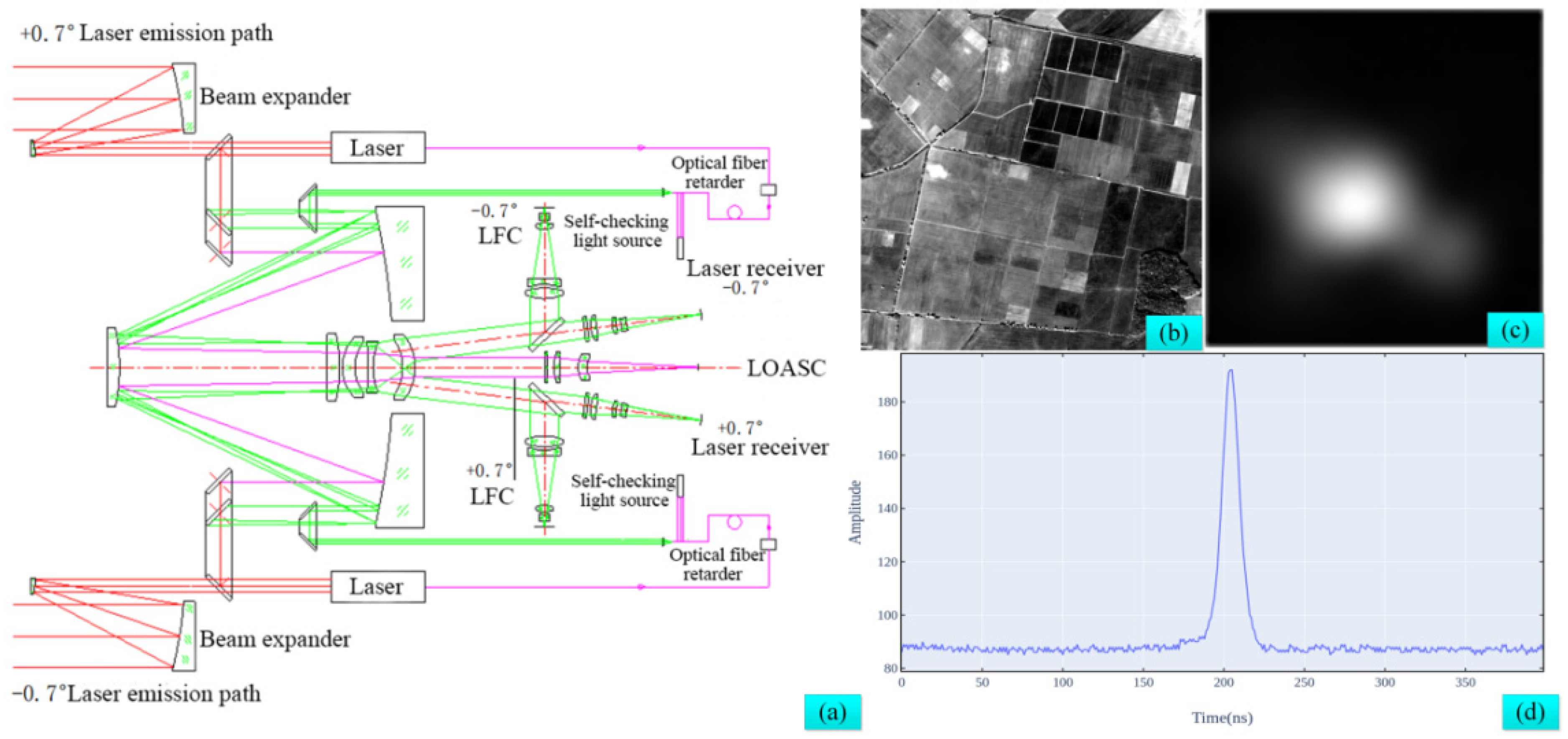
The GF-7 laser altimeter system is equipped with an LFC in addition to the laser altimeter. The LFC can acquire the laser footprint image (LFI) and laser center profile array (LCPA) (

Table 1. Comparison of laser footprint image (LFI) and laser center profile array (LCPA) parameters.

Project	LFI	LCPA
Image size	550 × 550 pixels	40 × 40 pixels
Operating spectral range	400–800 nm	1064 nm
Instantaneous field of view	0.19°	0.004°
Image type	panchromatic
Spatial resolution	3.2 m
Image quantization bit number	14 bits
Frequency of laser repetition	3 Hz
Laser emission energy	100–180 mJ

). As shown in Figure 1c and Table 1, when the laser reaches the receiving aperture of the LFC within 0.15 ms after laser emission, the LFC only images the laser spot. As shown in Figure 1b, either 15 ms before laser emission or 2 ms after laser spot imaging is completed, the LFC only images ground objects and obtains the LFI. The LFI’s main functions are as follows: (1) using the LFI to assist in evaluating whether the terrain in the area of the laser footprints is complex and whether it is affected by cloud cover [30]; and (2) based on the LCPA, analyzing the change in the laser spot centroid and directly exploring the change in the energy to determine the laser emissions state, which provides the basis for monitoring the laser pointing change and correcting the measurement error [18]. Figure 1a shows the internal optical path design of the GF-7 satellite laser altimetry system. Unlike ICESat/GLAS, which uses light from the laser spot with the full aperture through an optical mirror, the GF-7 satellite optical path uses light from the center of the spot captured by the LFC after quadruple beam expansion. Therefore, the detection result for the centroid change in the LCPA must be divided by four to obtain the change in the laser pointing angle corresponding to the emergent time of the laser beam, which corresponds to a change of approximately 0.31” for every offset pixel.

Figure 1d shows the laser emission waveform, which is the amplified waveform of the seed light inside the laser (corresponding to the “Laser” in Figure 1a) after numerous oscillations via the diode-pump array. Generally, there is almost no major change and it is in a stable state. However, at the emission time (corresponding to the “laser emission path” in Figure 1a), the laser beam may partially change, owing to interference from the satellite platform and other random factors, which further affect the positioning accuracy of the laser footprint.

2.2. Threshold Constrained for Extracting Centroid of the Ellipse-Fitting Method

For the LFIs, the facula and surrounding areas are affected by surface features. High-reflectivity features affect the results of traditional algorithms. In this study, we propose a threshold constraint for extracting the centroid with the ellipse-fitting method (TEFM), as shown in Figure 2, which can be divided into the following steps:

(1)

Remove the influence of background objects. Extract the slice of the LFI where the laser spot is located. Each pixel can be regarded as the superposition effect of the spot and ground object. After extensive statistical analysis, it was found that the histogram of the gray distribution in the background area tends to range from 2000 to 3000. The image is sliced to remove the influence of ground objects. We then subtracted 2000 from the overall gray value amplitude, as shown in Figure 2a.

(2)

Preliminary extraction of the laser spot contour based on the threshold method. Equation (1) was used to calculate the threshold value, T, and determine the initial extraction result of the light spot. As the first constraint, pixels smaller than the threshold value were assigned as 0. I(i,j) represents the gray value of the i^th row and j^th column in the image, and M and N represent the maximum and minimum values of the image rows and columns, respectively. Figure 3b shows the processing results, where some cloud areas are misidentified.

$$T=1/e^2\ast \max ({\displaystyle \sum _{i=1}^M{\displaystyle \sum _{j=1}^{N}I(i,j)-2000}}).$$

(1)

(3)

Morphological processing to remove noise. Morphological corrosion treatment method was employed on the results of Step 2. This aims to (a) remove the effect of fine noise, pores, and detailed texture features in the ground objects, (b) avoid the influence on subsequent steps, and (c) to a large extent, retain and approach the spot shape. As shown in Equation (2), the etching process extracts the local minimum in each pixel neighborhood (D1). I_src and I_dst, respectively, represent the spot image before and after processing. Figure 2c shows the processing results, where the etching treatment removed the pixels in the red-framed area.

$$I_{dst}(i,j)=\min {\displaystyle \sum _{i,j\in D_1}{I}_{src}(i,j)}.$$

(2)

(4)

Ellipse-fitting constrains the shape of the laser spot. We substituted the corrosion results into Equation (3), used least squares to fit the ellipse [16], and solved for the minimum value of the objective function, f, to determine each coefficient (A–F). The ellipse contour was used as the third constraint. The pixels outside the boundary were set as 0. The characteristic parameters of the light spots were retained, as shown in Figure 2d.

$$f(A,B,C,D,E)={\displaystyle \sum _{i=1}^M{\displaystyle \sum _{j=1}^N(A{i}^2+Bij+C{j}^2+Di+Ej+F}}{)}^2.$$

(3)

(5)

The GCM was used to extract the centroid of the laser spot, which is a classic algorithm for the centroid extraction of point light sources. This method yields different weights according to the gray distribution in the target area, followed by calculations of the centroid coordinates of the light spots. Even if the shape of the emitted laser spot is not strictly round or elliptical, better results can be achieved and the computational complexity remains low. However, directly using this method cannot avoid the influence of objects with high reflectivity in footprint images. Equations (4) and (5) provide the calculation methods, where (x,y) is the centroid coordinate of the laser spot:

$$x=\frac{{\displaystyle \sum _{i=1}^M{\displaystyle \sum _{j=1}^{N}i\ast I(i,j)}}}{{\displaystyle \sum _{i=1}^M{\displaystyle \sum _{j=1}^{N}I(i,j)}}} \mathrm{and}$$

(4)

$$y=\frac{{\displaystyle \sum _{i=1}^M{\displaystyle \sum _{j=1}^{N}j\ast I(i,j)}}}{{\displaystyle \sum _{i=1}^M{\displaystyle \sum _{j=1}^{N}I(i,j)}}}.$$

(5)

(6)

Removing gross errors based on spot-characteristic parameters. Ground object information on the LFI may cover the spot information, such that even the outline shape of the spot cannot be extracted, which could result in gross errors during processing. Therefore, according to the spot characteristics such as the eccentricity and long and short half axes, we must distinguish whether the spot information was successfully extracted to remove the errors. Based on our analysis, the ideal spot eccentricity was observed between 0.2 and 0.8, mainly due to light-emitting angle and the instrument’s internal frame. After the actual calibration, the laser spot diameter was between 17 and 20 m (beam at 1.19 and 2.21 m), corresponding to 5–7 pixels. However, to capture more information on the spot contour, this threshold was extended to the edge of the ideal divergent spot, whose value was 20.

Figure 3. Threshold constraint algorithm for extracting the centroid of the ellipse fitting. (a) LFI. (b) The result of laser spot contour extraction based on threshold method. (c) Morphological processing to remove noise. (d) Determine the centroid coordinates of laser spot by ellipse fitting method and GCM.

Figure 3. Threshold constraint algorithm for extracting the centroid of the ellipse fitting. (a) LFI. (b) The result of laser spot contour extraction based on threshold method. (c) Morphological processing to remove noise. (d) Determine the centroid coordinates of laser spot by ellipse fitting method and GCM.

2.3. Optical Transfer Function for Laser Emissions State Evaluation

The optical transfer function (OTF) is an index for evaluating the imaging quality of an optical system, which is defined as the ratio of the spatial frequencies of an object after imaging and transmittance through the optical system. Ideally, the frequency should not be lost, while the contrast should be 1. As previously discussed, directly applying the traditional OTF to the satellite on-orbit environment is difficult. Therefore, according to the characteristics of the GF-7 data, we proposed an optical transfer function for the laser emission state evaluation (OTF-LESE), which combines the emission waveform and LCPA. As is shown in Figure 4, the features of this function are as follows:

(1)

The laser emission state curve (f_TransWave^ith): slice around the laser spot while using the maximum radiance of each column to form a curve along the row direction, as shown in Equation (6), where I(x,y) represents the radiance of the x^th row and y^th column in the M × N LFI:

$$f_{TransWave}{}^{ith}=\max {\displaystyle \sum _{y=1}^{N}I(x_i,y)}(0\le i\le M).$$

(6)

(2)

Fourier transform: the spatial distribution features of the laser emissions waveform and laser emissions state curve are converted into frequency-domain features through a one-dimensional Fourier transform, as shown in Equation (7), where F(m) is the result of the Fourier transform at discrete points (e.g., k = 0, 1..., K − 1), m corresponds to the local frequency to be decomposed, X and f(x) correspond to the one-dimensional input data, and E^i2π represents the direction basis function of the transformation from the spatial domain to the frequency domain.

$$F(m)=\frac{1}{K}{\displaystyle \sum _{k=0}^{K-1}f(x)e^{i2\pi m\frac{k}{K}}}.$$

(7)

(3)

The modulation was calculated before and after transmission, as shown in Equation (8), which reflects the relative change in the spatial frequency at the current node, while F_max and F_min represent the maximum and minimum amplitude frequency after the Fourier transform, respectively:

$$C=\frac{F_{\max }-F_{\min }}{F_{\max }+F_{\min }}.$$

(8)

(4)

We constructed an optical transfer function for laser emissions state evaluation, as shown in Equation (9), where C_TransWave represents the modulation of the emission waveform and C_LaserSpot indicates the modulation of the laser spot:

$$OTF-LESE=\frac{C_{LaserSpot}}{C_{TransWave}}.$$

(9)

Figure 4. Calculation flow of the optical transfer function for laser emissions state evaluation. (a) Transmitted waveform of laser. (b) Fourier transform process. (d) Laser spot and its rendered image. (e) Laser emission state curve. (c,f) respectively correspond to Fourier change results of emission waveform and laser emission state curve.

Figure 4. Calculation flow of the optical transfer function for laser emissions state evaluation. (a) Transmitted waveform of laser. (b) Fourier transform process. (d) Laser spot and its rendered image. (e) Laser emission state curve. (c,f) respectively correspond to Fourier change results of emission waveform and laser emission state curve.

2.4. Other Evaluation Methods

2.4.1. Encircled Energy

Taking the centroid coordinates obtained by the TEFM as the center of the circle, the sum of the radiance within the statistical radius, R (in pixels), was referred to as the encircled energy graph, which can completely visualize the spot energy dispersion position. As listed in

Table 2. Multi-index evaluation of the laser-emitting state.

Indicator	Calculation Method
Encircled energy	$f(x_0,y_0,r)=Sum({\displaystyle \sum _{d=0}^{r}f(x,y)})$
Brightness of center disk	$f_{\max }=Max({\displaystyle \sum _{x=1}^M{\displaystyle \sum _{y=1}^{N}f(x,y))}}$ $f_{count}=Count({\displaystyle \sum _{x=1}^M{\displaystyle \sum _{y=1}^{N}f(x,y)(f\le 0.9f_{\max }))}}$

, the abscissa represents the radius, R, while the ordinate represents the total radiance in the containment circle (normalized). An increase in radius R produces a red circular area with more energy; the maximum slope of the encircled energy curve indicates the laser spot boundary.

2.4.2. Center Disk Brightness

When there were no interference factors in the optical system, the laser spot was a standard diffraction spot, which is annular, where the central bright spot accounted for approximately 90% of the energy and the first-order bright spot ring accounted for 10% of the energy. The encircled energy graph could only express the degree of energy dispersion, whereas the central lighting degree could express the amount of energy lost by the central bright spot. As listed in Table 2, the maximum brightness of the light spot and number of pixels was within 90% of the maximum brightness.

3. Results

3.1. Analysis of Long Time-Series Laser Pointing Change

To verify the accuracy and reliability of this method, the LFIs of the ascending orbit (at night) and complex ground objects were used as experimental data. As shown in Figure 5a, for night conditions, while avoiding a complex background, the centroid extraction accuracy of this method was within 0.05 pixels and the centroid extraction accuracy of the GCM was approximately 0.08 pixels. As shown in Figure 5b, under the influence of complex ground objects, the extraction accuracy of the centroid was within 0.08 pixels, which was approximately 2.5 pixels better than the result of the GCM. The error for the GCM mainly derived from exposure dispersion adjacent to the laser spot contour and the influence of background objects; this method removed these interference factors through multiple constraints. Under more complex background object conditions, the gap between the gray barycenter method and algorithm used in this study would be even greater.

To test the accuracy of the TEFM algorithm, 1600 LFIs with similar times and enriched ground object types were randomly selected for accuracy verification. Taking the calibration positions of the two beams in orbit as real values, the mean coordinate error, range, and root-mean-square error (RMSE) were calculated (

Table 3. Accuracy evaluation of centroid extraction algorithms for the footprint image.

Method a	Mean		Range		RMSE
	X	Y	X	Y	X	Y
GCM	2.565	2.522	4.941	5.185	2.512	2.218
TEFM	0.062	0.071	0.092	0.088	0.052	0.081

^a TEFM, the ellipse-fitting method; GCM, gray centroid method (GCM).

). The statistical results show that the traditional algorithm could not extract the centroid of the laser spots under a complex background. The TEFM algorithm maintained a high level of stability and overall extraction accuracy, which was one order of magnitude better than the traditional algorithm. Thus, the proposed algorithm conformed to the requirements of subpixel centroid extraction under complex background conditions.

From 15 to 30 March 2020, a total of 61 tracks of LFI data were extracted and 86,000 images were obtained. Among them, 27% of the images lost the spot contour information owing to cloud cover, overexposure, or other reasons, which made it impossible to extract the centroid. Figure 6 shows the experimental results. The abscissa represents the X-direction and the ordinate represents the Y-direction. The left side shows the statistical results for the centroid coordinates of beam #1, with mean coordinates of (120.83, 263.71). The X-direction oscillates at approximately 0.4 pixels, while the Y-direction oscillates at approximately 0.5 pixels. The plane position changes within 1 pixel. This is the statistical result for the centroid coordinates of beam #2 on the right side, with mean coordinates of (216.32, 162.51). The X-direction oscillates at approximately 0.5 pixels while the Y-direction oscillates at approximately 0.5 pixels. The plane position changes within 1 pixel. Therefore, we obtained the following preliminary conclusions: (1) compared with the traditional algorithm, the improved algorithm effectively extracts the centroid of the laser spot under a complex ground object background; and (2) the change in the centroid coordinates is relatively stable every month, in which the amplitude oscillation in the X- and Y-directions is <1 pixel.

The difficulty in establishing a long-term laser pointing monitoring system or extracting the centroid of a long time-series lies in eliminating gross errors and retaining the changing trend(s) of the centroid coordinates. Although many conditions can be used to constrain the spot contour and accurately locate the spot centroid position, the influence of background objects on the spot cannot be completely removed, which leads to gross errors, moves the coordinates of the spot centroid, and destroys the existing coordinate trend. There are two types of gross errors: (1) a high-reflectivity ground object completely covers the spot contour or (2) the amplitude of the laser spot itself is low and dim, such that the features of the light spot are hidden by the features of the ground objects. After a large number of statistical calculations, we found that the spot characteristic parameters, such as the eccentricity and half-axis length, could effectively identify gross errors and improve the overall recognition accuracy. To analyze the change and stability of the centroid of the footprint facula, analyses were carried out from both macroscopic and microscopic perspectives.

As listed in

Table 4. Statistical results of monthly mean of spot centroid coordinates of the laser footprint image (LFI; unit: pixel).

Time		LFI
		Laser #1		Laser #2
		X	Y	X	Y
2020	March	120.83	263.71	216.32	162.51
	April	120.50	264.51	216.88	162.63
	May	120.35	263.88	216.85	162.56
	June	120.37	263.79	216.87	162.36
	July	120.52	263.90	216.93	162.10
	August	120.63	263.28	216.81	161.65
	September	120.51	262.26	216.72	161.53
	October	120.11	261.85	216.35	161.60
	November	120.33	262.02	216.42	161.64
	December	120.37	262.30	216.31	161.82
2021	January	120.49	262.55	216.00	161.65
	February	120.36	262.55	216.81	161.17
	March	120.45	262.67	216.62	161.68
	April	120.43	262.63	216.63	161.07

, to perform long-term analyses on the stability of the spot centroid in the LFI since its orbital launch, the monthly mean coordinates of the facula centroid from March 2020 to April 2021 were counted. As shown in Figure 7a,b, for beam #1, the centroid coordinates showed a decreasing trend and changed by approximately 0.4 pixels in the X-direction and 1 pixel in the Y-direction. The plane position changed by approximately 1.1 pixels; the corresponding directional angle changed by approximately 0.341”. As shown in Figure 7c,d, for beam #2, the centroid coordinates first decreased and then increased by approximately 0.4 pixels in the X-direction. There was an overall decreasing trend in the Y-direction by approximately 1.5 pixels, a change in the plane position by approximately 1.4 pixels, and a change in the corresponding pointing angle by approximately 0.434”. For beams #1 and #2, the monthly change in the centroid of the spot did not always move in a specific direction; the monthly change had a relatively small range.

The laser footprint camera and the laser share the same receiving field of view. When the laser pointing jitter is small, the relative position of the laser footprint image and the laser spot is basically unchanged, and transmitting and receiving are coaxial, which can be regarded as the same reference coordinate system. In order to analyze the change in the plane accuracy of the laser data of the GF-7 satellite in orbit, this section randomly checks the plane accuracy of the long-time laser footprint image data. Google images, airborne aerial photographs (from Germany, China and other regions), and Lidar point clouds were used as reference data for evaluating the positioning accuracy of laser footprints [31,32]. As shown in

Table 5. Sampling inspection for plane accuracy evaluation of the laser footprint image (LFI; unit: pixel).

Time (Orbit Num)		LFI						Area
		Laser #1			Laser #2
		X *	Y *	RMS	X *	Y *	RMS
2020	March (002069)	−2.288	−3.636	4.771	−6.257	−1.419	7.177	China
	April (002662)	−2.973	−1.857	4.833	−2.287	0.333	4.490	China
	May (002814)	−0.830	0.300	2.219	−2.549	−1.649	3.893	China
	June (003516)	−0.152	−0.950	1.631	−0.979	0.033	2.368	Germany
	July (003723)	0.236	0.269	3.899	−0.367	1.053	2.638	China
	August (004331)	0.286	5.081	5.797	0.291	3.326	4.427	Google
	September (004817)	4.401	−4.131	7.209	−0.101	0.572	6.046	Google
	October (005382)	4.836	4.799	7.600	2.011	2.862	4.777	Google
	November (005729)	1.519	3.185	4.195	0.067	4.409	4.990	Google
	December (006432)	6.246	3.261	7.505	4.668	3.911	6.912	China

* represents the mean value of the coordinate offset in the X or Y direction.

, the positioning accuracy of lasers 1 and 2 is within two pixels, corresponding to a ground distance of ~6 m, which shows that the positioning accuracy of the laser footprint of the GF-7 satellite has remained relatively stable since its launch.

In the process of laser data processing and analysis of the GF-7 satellite, we found that the ranging and plane accuracy of the obtained laser spot is degraded to some extent when the satellite is rolling at a large angle; this may be related to: (1) the accuracy of the star sensor being reduced; (2) the angle of view of laser receiving becoming smaller; (3) pointing angle jitter at the time of emergent light; or (4) a change in the internal optical axis frame of the laser system due to temperature change, material thermal deformation, and other factors. We refer to the data obtained when the satellite rolling angle is greater than or equal to 3 as rolling data, as shown in

Table 6. Sampling inspection of plane accuracy evaluation of the laser footprint image (LFI) under the condition of the satellite in rolling (unit: pixel).

Time (Orbit Num)		LFI						Angle
		Laser #1			Laser #2
		X *	Y *	RMS	X *	Y *	RMS
2020	March (002706)	1.954	6.990	8.135	2.929	10.990	12.191	6.8
	April (002548)	7.770	0.002	8.338	9.674	1.623	10.353	7.3
	May (003057)	−6.420	−0.903	6.911	−9.138	−0.873	9.421	−10.5
	September (005608)	16.088	4.662	16.879	−19.550	3.711	22.084	9.6
	November (005593)	−1.345	3.059	3.852	−1.760	4.389	5.315	−4.6
	December (006186)	12.438	4.191	12.484	12.004	1.313	13.462	9.4

* represents the mean value of the coordinate offset in the X or Y direction.

, which is the random sampling result for evaluating the plane accuracy of rolling data. When the satellite swings sideways, the plane accuracy of beams 1 and 2 is ~two pixels or more, and the corresponding ground distance is 6–20 m. Compared with the case of no rolling, the plane accuracy of the footprint is greatly degraded, and the elevation value is uncertain. At present, the problem of laser ranging accuracy degradation caused by satellite pendulum measurement has not been solved, and the satellite rolling angle (3) can only be used as a necessary condition for quality control to control the overall accuracy. In this process, we found that satellite rolling has a certain influence on the distribution of laser spot energy (see Section 3.2).

3.2. Analysis of Long Time-Series Laser Energy Changes

To eliminate the influence of complex background objects on the radiance of the laser spot, we used nighttime data from April to July 2021 for the analysis. There were four tracks (one track sampled every month) and 6216 laser spots. Figure 8 shows the maximum amplitude of the center point, energy inclusion diagram, and OTF-LESE from top to bottom; beams #1 and #2 are shown from left to right. This analysis provided the following findings:

(1)

Brightness of center disk: As shown in Figure 8a,b, for beam #1, the maximum amplitude fluctuated between 5100 and 5600, with an amplitude jitter of 400 (dimensionless amplitude value) during the track crossing stage. The center energy gradually diffused after long-term operation. For beam #2, the maximum amplitude fluctuated between 2000 and 2600, with a jitter of 500 during the track crossing stage. The center energy was stable and tended to increase gradually during long-term operation.

(2)

Encircled energy diagram: As shown in Figure 8c,d, the maximum slope represented the spot boundary; the spot radius of beams #1 and #2 was between 8 and 10 pixels. With the centroid coordinate as the center and a radius within 20 pixels, the total energy of the scattered spot of beam #1 was approximately 1,200,000 (dimensionless amplitude value), while that of beam #2 was approximately 600,000 (approximately half that of beam #1). The amplitude value was not equal to the laser emission energy; there was a certain mapping relationship.

(3)

OTF-LESE: the maximum amplitude of the center point can only evaluate the change in the center value of the laser spot and the amount of energy lost, whereas the energy inclusion diagram can only show the energy dispersion degree adjacent to the spot but cannot fully evaluate the energy change at the time of light emission. As shown in Figure 8e,f, the range of the OTF-LESE was 0–1 under normal conditions; if it exceeded 1, the transmission waveform gain was too small. Compared with the first two indices, the OTF-LESE indicated that the periodic changes caused by the pointing jitter were considered during energy changes at the time of laser exit; there were notable periodic changes at the time of the crossing orbit for beams #1 and #2. For beam #1, the OTF-LESE changed within 0.7–1.3, with an average value of 0.91. The maximum amplitude changed to 0.3 when crossing the orbit, and the energy decayed to 0.7 with continuous operation. For beam #2, the OTF-LESE varied within 0.7–1.05, with an average value of 0.85. The maximum amplitude changed to 0.3 when crossing the orbit, and the energy decayed to 0.72 with continuous operation. This value was still within the normal working range for beams #1 and #2.

Figure 8. Analysis of changes in the laser energy at the emission time. (a,b) represent respectively center disk brightness of beam 1&2. (c,d) represent respectively Encircled energy diagram of beam 1&2. (e,f) represent respectively OTF-LESE of beam 1&2.

Figure 8. Analysis of changes in the laser energy at the emission time. (a,b) represent respectively center disk brightness of beam 1&2. (c,d) represent respectively Encircled energy diagram of beam 1&2. (e,f) represent respectively OTF-LESE of beam 1&2.

OTF-LESE is an index used to evaluate the output state of a satellite laser; using other values as the true values to verify its accuracy remains difficult. Here, we focused on evaluating the sensitivity and comprehensiveness to various changes in the laser state. As shown in Figure 9 and

Table 7. Screening indicators for land area data.

Index	1258625622	1258623582	1258623914	1262783002
OTF-LESE a	0.7	0.8	0.9	1.0
Kurtosis	−2.52	−2.32	−2.03	−1.86
Skewness	0.66	0.67	0.72	0.73
Waveform Width/ns	5.68	5.62	5.55	5.45

^a Optical transfer function (OTF)-laser emission state evaluation (LESE).

, from left to right, the OTF-LESE was 0.7, 0.8, 0.9, and 1.0. The upper sequence diagram shows the transmission waveform while the lower sequence diagram shows the LCPA data. When the satellite laser was launched, the peak and amplitude of the emission waveform, coordinates for the centroid of the spot in the LCPA, and energy distribution, were in a relatively stable state within a small range. Taking the laser state of the rightmost OTF-LESE as a reference, the plane coordinate for the center of mass of the leftmost laser LCPA changed by approximately 0.8 pixels, the spot radius decreased by approximately 1.2 pixels (with 80% of the central energy amplitude as the constraint based on the energy inclusion diagram), and the central energy amplitude decreased by approximately 80. The peak value of the leftmost emission waveform decreased by approximately 10, the kurtosis coefficient changed by approximately 0.66, the skewness coefficient changed by approximately 0.07, and the waveform width decreased by approximately 0.23. Based on these parameters, the OTF-LESE can represent the typical characteristics of the output state of the satellite laser.

On 3 December 2020, the GF-7 satellite passed over Lake Tanganyika at night, acquiring 18 laser spots, including 10 points from beam #1 and 8 points from beam #2 (Figure 10). Combined with meteorological data, it is confirmed that there were no waves on the lake when the data were obtained, which would not cause additional observation error. Tanganyika is a freshwater lake in central Africa, with a coastline of 1900 km. Considering the influence from the curvature of Earth, the elevation of the lake presents a linear trend along the track. Therefore, the height profile data for beams #1 and #2 along the rail direction were fitted separately. The height error of the corresponding position was calculated as the true value. The maximum error of beam #1 was 7 cm and that of the OTF-LESE was 0.68. The maximum error of beam #2 was 14 cm and that of the OTF-LESE was 0.63. Regardless of the stability of the working mode or altimetry accuracy, beam #1 was superior to #2.

To further verify whether the OTF-LESE could effectively estimate the emission state of the satellite laser and further estimate the altimetry error caused by the change state, we analyzed the correlation between the altimetry error and OTF-LESE of the data on the lake, collected using the two beams. As shown in Figure 11, the OTF-LESE had a positive correlation with the altimetry error caused by the jitter of the laser state. The Pearson correlation coefficient between the two variables was 0.78, which shows that the OTF-LESE effectively evaluated the emission state of the satellite laser and provided data quality control for the final altimetry product.

4. Discussion

In this manuscript, based on the LFIs, we propose a method for evaluating the launch state of satellite laser altimeter, which mainly includes two parts: laser pointing change monitoring and energy distribution monitoring. Based on these methods, we analyze and evaluate the actual data of the GF-7 satellite. Before the GF-7 satellite, there was no laser altimetry system equipped with LFC. Therefore, it is of great significance to evaluate the launching state of the manuscript based on LFIs.

For the satellite laser altimetry system, the external environment has a great influence on the measurement accuracy of the plane and elevation of laser footprints [33]. Yao et al. found that the multiple scattering effect caused by cloud has a significant influence on the ranging accuracy of GF-7 data [15,34], but in addition, when the area covered by cloud coincides with the area where the light spot is located, it will affect the original internal characteristics, thus affecting the laser pointing and energy distribution monitoring accuracy. In addition to clouds, glaciers, deserts and other highly reflective features will also have the same impact. In Section 3 of the manuscript, because the laser spot on LFI acquired in daytime may be affected by ground objects and clouds, the data acquired by the GF-7 satellite at night are used as experimental data to avoid the influence of potential errors. It can be seen from Figure 1a that LFI is an image formed by acquiring laser spots and background objects from two light paths, so the background objects that acquire data at night will not affect the evaluation of laser-emission state. In order to analyze the change in footprint plane accuracy caused by laser pointing jitter, Google images and aerial photographs are introduced as reference data for accuracy evaluation, and their plane accuracy is ~1 m [31,32]. During the data processing of the GF-7 satellite, we found that the laser pointing changed little every month, so we randomly selected one track from the night data obtained every month as experimental data to analyze the plane accuracy of laser footprints in long time series. The experimental results show that the laser pointing jitter is about 0.3″, and the corresponding laser footprint positioning accuracy is about 5 m. Compared with complex surface, ideally, the accuracy of satellite laser altimetry in water should have higher internal consistency, but meteorological factors such as wind speed may introduce additional observation errors [34]. According to the monthly meteorological data provided by NOAA’s National Centers for Environmental Information (NCEI) during data collection [35], we found that the wind speed was less than 3 m/s, which would not cause waves on the lake. After excluding the influence of external environmental factors, we can confirm that these altimetry errors may be caused by the change in laser emission state, which is also proved by the high correlation between them.

Sirota et al. [19] found that the ICESat spot center-of-mass coordinates show a periodic variation, which corresponds to the long arc period of the satellite’s motion with respect to the star. This pattern of variation was not found in the GF-7 data for the following reasons: (1) ICESat spot images can acquire the complete cross-section of the laser pulse, while the GF-7 satellite is designed to adopt a different imaging mode, with its spot images acquiring only the central region of the pulse cross-section and directing light to the laser footprint camera; (2) compared with ICESat, the GF-7 satellite has a greater improvement in thermal control technology, which can weaken the influence of stellar radiation. During the processing of the GF-7 laser data, it was found that as the laser continued to operate, the laser center-of-mass shift would increase and OTF-LESE would decrease, which was caused by some deformation of the optical axis frame inside the instrument due to temperature changes. Although this effect is small, it is still worth focusing on and continuing to optimize in subsequent research work.

5. Conclusions

Based on the LFC of the GF-7 satellite, this study evaluated the launch state of the satellite laser altimeter. We obtained the following conclusions:

• Compared with the traditional centroid extraction algorithm, the improved algorithm proposed in this study accurately extracted the centroid coordinates of the laser footprint images in complex ground objects. The centroid extraction accuracy was within 0.08 pixels, which is approximately 2.5 pixels better than that of the GCM.
• In the laser footprint image, the plane position of beam #1 changed by approximately 1.1 pixels; the corresponding change in the pointing angle was approximately 0.341″. The change in the position of ~6 m. When the satellite rolling angle is greater than 3, the positioning accuracy of the laser footprint is ~6–20 m. Satellite rolling measurement has a significant influence on the positioning and ranging accuracy of laser footprints, but the existing theoretical model cannot be completely revised; this requires further discussion.
• Compared with the central brightness and encircled energy diagram, the OTF-LESE considered the image of the laser state, energy distribution, and other factors, which were more suitable for evaluating the satellite laser exit state.
• When the laser operated continuously, the internal energy transfer efficiency of the system decreased gradually. The corresponding OTF-LESE decreased from 1 to 0.7. The experimental results show that this index effectively evaluates the laser emissions state of the satellite.

References

- Li, G.; Guo, J.; Pei, L.; Zhang, S.; Tang, X.; Yao, J. Extraction and analysis of the 3-D features of crevasses in the Amery Ice Shelf based on ICESat-2 ATL06 data. IEEE J. Sel. Top. Appl. Earth Obs. Remote Sens. 2021, 99, 1–12. [Google Scholar] [CrossRef]
- Yao, J.; Gao, X.; Li, G.; Yang, X.; Lu, J.; Li, C. Cloud optical depth inversion of echo energy data based on ICESat/GLAS. Infrared Laser Eng. 2019, 48, 126–134. [Google Scholar]
- Yao, J.; Tang, X.; Li, G.; Ai, B.; Yang, X.; Xie, D. Cloud Detection of Laser Altimetry Satellite ICESat-2 and the Related Algorithm. Laser Optoelectron. Prog. 2020, 57, 248–256. [Google Scholar]
- Xie, D.; Li, G.; Zhao, Y.; Yang, X.; Yang, X.; Fu, A. GEDI Space-based Laser Altimetry System and its Application. Space Int. 2018, 12, 39–44. [Google Scholar]
- Yang, X.; Li, G.; Wang, P.; Chang, X.; Yao, J. Monitoring of Qing hai Lake changes with spaceborne laser altimetry and remote sensing images. Sci. Surv. Mapp. 2020, 45, 83–91. [Google Scholar]
- Wang, X.; Cheng, X.; Gong, P.; Huang, H.; Zhan, L.; Xiaowen, L. Earth science applications of ICESat/GLAS: A review. Int. J. Remote Sens. 2011, 32, 8837–8864. [Google Scholar] [CrossRef]
- Abdalati, W.; Zwally, H.J.; Bindschadler, R.; Csatho, B.; Farrell, S.L.; Fricker, H.A.; Harding, D.; Kwok, R.; Lefsky, M.; Markus, T. The ICESat-2 Laser Altimetry Mission. Proc. IEEE 2010, 98, 735–751. [Google Scholar] [CrossRef]
- Michelle, H.S.S.; Yi, D. Algorithm Theoretical Basis Document for GEDI Transmit and Receive Waveform Processing for L1 and L2 Products (Goddard Space Flight Center, 2019). Available online: https://gedi.umd.edu/ (accessed on 23 December 2021).
- Li, G.; Tang, X. Analysis and Validation of ZY-302 Satellite Laser Altimetry Data. Acta Geod. Cartogr. Sin. 2017, 46, 1939–1949. [Google Scholar]
- Li, G.; Gao, X.; Chen, J.; Zhao, Y.; Mo, F.; Zhang, Y. Data quality analysis of ZY-3 02 satellite laser altimeter. J. Remote Sens. 2019, 23, 1159–1166. [Google Scholar]
- Tang, X.; Xie, J.; Liu, R.; Huang, G.; Dou, X. Overview of the GF-7 Laser Altimeter System Mission. Earth Space Sci. 2019, 7, e2019EA000777. [Google Scholar] [CrossRef]
- Meng, J.; Zhang, X.; Jiang, J.; Wu, Y.; Xie, K.; Wei, S.; Wang, J.; Wang, Z.; Chen, W. Design of Laser Transmitter for GF-7 Satellite Laser Altimeter. Spacecr. Eng. 2020, 29, 96–102. [Google Scholar]
- Cao, H.; Zhang, X.; Zhao, C.; Xu, C.; Mo, F.; Dai, J. System design and key technologies of the GF-7 satellite. Chin. Space Sci. Technol. 2020, 40, 1–9. [Google Scholar]
- Li, G.; Tang, X.; Chen, J.; Yao, J.; Liu, Z.; Gao, X.; Zuo, Z.; Zhou, X. Processing and preliminary accuracy validation of the GF-7 satellite laser altimetry data. Acta Geod. Cartogr. Sin. 2021, 50, 1338–1348. [Google Scholar]
- Tang, X.; Yao, J.; Li, G.; Ai, B.; Gao, X. Influence of cloud scattering on satellite laser altimetry data and its correction. Appl. Opt. 2020, 59, 4064–4075. [Google Scholar] [CrossRef]
- Fan, C.; Li, J.; Wang, D.; Zhang, Y.; Shi, X. ICESAT/GLAS laser footprint geolocation and error analysis. J. Geod. Geodyn. 2007, 27, 104–106. [Google Scholar]
- Liu, Z.; Huang, G.; Liao, Y.; Xie, F. Preliminary study on laser spot characteristics of GF-7 laser altimeter. Informatiz. China Constr. 2020, 120, 82–83. [Google Scholar]
- Yao, J.; Li, G.; Chen, J.; Zhou, X.; Guo, A.; Huang, G.; Tang, X.; Ai, B. Analysis on the change of GF-7 satellite laser altimeter on-orbit spot centroid position. Infrared Laser Eng. 2021, 50, 20210539. [Google Scholar]
- Sirota, J.M.; Bae, S.; Millar, P.; Mostofi, D.; Webb, C.; Schutz, B.; Luthcke, S. The transmitter pointing determination in the Geoscience Laser Altimeter System. Geophys. Res. Lett. 2005, 32, 1–18. [Google Scholar] [CrossRef]
- Waerbeke, L.V.; Mellier, Y.; Erben, T.; Cuillandre, J.C.; Schneider, P. Detection of correlated galaxy ellipticities on CFHT data: First evidence for gravitational lensing by large-scale structures. Astron. Astrophys. 2000, 358, 1–12. [Google Scholar]
- Bae, S.; Webb, C.; Schutz, B. GLAS PAD Calibration Using Laser Reference Sensor Data. In Proceedings of the AIAA/AAS Astrodynamics Specialist Conference and Exhibit, Providence, RI, USA, 16–19 August 2004. [Google Scholar]
- Yuan, X.; Li, G.; Tang, X.; Gao, X.; Huang, G.; Li, Y. Centroid Automatic Extraction of Spaceborne Laser Spot Image. Acta Geod. Cartogr. Sin. 2018, 47, 135–141. [Google Scholar]
- Yang, X.; Li, G.; Wang, P.; Chen, J.; Mo, F.; Yao, J.; Jin, Z. Laser pointing changes detection method for space-borne laser spot image. Acta Geod. Cartogr. Sin. 2020, 49, 86–94. [Google Scholar]
- Yang, X.; Li, G.; Yao, J. Laser pointing and characterization parameter determination methods based on laser profile arrays of ICESat/GALS. Opt. Express 2021, 29, 9861–9877. [Google Scholar] [CrossRef] [PubMed]
- Feltz, J.C.; Karim, M.A. Modulation transfer function of charge-coupled devices. Appl. Opt. 1990, 29, 717–722. [Google Scholar] [CrossRef]
- Zhang, M. Evaluation Method of CCD Camera Imaging Quality Based on MTF. Master’s Thesis, Changchun University of Science and Technology, Changchun, China, 2015. [Google Scholar]
- Zhang, W. Evaluation of Light Cone Imaging Quality by MTF. Master’s Thesis, Graduate School of Chinese Academy of Sciences, Xi’an, China, 2006. [Google Scholar]
- Li, Y. Encircled energy for systems of different Fresnel numbers. Energy Proc. 1983, 64, 207–218. [Google Scholar]
- Stamnes, J.J.; Heier, H.; Ljunggren, S. Encircled energy for systems with centrally obscured circular pupils. Appl. Opt. 1982, 21, 1628–1633. [Google Scholar] [CrossRef] [PubMed]
- Yao, J.; Tang, X.; Li, G.; Guo, J.; Ai, B. Cloud detection of GF-7 satellite laser footprint image. IET Image Process 2021, 15, 2127–2134. [Google Scholar] [CrossRef]
- Land NRW. Digitales Geländemodell Mittlerer Punktabstand 1m-dl-de/by-2-0. 2019. Available online: http://www.govdata.de/dl-de/by-2-0 (accessed on 11 August 2021).
- Ragheb, A.E.; Ragab, A.F. Enhancement of Google Earth Positional Accuracy. Int. J. Eng. Res. Technol. 2015, 4, 627–630. [Google Scholar]
- Zhang, Z.; Xie, H.; Tong, X.; Zhang, H.; Li, B. Research progress of full waveform processing technology of satellite laser altimetry. Sci. Surv. Mapp. 2019, 44, 168–178. [Google Scholar]
- Yao, J.; Tang, X.; Li, G.; Chen, J.; Zuo, Z.; Ai, B.; Zhang, S.; Guo, J. Influence of Atmospheric Scattering on the Accuracy of Laser Altimetry of the GF-7 Satellite and Corrections. Remote Sens. 2022, 14, 129. [Google Scholar] [CrossRef]
- Smith, A. NOAA NCEI, 2018: U.S. Billion-Dollar Weather and Climate Disasters, NOAA National Centers for Environmental Information (NCEI). 2018. Available online: https://www.ncdc.noaa.gov/billions (accessed on 11 August 2021).
Figure 1.
(a) Optical path of the laser system. (b) Laser footprint image. (c) Laser center profile array. (d) Laser emissions waveform.
Figure 2.
Flowchart of the ellipse-fitting method (TEFM) algorithm.
Figure 5.
Accuracy evaluation of the proposed algorithm. Red, blue, and yellow dots correspond to the centroid calibration position, (a) the centroid extraction result of the ellipse-fitting method (TEFM), and (b) the centroid extraction result of the gray centroid method (GCM), respectively.
Figure 6.
Centroid coordinate statistics for the laser footprint image (LFI) of laser 1 (a) and 2 (b).
Figure 7.
Changes in the centroid of the two beams in the X- and Y-directions on the laser footprint image (LFI). (a,b) respectively correspond to the monthly changes of the coordinates of the centroid of the laser spot of laser1 in the X and Y directions. (c,d) respectively correspond to the monthly changes of the coordinates of the centroid of the laser spot of laser2 in the X and Y directions.
Figure 9.
Several typical cases of the optical transfer function (OTF)-laser emission state evaluation (LESE). (a–d) Transmission waveform. (e–h) LCPA.
Figure 10.
(a) Distribution of laser spots across Lake Tanganyika. (b) Height profile of beam #1 along the track and (c) height profile of beam #2 along the track.
Figure 11.
Correlation analysis between the optical transfer function (OTF)-laser emission state evaluation (LESE) and altimetry error.