
Time-Range Adaptive Focusing Method Based on APC and Iterative Adaptive Radon-Fourier Transform

1
Marine Target Detection Research Group, Naval Aviation University, Yantai 264001, China
2
92337 Troop, PLA, Dalian 116000, China
*
Author to whom correspondence should be addressed.
Remote Sens. 2022, 14(23), 6182; https://doi.org/10.3390/rs14236182
Submission received: 28 July 2022
/
Revised: 15 September 2022
/
Accepted: 23 September 2022
/
Published: 6 December 2022
(This article belongs to the Special Issue Radar High-Speed Target Detection, Tracking, Imaging and Recognition)
Abstract
:In conventional radar signal processing, the cascade of pulse compression (i.e., matched filter) and Radon-Fourier transform (RFT) can extract the estimated scattering coefficient of the target in the range-velocity dimension through long-time coherent integration (i.e., long-time focusing). However, matched filter has problems such as range sidelobes. RFT belongs to a standard time-dimension matched filter, which will cause velocity sidelobes of strong targets. The range-velocity sidelobes caused by matched filter and RFT will mask other weak targets and affect the subsequent signal processing processes such as target detection and tracking. To suppress range-velocity sidelobes and achieve better range-velocity focusing, this paper proposes a time-range adaptive focusing method named APC-IARFT for short, which is based on adaptive pulse compression (APC) and newly proposed iterative adaptive Radon-Fourier transform (IARFT). In the APC-IARFT method, the radar time-range adaptive focusing consists of two steps: range-dimension adaptive focusing and long-time adaptive focusing in the velocity dimension. The APC method can realize range-dimension adaptive focusing and suppress range sidelobes of strong targets. Then, based on the minimum variance distortionless response (MVDR) formulation, the proposed IARFT method iteratively designs time-dimension adaptive filter of each range-velocity grid according to the received signal processed by APC to suppress velocity sidelobes of strong targets and achieve long-time adaptive focusing. Compared with the conventional cascade of matched filter and RFT, the cascade of matched filter and adaptive Radon-Fourier transform (ARFT), the results show that the proposed time-range adaptive focusing method (i.e., APC-IARFT) is competent for a variety of scenarios.
1. Introduction
In the conventional radar signal processing, the cascade of matched filter and moving target detection (MTD) method has been widely applied by modern coherent radar. As the conventional coherent integration method, the MTD method implies the assumption that the target is only in one single range cell during the coherent processing interval (CPI). For high-speed weak targets like unmanned aerial vehicles, due to their low signal-to-noise ratios (SNRs), increasing CPI helps improve the SNRs of high-speed weak targets, but the targets will cross multiple range cells during the CPI. At the same time, modern high-resolution radar aggravates the targets’ across range cells (ARC) problem due to the targets’ velocities, so the conventional coherent integration method is facing serious performance degradation.
To solve these problems, various long-time coherent integration (i.e., long-time focusing) methods have been proposed to form a cascade with matched filter and implement time-range two-dimensional focusing, such as the long-time coherent integration method based on Keystone transform [1,2,3,4], three-dimensional matched filter [5], etc. In these early methods, the processing flows are complex, and most of the methods correct range migration and realize coherent integration in sequence. For linear moving targets, Professor Jia Xu systematically proposed a long-time focusing method based on Radon-Fourier transform [6,7,8] for the first time, which solves the ARC problems of moving targets. RFT can be regarded as a generalized Doppler filter. As a generalized form of RFT, generalized RFT (GRFT) can be used for focusing of various motion styles theoretically [6,9]. It is known that the two drawbacks of RFT are blind-speed sidelobes (BSSL) and the computational cost of the search of two-dimensional parameters [7,8]. For the first drawback, improving the range resolution, increasing the number of coherent pulses, and weighting the Doppler filter of RFT are beneficial to suppress BSSL [7]. For the second drawback, fast implementation methods based on fast Fourier transform and particle swarm optimization algorithm are proposed respectively [8,10]. Afterward, the RFT method is further extended to wideband radar field and array signal processing [11,12]. Professor Xu further proposed the idea of Space-Time-Frequency Focus-Before-Detection (STF-FBD) on the basis of RFT theory [13], which utilizes multi-dimensional coherent integration to achieve the optimal energy focusing, target detection, parameter estimation, maneuver tracking, feature extraction and target recognition. Through the joint processing of space (i.e., array), velocity (i.e., pulse) and range (i.e., waveform), the focusing of target’s energy in multi-dimensional space is achieved, which laid a theoretical and technical foundation for improving radar target detection in complex environment. To reduce the computational cost of long-time focusing, Jia Xu divides the long CPI into several sub-apertures, and utilizes moving target detection (MTD) for coherent integration in every sub-aperture, then utilizes non-coherent integration between sub-apertures [14]. However, the method in [14] only considers a single high-speed maneuvering target, without considering the impact of multiple targets. Jia Xu’s team further combs the challenges and the latest research progress of long-time focusing methods related to Focus-Before-Detection (FBD) [15,16]. It can be seen that relevant research based on FBD theory continue to emerge and FBD has become a hot research field in recent years. Xiaolong Chen et al. consider the Doppler spectrum broadening caused by acceleration, and propose a Radon-Fractional Fourier transform (RFRFT) method for the detection of maneuvering targets [17] and a kind of Radon-Linear canonical transform method for the detection of targets with micromotion in sea clutter [18].
Because the RFT method is aimed at high-speed moving targets, the searching interval of velocity used in the RFT method usually exceeds the range of maximum unambiguous velocity in the MTD method. Since RFT can be regarded as the expansion of Fourier transform, it will cause velocity sidelobes masking other weak targets. In addition, RFT is not an adaptive processing method. Xu and Yan extend the RFT to the adaptive clutter suppression [19], and then propose sub-aperture adaptive RFT (SA-ARFT) method to relax the requirements for the amount of independent and identically distributed data and reduce the computational cost. However, the adaptive method in [19] is aimed at clutter suppression, and does not have the ability of adaptive suppression for the jamming targets in the training samples. Pengjie You et al. also consider the adaptive GRFT in clutter background, and derive the Cramer-Rao lower bound of parameter estimation [20]. Its essence is same as that in [19], so it is also limited by the independent and identically distributed training samples, and does not have the ability to adaptively suppress jamming targets. Zegang Ding utilizes adaptive RFT (ARFT) method after dividing the parameter space into subspaces, and balances the computational cost and detection performance by adjusting the length of every subspace [21]. The ARFT method uses the inverse of clutter covariance matrix to form clutter notch and suppress clutter, which is helpful to focus the target energy in a clutter background. However, when the target’s velocity is too high, which causes the fluctuation of amplitude between pulses and makes the number of effective pulses available for long-time focusing is limited, the velocity resolution of the ARFT method will decrease, and the performance of focusing will degrade.
On the other hand, the mathematical model of Doppler estimation is similar to that of direction of arrival (DOA) estimation, so the research related to DOA estimation can also be used to solve the problems of Doppler (velocity) sidelobes suppression and velocity resolution. Conventional DOA estimation methods such as MUSIC [22], root-MUSIC [23] and ESPRIT [24] use the spatial snapshots to calculate the sample covariance matrix (SCM) to estimate the unknown spatial covariance matrix, and use SCM to estimate the number and direction of signal sources. Professor Blunt proposes a reiterative super-resolution (RISR) method, which was originally used for DOA estimation in array signal processing [25,26]. The RISR method is based on the minimum mean square error (MMSE) criterion. The method does not need the prior knowledge of the number of signal sources, and can automatically determine the number, direction, and power of signal sources. Given the information about the spatial covariance of noise and one snapshot, the RISR method iteratively updates the structured MMSE filter bank by using the previous estimation of spatial power distribution, and applies the filter bank to the echo signal to update the estimation of spatial power distribution. Based on the same theoretical basis, Professor Blunt applies the RISR method to time dimension to get high-resolution frequency estimation [26], proposes adaptive pulse compression (APC) method in the range dimension [27], and proposes space-time adaptive processing [28], time-range adaptive processing [29], which are adaptive methods combining different dimensions. Almost at the same time, Professor Jian Li proposed a nonparametric iterative adaptive approach (IAA) [30]. The IAA method comprehensively considers the range-Doppler two-dimensional joint estimation, and its essential idea is the same as that of the APC method [31]. Although the IAA method iterates over the whole echo data and has a large amount of computational cost, it does effectively improve the resolution and estimation accuracy in active sensing such as range-Doppler imaging and passive sensing such as underwater acoustic measurements.
From the above analysis, it can be seen that the idea of iterative adaptive processing in the RISR method (or APC method) and IAA method has the ability of sidelobes suppression, and the ability is conducive to energy focusing. However, the existing relevant methods of IAA also imply the assumption that the target is only located in one range cell within the CPI, and the IAA method considering the ARC problem has not been put forward. In order to solve the sidelobes masking problem in range-velocity domain, this paper proposes a time-range adaptive focusing method (which is named APC-IARFT for short) based on APC and iterative adaptive Radon-Fourier transform (IARFT). Based on the concept of focusing proposed by Jia Xu [15,16], this method first utilizes the APC method to realize the adaptive focusing in range dimension and suppress range sidelobes of strong targets, then uses the IARFT method which is first proposed in this paper to realize the long-time adaptive focusing and suppress velocity sidelobes. The IARFT method draws on the idea of iterative adaptive processing mentioned in both the RISR method and IAA method. This method is based on the minimum variance distortionless response (MVDR) criterion [32], and an adaptive filter is estimated for the echo signal of each range-velocity grid in the method [33]. Through the cascade of APC method and IARFT method, APC-IARFT method adaptively suppresses range-velocity sidelobes of strong targets in the range-velocity two-dimensional output, so as to achieve better focusing and accurately obtain the range and velocity information of weak targets.
APC-IARFT method consists of range-dimension adaptive focusing and velocity-dimension adaptive focusing, so the content of this paper is organized as follows. In Section 2, the signal model of pulse trains is constructed. In Section 3, the APC method is utilized in range dimension to achieve range-dimension adaptive focusing and obtain the data of pulse trains processed by APC. In Section 4, IARFT method is utilized to process the data obtained by APC, so as to obtain the final output of the APC-IARFT method. In Section 5, we discuss the termination conditions of the iteration and computational cost about IARFT method. Finally, the performance of the APC-IARFT method is verified by experiments in Section 6.
2. Signal Model
Suppose that the waveform of the pulse transmitted in the radar system is recorded as vector s. There are N points in the pulse, , is pulse width, is sampling frequency. and is represented as
where is the sampling interval, 0 ≤ n ≤ N − 1, and rect(·) is the rectangular window. modulation(·) is the modulation form of pulse signal, which can be linear frequency modulation, nonlinear frequency modulation or other complex modulation forms. This paper is mainly based on linear frequency modulation. When a high-speed target moves across range cells within CPI T, its trajectory is recorded as r(t) [6].
where t is the time variable in [−T/2, T/2]. is the position of the target at time 0, and is the radial velocity of the target. Since the high-speed movement of the target will affect the amplitude and phase of its radar cross section, the size of T is limited in order to ensure that the target energy can be coherently integrated. Suppose the high-order motion of the target [34,35] in the limited CPI T is not obvious, so remains unchanged.
After down conversion and analog-to-digital conversion, the radar received echo data matrix Y of coherent pulse trains in CPI T can be expressed as Y = X + N. X is the matrix composed of targets’ echo signal, and N is the matrix composed of noise, clutter, and jamming. Set pulse repetition interval (PRI) as TPRI, Np = T/TPRI is the number of coherent pulses. There are D range cells in the scene, therefore Y is a Np × D-dimensional matrix composed of Np row vectors, representing the echo data of Np PRIs within T. It is assumed that the echo vector signal y(m,d) (y(m,d) Y) of the d-th range cell (1 ≤ d ≤ D) in the m-th PRI (1 ≤ m ≤ Np) before conventional pulse compression (i.e., matched filter) can be expressed as
where x(m,d) = [ x(m,d), x(m,d−1),…, x(m,d−N+1)]T represents the N-point continuous sampling of the real scene in the m-th PRI and x(m,d) is the real scattering coefficient of the d-th range cell in the m-th PRI. n(m,d) is the additive Gaussian white noise at the d-th range cell in the m-th PRI and (·)T is the transpose operation.
Suppose YPC is the data matrix of the coherent pulse trains processed by conventional pulse compression (i.e., matched filter), and the echo vector signal ( YPC) of the d-th range cell in the m-th PRI after matched filter can be expressed as
where y(m,d) = [y(m,d), y(m,d+1), …, y(m,d+N−1)]T is the N-point continuous sampling of the echo pulse corresponding to the d-th range cell in the m-th PRI and , . is the noise vector and (·)H is the conjugate transpose operation.
3. Range-Dimension Adaptive Focusing Based on Adaptive Pulse Compression
The results of matched filter are often affected by the autocorrelation and cross-correlation of the transmitted signals. The weak target is easy to be covered by strong targets’ range sidelobes, and the resolution of matched filter is limited. In order to achieve better range-dimension pulse compression and energy focusing, the adaptive filter designed in APC method for y(m,d) is expressed as follows
where ( YAPC) is the echo data of the d-th range cell in the m-th PRI processed by APC method and YAPC is the data matrix of the coherent pulse trains processed by APC method. is the weight vector of APC method which corresponds to the d-th range cell in the m-th PRI. Based on MVDR criterion, the cost function of weight vector is as follows [27,32],
where is the cost function of APC method which corresponds to the d-th range cell in the m-th PRI. is the real scattering coefficient of the d-th range cell in the m-th PRI, and E[·] is the expectation operator. According to Equation (6), the Lagrange multiplier method is used to minimize [36]. Assuming that the scattering coefficient remains unchanged in T, the coefficients in different range cells are not correlated with each other, and are not correlated with noise. The expression of can be obtained as
where is the echo covariance matrix, and is the covariance matrix of noise, which can be simplified as ( is the power of noise). is the signal covariance matrix [37],
where is the power estimation of the (d + p)-th range cell in the m-th PRI, −N + 1 ≤ p ≤ N − 1 [27,38]. contains the elements of the waveform s shifted by p samples,
Repeat the above process for the range-dimension echo signal received in all PRIs to obtain data YAPC of the coherent pulse trains, then the range-dimension pulse compression and adaptive focusing are completed. So YAPC obtained by APC method can be viewed as the ideal input for the IARFT method.
4. Long-Time Adaptive Focusing Based on Iterative Adaptive Radon-Fourier Transform
The idea of iterative adaptive processing in the IARFT method derives from the idea of IAA, which is originally used for signal source localization in array signal processing [30]. At present, IAA has been extended to Doppler-dimension processing, range-dimension processing, and other fields such as multi-dimensional signal processing. As a nonparametric method derived based on the weighted least squares criterion [30], IAA aims to solve the estimation problem of coefficients in the following linear models [39]:
where is the steering vector and is the noise vector. So as to realize IARFT method, we need to build a linear model which is in the same form as Equation (10) based on data YAPC in Section 3. This linear model needs to be related to the two parameters: range and velocity. In this section, we need to first discretize the parameter space of range and velocity into two-dimensional grids, and then use the two-dimensional grids to establish the linear model like Equation (10). Only in this way can the filter of the IARFT method be deduced according to the linear model.
4.1. Setting of Range-Velocity Grid in IARFT Method
The long-time adaptive focusing method based on IARFT method searches the range cells that high-speed target passes through in CPI T to focus the target’s energy. Generally, the data YAPC contains two parts: one part is the search area which we are interested in, and the other part is the data extraction area. The data extraction area includes the search area. Figure 1 shows the relationship of the search area and the data extraction area in YAPC. Set the center of the search area as rC, and ra stands for the range of search area. The initial position at time 0 and velocity of the target are unknown, so it is necessary to search the parameters in the searching interval of range [rC − ra/2, rC + ra/2] and searching interval of velocity [−vmax, vmax] [40]. There are three targets given in Figure 1, and their range-velocity parameters are (rC, vT), (rC − ra/2, − vmax) and (rC + ra/2, vmax) respectively. Because range resolution Δr = c/(2fs) (fs is the sampling frequency, and c is the speed of light), Nr = ra/Δr is the total number of range grids covered by ra. rmax = ra + vmaxT represents the range of data extraction area, and vmax is the maximum velocity. The search for velocity is complex, so velocity grid whose resolution is Δv = λ/2T [6] is set to discretize the searching interval of velocity [41,42]. It needs to traverse Nv = round(2 vmax/Δv) grids to search the correct velocity [43,44,45]. In this way, there are NrNv two-dimensional grids in the parameter space of range and velocity.
4.2. Implementation of IARFT Method
For the range-velocity grid given in Section 4.1, IARFT method completes the long-time focusing by searching the data corresponding to the range-velocity parameter pulse by pulse. Suppose Np × 1-dimensional vector data corresponding to range grid i (1 ≤ i ≤ Nr) and velocity grid q (1 ≤ q ≤ Nv) is recorded as (all the elements of are from the matrix YAPC), but does not only contain the energy of a single target whose corresponding range-velocity grid is (i,q). As shown in Figure 2, it is assumed that there are four targets in the search area, which are recorded as T1, T2, T3 and T4 respectively. Their corresponding range-velocity grids are (i,q), (j2,k2), (j3,k3), (j4,k4) respectively, and 1 ≤ i ≠ j2 ≠ j3 ≠ j4 ≤ Nr, 1 ≤ q ≠ k2 ≠ k3 ≠ k4 ≤ Nv.
Assuming that the energy of the target has no effect on the adjacent range cells, i.e., there is no range sidelobe after APC. When searching data of target T1 according to the parameters (i,q), since the trajectory of T1 overlaps with the trajectories of targets T2, T3 and T4, theoretically the data is the result of the superposition of the echo of target T1 that we are concerned about and the echo of other targets whose trajectories overlap with the trajectory of T1,
Equation (11) has a similar expression to Equation (10), so it conforms to the signal model of IAA. is the real scattering coefficient corresponding to the range-velocity grid (j,k), especially is the real scattering coefficient of the range-velocity grid (i,q). is the time-dimension steering vector determined by velocity v(k), especially is the time-dimension steering vector determined by velocity grid q. is the Np-dimensional zero mean complex Gaussian vector contained in , which also obeys the random distribution of noise covariance , and is Np × Np-dimensional identity matrix. is the Hadamard product operation and is the Np × 1-dimensional indication vector that describes whether the trajectory of the target whose gird is (j,k) overlaps with the trajectory of target T1.
When the trajectory of another target overlaps with the trajectory of target T1 during the Np PRIs, the value of the corresponding position in the indication vector is 1. In the case that the trajectories of target T2, T3, and T4 overlap with the trajectory of target T1 in Figure 3, the overlap will occur only in some specific PRIs due to discrete sampling. If overlap occurs in a specific PRI, the value of corresponding position in the indicator vector is assigned as 1, specifically indicator[(i,q),(j2,k2)] = [1, 0, …, 0]T, indicator[(i,q),(j3,k3)] = [0, …, 0, 1, 0, …, 0]T, indicator[(i,q),(j4,k4)] = [0, …, 0, 1]T. When there is no overlap between target T1 and the target whose gird is (j,k), the corresponding indication vector indicator[(i,q),(j,k)] is a zero vector.
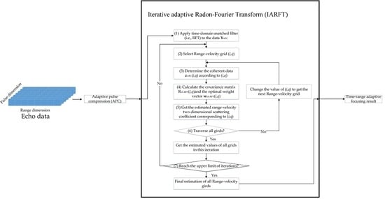
Since the essence of the APC method is the same as that of the IAA method [31], we can use APC method as a reference to estimate the covariance matrix according to the signal model of in an iterative way, and deduce the optimal weight vector of the IARFT method. Figure 4 is the flow chart of the IARFT method. According to Figure 4, the IARFT method mainly includes the following steps:
- (1)
- First, apply RFT to the data YAPC. The searching interval of range and searching interval of velocity have been discretized into NrNv range-velocity grids. Without considering the intra-pulse Doppler frequency, the discrete form of RFT in range-velocity two-dimensional parameter space is expressed as [46,47],where i and q are discrete variables referring to i-th range gird and q-th velocity grid respectively. r(i) = rC − ra/2 + iΔr, v(q) = −vmax + qΔv. represents the rounding approximation operation, and Hv(q)(m) is the Doppler filter bank [48,49],where is the wavelength of the carrier. The result of RFT is used as the initial estimation of all range-velocity grids’ scattering coefficients, so RFT needs to be applied at the beginning of the IARFT method.
- (2)
- Assign a value to the range-velocity grid (i,q). Since IARFT method needs to traverse all grids, grid (i,q) generally starts with grid (1,1) and ends with grid (Nr,Nv) in one iteration.
- (3)
- According to the range cell and velocity corresponding to the specific range-velocity grid (i,q), the trajectory within the CPI T is determined, and the coherent data is also determined.
- (4)
- IARFT method derives the optimal filter by constructing the cost function. According to MVDR criterion, the cost function of range-velocity grid (i,q) is defined as,
According to Equation (11), refers to all other range-velocity grids except the grid of interest. Blindly traversing the trajectories of all grids will cause a large number of indication vectors equal to zero vector and increase the computational cost. Considering v(q), v(k) [−vmax, vmax], once |r(j) − r(i)|> vmaxT, the trajectories corresponding to will not overlap with the trajectory corresponding to . Thus, we set Nc as,
Then we set matrix to satisfy,
According to Equations (11) and (22), can be expressed as,
Because it is assumed that the targets of different range-velocity grids are independent of each other and the targets are independent of the noise, is expressed as,
The noise is assumed to be additive Gaussian white noise, and the noise covariance matrix R(i,q) can be simplified as . Since Equation (16) requires,
So, we can get,
Thus, the optimal weight vector of IARFT method via MVDR criterion can be obtained as,
Note that is unknown, so we need to use the estimation instead. In the first iteration of IARFT method, the result of RFT method in step (1) needs to be used in Equation (27) as the initial estimated scattering coefficient of the range-velocity two-dimensional gird to calculate and .
- (5)
- Since the optimal weight vector is obtained, the estimated scattering coefficient of the range-velocity two-dimensional gird is,
- (6)
- Judge whether all the range-velocity grids have been traversed in this iteration. If no, assign another range-velocity grid as (i,q) and continue to estimate the scattering coefficient of the range-velocity two-dimensional gird (i,q) through Equations (27) and (28). If yes, we will get the estimated scattering coefficients of all grids in this iteration and jump to step (7).
- (7)
- Judge whether the upper limit of iteration LoopIARFT has been reached in this iteration. If no, jump to step (2) to start a new iteration, and continue to estimate the scattering coefficient of the range-velocity two-dimensional gird (i,q). If yes, the result obtained in step (6) can be the final estimation of the range-velocity two-dimensional scattering coefficients in IARFT method.
After LoopIARFT iterations, IARFT method can suppress the velocity sidelobes of strong targets, and obtain a better range-velocity two-dimensional output, which is the final output of APC-IARFT method.
5. Discussion of IARFT Method
Iterative operation is the key content of APC-IARFT method. The conditions of terminating iterations and the computational cost of one iteration in APC method have been analyzed in [27,32], so the conclusion will not be repeated here. The IARFT method is a method first proposed in this paper. Therefore, this section focuses on IARFT method and analyzes its conditions of terminating the iterations and computational cost in one iteration.
5.1. Conditions of Terminating the Iterations in IARFT Method
In order to obtain a good energy focusing performance, the number of iterations in IARFT method, i.e., LoopIARFT should be no less than 6 times. The more the number of iterations, the better convergence and range-velocity sidelobes suppression of IARFT method. However, increasing LoopIARFT will affect the computational cost of the whole algorithm, and the output of IARFT method will eventually tends to be stable after multiple iterations. Therefore, when the modulus of the difference between the result of the current iteration and the result of the previous iteration is less than the arranged threshold ThIARFT, the iterations of IARFT method can end.
5.2. Computational Cost in One Iteration of IARFT Method
Since IARFT method includes multiple iterations, the computational cost of an iteration is analyzed here. Using the RFT method to search data in pulse trains to realize time-dimension matched filter is equivalent to one iteration, so its computational cost is Np complex multiplication and Np − 1 complex addition for each range-velocity gird and RFT requires O(Np) operations. In contrast, for each range-velocity gird in one iteration of the IARFT method, firstly we need to calculate the Np × 1-dimensional indication vector with the trajectories of the adjacent range-velocity girds according to Equation (22), which requires 2NcNvNp complex multiplication and Np complex addition. Secondly, Np × Np-dimensional covariance matrix is solved according to Equation (24), which requires 2NcNv(Np2) complex multiplication and Np complex addition. Thirdly, the inverse matrix is solved according to the covariance matrix, which requires Np3/3 complex number multiplication. Finally, the weight vector is calculated according to the covariance matrix and the steering vector, and the scattering coefficient is estimated. The whole process in one iteration requires O(Np3) operations. Therefore, the computational cost of the IARFT method is indeed higher than that of the conventional RFT method [6].
6. Experimental Results
This section introduces some numerical simulation experiments to prove the effectiveness of the IARFT method in suppressing velocity sidelobes and effectiveness of the APC-IARFT method in suppressing range-velocity sidelobes by comparing with other methods. The methods involved in the comparison include cascade of conventional pulse compression and the RFT method, cascade of conventional pulse compression and the ARFT method, cascade of conventional pulse compression and the IARFT method and the APC-IARFT method (for convenience of description, the first three methods are directly referred to as the RFT method, ARFT method and IARFT method). The parameters of the radar system are set as follows: carrier frequency is 1 GHz, pulse repetition frequency (PRF) is 1000 Hz, bandwidth B of linear frequency modulation signal is 15 MHz, pulse width Tp is 5 μs. Sampling frequency fs = 30 Mhz (so N = Tp;∙fs = 150). Since the coherence between pulses cannot be guaranteed by staring at the high-speed target for a long CPI T, the CPI T is set as 0.05 s (i.e., Np is 50). The center rC of the search area is located at 100 km, vmax = 540 m/s, and the range of the search area ra = 300 m. rmax = 327 m, Δr = 5 m, Nr = 60, Δv = 3 m/s, Nv = 360. The power of noise is set as −20 dB. The number of iterations in the APC method is set as 2 times, and the number of iterations in the IARFT method is set as 6 times. In this experiment, two kinds of average peak sidelobe level (APSL) between the target and the neighboring grids are set to help analyze the performance of different methods, which are named as APSL2D and APSLv respectively. The calculation rule of APSL2D is the ratio between amplitude of grid (i,q) and average amplitude of girds whose range is within [rC − ra/2, rC + ra/2], and velocity is within v(q) ± 75 m/s (75 m/s is the velocity corresponding to PRF/2 in the experiment) meanwhile,
The calculation rule of APSLv is is the ratio between amplitude of grid (i,q) and average amplitude of girds whose velocity is within v(q) ± 75 m/s,
where is the estimatied scattering coefficient of grid (i,q), and is the estimatied scattering coefficient of neighboring grid. mean(·) is the mean function. Both APSL2D and APSLv require multiple experiments to calculate the average values.
6.1. Scenario 1: Point Target with High Signal-To-Noise Ratio
There are 2 targets set in Scenario 1, whose basic information is listed in Table 1.
Figure 5 shows the two-dimensional stereogram of the four methods’ range-velocity output. It should be noted that the searching interval of velocity [−vmax, vmax] used in all the above methods exceeds the range of maximum unambiguous velocity (the range of maximum unambiguous velocity corresponding to PRF in the scenarios is 150 m/s), so the energy will be focused every 150 m/s in velocity dimension, which is the reason for the blind speed sidelobes (BSSL) [7]. However, the data searched by other blind speeds is inaccurate and cannot be completely coherent, so the BSSL cannot achieve the focusing result comparable to the main lobe of the target. In Figure 5a, the main lobe and the BSSL of Target 1 can be clearly seen. The sidelobes of target 1 completely cover the main lobe of Target 2. It can also be clearly seen that there is a certain low-velocity region around the main lobe, and the suppression of velocity sidelobes is relatively obvious in this low-velocity region. The suppression of velocity sidelobes in the low-velocity region is due to the fact that a target with the velocity in the low-velocity region will not move across the range cell during the CPI T. In addition, the target’s velocity is different from the velocity in the low-velocity region, and the phase of time-dimension steering vector corresponding to the velocity in the low-velocity region does not match Target 1’s velocity, so the velocity in the low-velocity region cannot realize focusing. It is known that Δr = 5 m, T = 0.05 s in the experiment, and the range value given by the grid refers to the actual range of the grid’s center. Δr/T = 100 m/s, so ARC walking occurs when the target’s velocity is higher than 100 m/s, and the low-velocity region where the velocity sidelobes are suppressed in Figure 5a is precisely [−100 m/s, 100 m/s]. In Figure 5b, the limited number of coherent pulses affects the output of ARFT method. At the same time, due to the processing of clutter’s covariance matrix, the energy at the velocity of Target 1 is excavated to form a notch. The output of IARFT method in Figure 5c is better comparing with those of RFT and ARFT. IARFT suppresses the velocity sidelobes of Target 1, so we can distinguish the main lobe of Target 2 (the position marked by the red ellipse in Figure 5c). However, the BSSL of Target 1 in Figure 5c is still very obvious. The APC-IARFT method is the best among the four methods. The velocity sidelobes and BSSL of Target 1 are suppressed simultaneously in Figure 5d.
The range-velocity two-dimensional plan output processed by the RFT, ARFT, IARFT, and APC-IARFT methods is shown in Figure 6. We can compare the differences between these methods more clearly in Figure 6. Obviously, IARFT and APC-IARFT methods suppress the velocity sidelobes as much as possible and distinguish Target 2. The APC-IARFT method further suppresses range sidelobes comparing with the IARFT method. Figure 7 shows the comparison of output in velocity dimension at the range cell where the target is located. The velocity-dimension output of the RFT method does achieve sidelobes suppression within [−100 m/s, 100 m/s], while the sidelobes at other velocities and the BSSL of Target 1 mask Target 2. The ARFT method does not achieve effective focusing in the velocity dimension. The IARFT and APC-IARFT methods suppress the velocity sidelobes better in Figure 7 and the APC-IARFT method is the best of the methods.
The calculated APSL2D and APSLv of the targets set in Scenario 1 are listed in Table 2, which also illustrate that APC-IARFT and IARFT methods are better than the RFT and ARFT methods, and the APC-IARFT method is the best in this scenario.
6.2. Scenario 2: Dense Target Scenario
Multiple moving targets are set in this Scenario, and the initial positions are still located at 100 km. The radial velocity, Doppler frequency and initial SNR of each moving target are shown in Table 3.
Figure 8 shows the two-dimensional stereogram of the four methods’ range-velocity output. In Figure 8a, the main lobe and BSSL of Target 1 can still be clearly seen, and the suppression of velocity sidelobes around the main lobe is obvious in the low-velocity region of [−100 m/s, 100 m/s]. Because Target 1 is relatively strong compared with other targets, its BSSL masks the main lobes of other targets. In Figure 8b, the limited number of coherent pulses still affects the output of the ARFT method. Similar to Figure 5b, due to the processing of clutter’s covariance matrix, the energy at the velocity of Target 1 in Figure 8b is also excavated to form a notch. The performance of focusing in Figure 8c is very obvious. The IARFT method suppresses the velocity sidelobes, and we can basically distinguish the positions of the other three targets (the positions marked by the red ellipses in Figure 8c). However, the BSSL of Target 1 still exist in Figure 8c, which will also affect other targets.
In the same experimental scenario, cascade of APC and IARFT will get a better output. Different from conventional pulse compression, the range sidelobes of the targets is suppressed by the APC method, which can better reduce the influence of the range sidelobes on other weak targets. The performance of focusing in Figure 8d is more obvious than that in Figure 8c, which not only suppresses the range sidelobes and velocity sidelobes, but also significantly suppresses the BSSL of Target 1. So, we can directly distinguish the positions of the other three targets (the positions marked by the red ellipses in Figure 8d).
The range-velocity two-dimensional plan output of the RFT, ARFT, IARFT, and APC-IARFT methods is shown in Figure 9. The differences between these methods can be seen more clearly in Figure 9. Obviously, the IARFT method suppresses the velocity sidelobes as much as possible and we can basically distinguish the positions of three weak targets. Although the BSSL of Target 1 is suppressed by IARFT to some extent, it still exists. Especially in the output of the APC-IARFT method, the range-velocity sidelobes and BSSL are almost suppressed, and nearly only the target point can be seen.
Figure 10 shows the comparison of velocity-dimension output at the range cell where the target is located. The velocity-dimension output of the RFT method still achieves velocity sidelobes suppression within [−100 m/s, 100 m/s], while the sidelobes and the BSSL of Target 1 mask other weak targets. The velocity-dimension output in ARFT method does not achieve effective focusing. Figure 10 intuitively shows that the IARFT method effectively suppresses the velocity sidelobes, so that the main lobe of weak targets can be distinguished. However, the range sidelobes of targets and the BSSL of Target 1 are still obvious in the output of the IARFT method when comparing with that of the APC-IARFT method. Thus, the APC-IARFT method is still the best of the methods and we can almost only see the main lobed of the targets in its output.
The calculated APSL2D and APSLv of the targets set in Scenario 2 are listed in Table 4. We can also see that the APC-IARFT and IARFT methods are better than the RFT and ARFT methods, and the APC-IARFT method is the best in this scenario.
6.3. Scenario 3: Point Targets with Low SNR and High Speed
In Scenario 3, two fast-moving point targets are set, and their initial position is located at 100 km. The radial velocity, Doppler frequency, and initial SNR of each moving target are shown in Table 5.
Figure 11 shows the two-dimensional stereogram of range-velocity output. In Figure 11a, we can distinguish the main lobe and BSSL of the point targets. In Figure 11b, the output of the ARFT method is similar to that of the RFT method, but velocity-dimension sidelobes are more serious than that in Figure 11a due to the processing of covariance matrix in the ARFT method. It can be seen that for point targets with low SNR that the output of IARFT method is consistent with that of the RFT method. However, the output of the APC-IARFT method is intuitively better than that of the IARFT method. The range-velocity two-dimensional plan output of the RFT, ARFT, IARFT and APC-IARFT methods is shown in Figure 12. The relative position relationship between the main lobes and BSSL in the output of different methods can be more clearly seen in Figure 12. Due to the small number of coherent pulses in the scene, it can be seen from the output of the ARFT method that the clutter’s covariance matrix makes more obvious velocity sidelobes appear in the velocity dimension.
Figure 13 shows the comparison of velocity-dimension output at the range cell where the targets are located. The velocity-dimension output of the IARFT method, and the RFT method is basically the same, so their curves overlap with each other. In the ARFT method, there are more obvious sidelobes in the velocity dimension. The APC-IARFT method further suppress the velocity sidelobes on the basis of IARFT method. The calculated APSL2D and APSLv of the targets set in Scenario 4 are listed in Table 6. According to the data comparison in Table 6, the APC-IARFT method is still the best among the four methods.
6.4. Scenario 4: Point Target in Clutter Background
In order to illustrate the performance of the APC-IARFT method in the clutter background, two targets are set in Scenario 4, whose information is listed in Table 7. Suppose the clutter is uniform and stationary, and its clutter-to-noise ratio (CNR) is set as 30 dB. Clutter’s amplitude obeys Gaussian distribution, and the Doppler spectral density function is Gaussian spectrum. The center of clutter’s Gaussian spectrum is 0 Hz, and the variance of velocity is 1.5 m/s, so the width of Gaussian spectrum is 10 Hz.
In the clutter background, the energy of clutter is also accumulated by the RFT method. So, we can see that after the focusing, the amplitude of clutter is higher than that of noise in Figure 14a. However, the amplitude of clutter is lower than that of Target 1 due to the coherence of the target’s echo. The ARFT method is beneficial to the clutter background, and the clutter is suppressed in Figure 14b. Because Target 1’s Doppler frequency is located in clutter’s spectrum, the main lobes of Target 1 and Target 2 are excavated by the processing of clutter’s covariance matrix. The IARFT method needs to utilize the output of the RFT method as the initial estimation of the range-velocity two-dimensional scattering coefficient. In the clutter background, although the velocity sidelobes of clutter can be suppressed, the IARFT method will also integrate clutter’s energy like the RFT method. In Figure 14a,c,d clutter is not suppressed, but the ability of the IARFT method to suppress velocity sidelobes in clutter background is still stronger than that of the RFT method by comparing Figure 14c with Figure 14a.
Comparing Figure 14d with Figure 14c, the ability of APC to suppress range sidelobes and the ability of the IARFT method to suppress velocity sidelobes are still obvious. However, we find another problem through comparison. Although the APC method suppresses range sidelobes, it may change the range-dimension statistical characteristics of the clutter. After APC’s processing, the clutter becomes stronger than that in the IARFT method. In this experimental background, although the clutter in the output of the APC-IARFT method diffuses in the range dimension, the ability of the APC-IARFT method to suppress range-velocity sidelobes is still the best. According to the comparison of targets’ range-velocity sidelobes in Figure 15 and the comparison of targets’ velocity sidelobes in Figure 16, the results can still verify the ability of IARFT method to suppress velocity sidelobes and the ability of the APC-IARFT method to suppress range-velocity sidelobes.
The calculated APSL2D and APSLv of the targets set in Scenario 4 are listed in Table 8. In the calculation of APSL2D, the performance of the IARFT method is the best. We can see that the APC method does change the amplitude of clutter in Figure 15. So, the values in the APC-IARFT method are lower than those in the IARFT method. In the calculation of APSLv, it is obvious that the IARFT method is also optimal from the aspect of numerical comparison. When calculating APSLv of Target 1, the value of the APC-IARFT method is close to those of the IARFT and RFT method. Although the output of the APC-IARFT method is not as good as that that of cascade of matched filter and IARFT method in this clutter background, it is still better than that of conventional RFT and ARFT when calculate APSLv of Target 2, which also illustrates the advantage of the IARFT method. In addition, when calculating APSLv of Target 2, the value in the APC-IARFT method is better than that in the IARFT method. This can also illustrate the ability of the APC-IARFT method to suppress velocity sidelobes.
7. Conclusions
By considering the coherent integration as focusing, we consider pulse compression as range-dimensional focusing and long-time coherent integration as long-time focusing. However, the matched filter has problems such as range sidelobes. RFT belongs to standard time-dimension matched filter, which will cause velocity sidelobes of strong targets. The range-velocity sidelobes caused by matched filter and RFT will mask other weak targets and affect the energy focusing and the subsequent signal processing processes such as target detection and tracking. To achieve better focusing, this paper studies the adaptive focusing of two dimensions of time and range. Firstly, the idea of the iterative adaptive approach is applied to long-time focusing, and a long-time adaptive focusing method based on iterative adaptive RFT (IARFT) is designed. Further, in order to solve the problem of two-dimensional sidelobes masking, this paper proposes a time-range adaptive focusing method (APC-IARFT for short) based on APC and IARFT. By cascading the APC method and IARFT method, the range-velocity sidelobes can be adaptively suppressed under the range-velocity grid without additional prior information.
In addition, the computational cost of the IARFT method is high, and the research on its fast implementation will be an important part of future research.
It should be noted that the IARFT method suppress the velocity sidelobes, but it does not completely suppress the clutter. In order to suppress the clutter, we think that the most feasible method is to estimate the clutter’s covariance matrix, and whiten the echo data before IARFT method. Another method is to add the estimation of clutter’s covariance matrix, i.e., add the clutter’s covariance matrix to the covariance matrix calculation of IARFT method (i.e., Equation (24) in Section 5.2).
Furthermore, we also found that there are still some problems if the IARFT method is carried out after the APC method in the clutter background through Section 6.4. We think that the APC method may affect the statistical characteristics of clutter in the cascaded processing. The next research content is to integrate the APC method and IARFT method into the multi-dimensional joint processing to realize the joint processing of the two methods, which can further expand the dimensions and manners of processing, and achieve the optimal processing in coherent integration of high-speed weak targets.
Author Contributions
Conceptualization, J.G., J.P. and B.C.; methodology, J.P., Y.H. and B.C.; software, J.P., B.C. and X.C.; validation, J.P., B.C. and X.C.; formal analysis, J.P.; investigation, X.C.; resources, X.C.; data curation, Y.H.; writing—original draft preparation, B.C.; writing—review and editing, J.P.; visualization, J.P.; supervision, Y.H.; project administration, J.G.; funding acquisition, J.G. All authors have read and agreed to the published version of the manuscript.
Funding
This research was funded by National Natural Science Foundation of China, grant number 62222120, 61871391, Shandong Provincial Natural Science Foundation, grant number ZR2021YQ43, Youth Innovation and Technology Support Plan of Universities in Shandong Province, grant number 2019KJN026.
Data Availability Statement
Not applicable.
Conflicts of Interest
The authors declare no conflict of interest.
References
- Li, Y.; Zeng, T.; Long, T. Range migration compensation and Doppler ambiguity resolution by Keystone transform. In Proceedings of the International Conference on Radar, Shanghai, China, 16–19 October 2006. [Google Scholar] [CrossRef]
- Kong, L.; Li, X.; Cui, G.; Yi, W.; Yang, Y. Coherent integration algorithm for a maneuvering target with High-Order range migration. IEEE Trans. Signal Process. 2015, 63, 4474–4486. [Google Scholar] [CrossRef]
- Li, X.; Cui, G.; Yi, W.; Kong, L. Manoeuvring target detection based on keystone transform and Lv’s distribution. IET Radar Sonar Navig. 2016, 10, 1234–1242. [Google Scholar] [CrossRef]
- Li, X.; Kong, L.; Cui, G.; Yi, W. CLEAN-based coherent integration method for high-speed multi-targets detection. IET Radar Sonar Navig. 2016, 10, 1671–1682. [Google Scholar] [CrossRef]
- Reed, I.S.; Gagliardi, R.M.; Stotts, L.B. Optical moving target detection with 3-D matched filtering. IEEE Trans. Aerosp. Electron. Syst. 1998, 24, 327–335. [Google Scholar] [CrossRef]
- Xu, J.; Yu, J.; Peng, Y.; Xia, X. Radon-Fourier Transform for Radar Target Detection, I: Generalized Doppler filter bank. IEEE Trans. Aerosp. Electron. Syst. 2011, 47, 1186–1202. [Google Scholar] [CrossRef]
- Xu, J.; Yu, J.; Peng, Y.; Xia, X. Radon-Fourier Transform for Radar Target Detection (II): Blind speed sidelobe suppression. IEEE Trans. Aerosp. Electron. Syst. 2011, 47, 2473–2489. [Google Scholar] [CrossRef]
- Xu, J.; Yu, J.; Peng, Y.; Xia, X. Radon-Fourier Transform for Radar Target Detection (III): Optimality and fast implementations. IEEE Trans. Aerosp. Electron. Syst. 2012, 48, 991–1004. [Google Scholar] [CrossRef]
- Xu, J.; Xia, X.; Peng, S.; Yu, J.; Peng, Y.; Qian, L. Radar Maneuvering Target Motion Estimation Based on Generalized Radon-Fourier Transform. IEEE Trans. Signal Process. 2012, 60, 6190–6201. [Google Scholar] [CrossRef]
- Qian, L.; Xu, J.; Xia, X.; Sun, W.; Long, T.; Peng, Y. Fast implementation of generalized Radon-Fourier transform for manoeuvring radar target detection. Electron. Lett. 2012, 48, 1427–1428. [Google Scholar] [CrossRef]
- Qian, L.; Xu, J.; Xia, X.; Sun, W.; Long, T.; Peng, Y. Wideband-scaled Radon-Fourier transform for high-speed radar target detection. IET Radar Sonar Navig. 2014, 8, 501–512. [Google Scholar] [CrossRef]
- Xu, J.; Yu, J.; Peng, Y.; Xia, X.; Long, T. Space-time Radon-Fourier transform and applications in radar target detection. IET Radar Sonar Navig. 2012, 6, 846–857. [Google Scholar] [CrossRef]
- Xu, J.; Peng, Y.; Xia, X.; Long, T.; Mao, E. Radar Signal Processing Method of Space-Time-Frequency Focus-Before-Detects. J. Radars 2014, 3, 129–141. [Google Scholar] [CrossRef]
- Xu, J.; Zhou, X.; Qian, L.; Xia, X.; Long, T. Hybrid integration for highly maneuvering radar target detection based on generalized radon-fourier transform. IEEE Trans. Aerosp. Electron. Syst. 2016, 52, 2554–2561. [Google Scholar] [CrossRef]
- Xu, J.; Peng, Y.; Xia, X.; Farina, A. Focus-before-detection radar signal processing: Part I—Challenges and methods. IEEE Aerosp. Electron. Syst. Mag. 2017, 32, 48–59. [Google Scholar] [CrossRef]
- Xu, J.; Peng, Y.; Xia, X.; Long, T.; Mao, E.; Farina, A. Focus-before-detection radar signal processing: Part II—Recent developments. IEEE Aerosp. Electron. Syst. Mag. 2018, 33, 34–49. [Google Scholar] [CrossRef]
- Chen, X.; Guan, J.; Liu, N.; He, Y. Maneuvering target detection via Radon-Fractional Fourier Transform-Based Long-Time coherent integration. IEEE Trans. Signal Process. 2014, 62, 939–953. [Google Scholar] [CrossRef]
- Chen, X.; Guan, J.; Huang, Y.; Liu, N.; He, Y. Radon-Linear canonical ambiguity Function-Based detection and estimation method for marine target with micromotion. IEEE Trans. Geosci. Remote Sens. 2015, 53, 2225–2240. [Google Scholar] [CrossRef]
- Xu, J.; Yan, L.; Zhou, X.; Long, T.; Xia, X.; Wang, Y.; Farina, A. Adaptive Radon–Fourier transform for weak radar target detection. IEEE Trans. Aerosp. Electron. Syst. 2018, 54, 1641–1663. [Google Scholar] [CrossRef]
- You, P.; Ding, Z.; Qian, L.; Li, M.; Zhou, X.; Liu, W.; Liu, S. A motion parameter estimation method for radar maneuvering target in gaussian clutter. IEEE Trans. Signal Process. 2019, 67, 5433–5446. [Google Scholar] [CrossRef]
- Ding, D.; You, P.; Qian, L.; Zhou, X.; Liu, S.; Long, T. A subspace hybrid integration method for High-Speed and maneuvering target detection. IEEE Trans. Aerosp. Electron. Syst. 2020, 56, 630–644. [Google Scholar] [CrossRef]
- Schmidt, R. Multiple emitter location and signal parameter estimation. IEEE Trans. Antennas Propag. 1986, 34, 276–280. [Google Scholar] [CrossRef] [Green Version]
- Barabell, A. Improving the resolution performance of eigenstructure-based direction-finding algorithms. In Proceedings of the IEEE International Conference on Acoustics, Speech, and Signal Processing (ICASSP ’83), Boston, MA, USA, 14–16 April 1983. [Google Scholar] [CrossRef]
- Paulraj, A.; Roy, R.; Kailath, T. A subspace rotation approach to signal parameter estimation. Proc. IEEE 1986, 74, 1044–1046. [Google Scholar] [CrossRef]
- Blunt, S.D.; Chan, T.; Gerlach, K. A new framework for direction-of-arrival estimation. In Proceedings of the 2008 5th IEEE Sensor Array and Multichannel Signal Processing Workshop, Darmstadt, Germany, 21–23 July 2008. [Google Scholar] [CrossRef]
- Blunt, S.D.; Chan, T.; Gerlach, K. Robust DOA estimation: The reiterative superresolution (RISR) algorithm. IEEE Trans. Aerosp. Electron. Syst. 2011, 47, 332–346. [Google Scholar] [CrossRef]
- Blunt, S.D.; Gerlach, K. Adaptive pulse compression via MMSE estimation. IEEE Trans. Aerosp. Electron. Syst. 2006, 42, 572–584. [Google Scholar] [CrossRef]
- Higgins, T.; Blunt, S.D.; Shackelford, A.K. Space-Range Adaptive Processing for Waveform-Diverse Radar Imaging. In Proceedings of the 2010 IEEE Radar Conference, Arlington, VA, USA, 10–14 May 2010. [Google Scholar] [CrossRef]
- Higgins, T.; Blunt, S.D.; Shackelford, A.K. Time-Range Adaptive Processing for pulse agile radar. In Proceedings of the 2010 International Waveform Diversity and Design Conference, Niagara Falls, ON, Canada, 8–13 August 2010. [Google Scholar] [CrossRef] [Green Version]
- Yardibi, T.; Li, J.; Stoica, P.; Xue, M.; Baggeroer, A.B. Source localization and sensing: A nonparametric iterative adaptive approach based on weighted least squares. IEEE Trans. Aerosp. Electron. Syst. 2010, 46, 425–443. [Google Scholar] [CrossRef]
- Chen, B.; Huang, Y.; Chen, X.; Guan, J. Space-Time-Range Adaptive Processing for MIMO Radar Imaging. In Proceedings of the International Conference on Radar, Brisbane, QLD, Australia, 27–31 August 2018; pp. 1–6. [Google Scholar] [CrossRef]
- Higgins, T.; Blunt, S.D.; Gerlach, K. Gain-constrained adaptive pulse compression via an MVDR framework. In Proceedings of the 2009 IEEE Radar Conference, Pasadena, CA, USA, 4–8 May 2009. [Google Scholar] [CrossRef]
- Kay, S.M. Fundamentals of Statistical Signal Processing: Estimation Theory; Prentice-Hall: Upper Saddle River, NJ, USA, 1993; pp. 219–286, 344–350. [Google Scholar]
- Chen, X.; Yu, X.; Huang, Y.; Guan, J. Adaptive Clutter Suppression and Detection Algorithm for Radar Maneuvering Target With High-Order Motions Via Sparse Fractional Ambiguity Function. IEEE J. Sel. Top. Appl. Earth Obs. Remote Sens. 2020, 13, 1515–1526. [Google Scholar] [CrossRef]
- Chen, X.; Zhang, H.; Song, J.; Guan, J.; Li, J.; He, Z. Micro-Motion Classification of Flying Bird and Rotor Drones via Data Augmentation and Modified Multi-Scale CNN. Remote Sens. 2022, 14, 1107. [Google Scholar] [CrossRef]
- Ning, C.; Tian, J.; Li, K.; Wu, S. Modified Adaptive Pulse Compression Algorithm for Targets With Range-Straddling. IEEE Trans. Aerosp. Electron. Syst. 2021, 57, 3057–3070. [Google Scholar] [CrossRef]
- Ma, J.; Li, K.; Tian, J.; Long, X.; Wu, S. Fast Sidelobe Suppression Based on Two-Dimensional Joint Iterative Adaptive Filtering. IEEE Trans. Aerosp. Electron. Syst. 2021, 57, 3463–3478. [Google Scholar] [CrossRef]
- Pei, J.; Huang, Y.; Guan, J.; Cai, M.; Chen, B.; Chen, X. Robust Adaptive Pulse Compression Method Based on Two-Stage Phase Compensation. IEEE Trans. Geosci. Remote Sens. 2022, 60, 5104918. [Google Scholar] [CrossRef]
- Tan, X.; Roberts, W.; Li, J.; Stoica, P. Range-Doppler Imaging Via a Train of Probing Pulses. IEEE Trans. Signal Process. 2009, 57, 1084–1097. [Google Scholar] [CrossRef]
- Chen, X.; Liu, N.; Wang, G.; Guan, J. Radar Detection Method for Moving Target Based on Radon-Fourier Fractional Fourier Transform. Acta Electron. Sin. 2014, 42, 1074–1080. [Google Scholar] [CrossRef]
- Duan, Y.; Shang, Z.; Tan, X.; Qu, Z.; Li, Z. Fast implementation of RFT for radar hypersonic targets detection. Syst. Eng. Electron. 2018, 40, 1233–1240. [Google Scholar] [CrossRef]
- Qian, L.; Xu, J.; Sun, W.; Peng, Y. Blind Speed Side Lobe Suppression in Radon-Fourier Transform Based on Radar Pulse Recurrence Interval Design. J. Electron. Inf. Technol. 2012, 34, 2608–2614. [Google Scholar] [CrossRef]
- Qian, L.; Xu, J.; Sun, W.; Peng, Y. Wideband Time-space Radon-Fourier Transform for High-speed and Weak Target Detection. J. Electron. Inf. Technol. 2013, 35, 15–23. [Google Scholar] [CrossRef]
- Chen, Q.; Fu, C.; Liu, J.; Wu, S. Coherent Integration Based on Random Pulse Repetition Interval Radon-Fourier Transform. J. Electron. Inf. Technol. 2015, 37, 1085–1090. [Google Scholar] [CrossRef]
- Wu, Z.; Fu, W.; Su, T.; Zheng, J. High Speed Radar Target Detection Based on Fast Radon-Fourier Transform. J. Electron. Inf. Technol. 2012, 34, 1866–1871. [Google Scholar] [CrossRef]
- Qian, L.; Xu, J.; Sun, W.; Peng, Y. Blind Speed Side Lobe Suppression inRadon-Fourier Transform Based on MIMO Radar with Multi-carrier Frequency. Acta Aeronaut. Astronaut. Sin. 2013, 34, 1181–1190. [Google Scholar] [CrossRef]
- Lin, C.; Huang, C.; Su, Y. Target Integration and Detection with the Radon-Fourier Transform for Bistatic Radar. J. Radars 2016, 5, 526–530. [Google Scholar] [CrossRef]
- Qian, L.; Xu, J.; Hu, G. Long-time Integration of a Multiwaveform for Weak Target Detection in Non-cooperative Passive Bistatic Radar. J. Radars 2017, 6, 259–266. [Google Scholar] [CrossRef]
- Qian, L.; Xu, J.; Sun, W.; Peng, Y. A Study on Wideband Radon-Fourier Transform and Its Fast Implementation Based on CZT. Mod. Radar 2013, 4, 39–44. [Google Scholar] [CrossRef]
Figure 1.
The across range cells (ARC) walk of a target.

Figure 2.
Schematic diagram of targets’ motion trajectories overlapping and affecting each other in the search area.
Figure 2.
Schematic diagram of targets’ motion trajectories overlapping and affecting each other in the search area.

Figure 3.
Schematic diagram of indication vector obtained by targets’ motion trajectories overlapping.
Figure 3.
Schematic diagram of indication vector obtained by targets’ motion trajectories overlapping.

Figure 4.
Flow chart of the IARFT method.

Figure 5.
Stereogram output of four methods in Scenario 1. (a) Output of RFT; (b) Output of ARFT; (c) Output of IARFT; (d) Output of APC-IARFT.
Figure 5.
Stereogram output of four methods in Scenario 1. (a) Output of RFT; (b) Output of ARFT; (c) Output of IARFT; (d) Output of APC-IARFT.

Figure 6.
Plan output of four methods in Scenario 1.

Figure 7.
Velocity-dimension output of four methods in Scenario 1.

Figure 8.
Stereogram output of four methods in Scenario 2. (a) Output of RFT; (b) Output of ARFT; (c) Output of IARFT; (d) Output of APC-IARFT.
Figure 8.
Stereogram output of four methods in Scenario 2. (a) Output of RFT; (b) Output of ARFT; (c) Output of IARFT; (d) Output of APC-IARFT.


Figure 9.
Plan output of four methods in Scenario 2.

Figure 10.
Velocity-dimension output of four methods in Scenario 2.

Figure 11.
Stereogram output of four methods in Scenario 3: (a) Output of RFT; (b) Output of ARFT; (c) Output of IARFT; (d) Output of APC-IARFT.
Figure 11.
Stereogram output of four methods in Scenario 3: (a) Output of RFT; (b) Output of ARFT; (c) Output of IARFT; (d) Output of APC-IARFT.

Figure 12.
Plan output of four methods in Scenario 3.

Figure 13.
Velocity-dimension output of four methods in Scenario 3.

Figure 14.
Stereogram output of four methods in Scenario 4. (a) Output of RFT; (b) Output of ARFT; (c) Output of IARFT; (d) Output of APC-IARFT.
Figure 14.
Stereogram output of four methods in Scenario 4. (a) Output of RFT; (b) Output of ARFT; (c) Output of IARFT; (d) Output of APC-IARFT.


Figure 15.
Plan output of four methods in Scenario 4.

Figure 16.
Velocity-dimension output of four methods in Scenario 4.


Table 1.
Basic information of the targets set in Scenario 1.
| Target No. | Initial Position | Radial Velocity | Doppler Frequency | Signal-To-Noise Ratio (SNR) |
|---|---|---|---|---|
| 1 | 100 km | 15 m/s | 100 Hz | 40 dB |
| 2 | 100 km | 420 m/s | 3400 Hz | 5 dB |
Table 2.
APSL2D and APSLv of the targets set in Scenario 1.
| RFT | ARFT | IARFT | APC-IARFT | |
|---|---|---|---|---|
| APSL2D of Target 1 | 71.36 dB | 3.14 dB | 69.98 dB | 75.05 dB |
| APSL2D of Target 2 | 27.86 dB | 13.97 dB | 22.32 dB | 39.79 dB |
| APSLv of Target 1 | 60.06 dB | −13.21 dB | 56.85 dB | 63.90 dB |
| APSLv of Target 2 | 3.66 dB | −1.47 dB | 10.26 dB | 23.54 dB |
Table 3.
Basic information of the targets set in Scenario 2.
| Target No. | Initial Position | Radial Velocity | Doppler Frequency | Signal-To-Noise Ratio (SNR) |
|---|---|---|---|---|
| 1 | 100 km | 15 m/s | 100 Hz | 40 dB |
| 2 | 100 km | 210 m/s | 1400 Hz | 10 dB |
| 3 | 100 km | 339 m/s | 2260 Hz | 5 dB |
| 4 | 100 km | 400 m/s | 2667 Hz | 0 dB |
Table 4.
APSL2D and APSLv of the targets set in Scenario 2.
| RFT | ARFT | IARFT | APC-IARFT | |
|---|---|---|---|---|
| APSL2D of Target 1 | 73.39 dB | 5.99 dB | 69.02 dB | 73.16 dB |
| APSL2D of Target 2 | 23.10 dB | 27.05 dB | 36.72 dB | 42.82 dB |
| APSL2D of Target 3 | 22.55 dB | 24.31 dB | 29.67 dB | 37.56 dB |
| APSL2D of Target 4 | 15.57 dB | 26.41 dB | 23.70 dB | 30.46 dB |
| APSLv of Target 1 | 53.92 dB | −13.71 dB | 52.21 dB | 62.23 dB |
| APSLv of Target 2 | −8.18 dB | 1.16 dB | 24.04 dB | 31.38 dB |
| APSLv of Target 3 | −6.94 dB | 0.61 dB | 18.29 dB | 25.73 dB |
| APSLv of Target 4 | −5.63 dB | 7.06 dB | 13.34 dB | 18.60 dB |
Table 5.
Basic information of the targets set in Scenario 3.
| Target No. | Initial Position | Radial Velocity | Doppler Frequency | SNR |
|---|---|---|---|---|
| 1 | 100 km | 480 m/s | 3200 Hz | 0 dB |
| 2 | 100 km | 510 m/s | 3400 Hz | 0 dB |
Table 6.
APSL2D and APSLv of the targets set in Scenario 3.
| RFT | ARFT | IARFT | APC-IARFT | |
|---|---|---|---|---|
| APSL2D of Target 1 | 30.99 dB | 25.08 dB | 30.99 dB | 37.34 dB |
| APSL2D of Target 2 | 31.23 dB | 27.95 dB | 31.23 dB | 37.14 dB |
| APSLv of Target 1 | 19.84 dB | 13.37 dB | 19.85 dB | 28.98 dB |
| APSLv of Target 2 | 19.08 dB | 15.84 dB | 19.09 dB | 28.41 dB |
Table 7.
Basic information of the targets set in Scenario 4.
| Target No. | Initial Position | Radial Velocity | Doppler Frequency | SNR |
|---|---|---|---|---|
| 1 | 100 km | 15 m/s | 100 Hz | 30 dB |
| 2 | 100 km | 210 m/s | 1400 Hz | 25 dB |
Table 8.
APSL2D and APSLv of the targets set in Scenario 4.
| RFT | ARFT | IARFT | APC-IARFT | |
|---|---|---|---|---|
| APSL2D of Target 1 | 48.95 dB | −6.60 dB | 49.19 dB | 38.52 dB |
| APSL2D of Target 2 | 42.51 dB | −7.39 dB | 43.22 dB | 33.11 dB |
| APSLv of Target 1 | 34.14 dB | −0.48 dB | 36.10 dB | 33.83 dB |
| APSLv of Target 2 | 23.05 dB | −12.68 dB | 29.13 dB | 29.67 dB |
Publisher’s Note: MDPI stays neutral with regard to jurisdictional claims in published maps and institutional affiliations. |
© 2022 by the authors. Licensee MDPI, Basel, Switzerland. This article is an open access article distributed under the terms and conditions of the Creative Commons Attribution (CC BY) license (https://creativecommons.org/licenses/by/4.0/).
Share and Cite
MDPI and ACS Style
Guan, J.; Pei, J.; Huang, Y.; Chen, X.; Chen, B. Time-Range Adaptive Focusing Method Based on APC and Iterative Adaptive Radon-Fourier Transform. Remote Sens. 2022, 14, 6182. https://doi.org/10.3390/rs14236182
AMA Style
Guan J, Pei J, Huang Y, Chen X, Chen B. Time-Range Adaptive Focusing Method Based on APC and Iterative Adaptive Radon-Fourier Transform. Remote Sensing. 2022; 14(23):6182. https://doi.org/10.3390/rs14236182
Chicago/Turabian StyleGuan, Jian, Jiazheng Pei, Yong Huang, Xiaolong Chen, and Baoxin Chen. 2022. "Time-Range Adaptive Focusing Method Based on APC and Iterative Adaptive Radon-Fourier Transform" Remote Sensing 14, no. 23: 6182. https://doi.org/10.3390/rs14236182
Note that from the first issue of 2016, this journal uses article numbers instead of page numbers. See further details here.