
Efficient SfM for Large-Scale UAV Images Based on Graph-Indexed BoW and Parallel-Constructed BA Optimization

1
State Key Laboratory of Information Engineering in Surveying, Mapping and Remote Sensing, Wuhan University, Wuhan 430072, China
2
School of Computer Science, China University of Geosciences, Wuhan 430074, China
*
Author to whom correspondence should be addressed.
Remote Sens. 2022, 14(21), 5619; https://doi.org/10.3390/rs14215619
Submission received: 3 September 2022
/
Revised: 27 October 2022
/
Accepted: 4 November 2022
/
Published: 7 November 2022
(This article belongs to the Special Issue Techniques and Applications of UAV-Based Photogrammetric 3D Mapping II)
Abstract
:Structure from Motion (SfM) for large-scale UAV (Unmanned Aerial Vehicle) images has been widely used in the fields of photogrammetry and computer vision. Its efficiency, however, decreases dramatically as well as with the memory occupation rising steeply due to the explosion of data volume and the iterative BA (bundle adjustment) optimization. In this paper, an efficient SfM solution is proposed to solve the low-efficiency and high memory consumption problems. First, an algorithm is designed to find UAV image match pairs based on a graph-indexed bag-of-words (BoW) model (GIBoW), which treats visual words as vertices and link relations as edges to build a small-world graph structure. The small-world graph structure can be used to search the nearest-neighbor visual word for query features with extremely high efficiency. Reliable UAV image match pairs can effectively improve feature matching efficiency. Second, a central bundle adjustment with object point-wise parallel construction of the Schur complement (PSCBA) is proposed, which is designed as the combination of the LM (Levenberg–Marquardt) algorithm with the preconditioned conjugate gradients (PCG). The PSCBA method can dramatically reduce the memory consumption in both error and normal equations, as well as improve efficiency. Finally, by using four UAV datasets, the effectiveness of the proposed SfM solution is verified through comprehensive analysis and comparison. The experimental results show that compared with Colmap-Bow and Dbow2, the proposed graph index BoW retrieval algorithm improves the efficiency of image match pair selection with an acceleration ratio ranging from 3 to 7. Meanwhile, the parallel-constructed BA optimization algorithm can achieve accurate bundle adjustment results with an acceleration ratio by 2 to 7 times and reduce memory occupation by 2 to 3 times compared with the BA optimization using Ceres solver. For large-scale UAV images, the proposed method is an effective and reliable solution.
1. Introduction
With the rapid development and increasing popularity of UAVs, they have turned out to be one of the most critical remote sensing (RS) platforms. Compared with other RS platforms, UAVs provide the advantages of low-cost economics, easy access to data, and ease of use, which have been widely used in forestry surveys [1], transmission line inspection [2], architectural model reconstruction [3], and other fields. With the increasing resolutions and decreasing weights of compact optical cameras, UAVs combined with oblique imaging systems, namely UAV-based photogrammetry systems, can provide higher spatial resolution images. However, most commercially available UAV platforms do not provide precise georeferencing devices for image orientation due to limited payloads of UAV platforms. Consequently, before its further application, the image orientation of the precise camera pose needs to be recovered.
SfM is a well-known technique for image orientation in the computer vision community [4,5]. Compared with traditional photogrammetry methods, camera positions and 3D points are automatically resolved from overlapping images by SfM, independent of the default value of the unknowns [6]. The accuracy and usability of SfM is proved through comparative tests with laser scanning [7,8] and diverse applications, such as architectural legacy reconstruction [9] and terrain measurement [10]. The SfM-based image orientation process involves three major steps: including (1) feature extraction, (2) feature matching, and (3) the unknown parameters being solved iteratively by using the bundle adjustment. However, with the explosive growth of UAV images, such estimation usually leads to high computational costs [11,12]. On the one hand, when feature matching is performed by exhaustive match pairs, the time consumption is proportional to the number of images squarely [13]. On the other hand, the processing time and memory consumption increase geometrically when using the traditional bundle adjustment [11].
Many solutions have been introduced to promote the efficiency of image feature matching in SfM. Retrieving effective match pairs is the straightforward way to promote the efficiency of feature matching [14,15]. Its aim is to minimize the amount of match pairs in feature matching [16]. Currently, visual similarity-based image retrieval is a common method [17,18], and vocabulary-tree-based image retrieval techniques are the widely used method for existing open-source SfM frameworks [19,20,21]. The basic idea is to build a vocabulary tree model by extracting SIFT (Scale Invariant Feature Transform) [22] features from a series of training images in advance and using the feature descriptors to cluster the visual words using the hierarchical K-Means algorithm [23]. After that, image features are encoded using the vocabulary tree model by finding the nearest neighbor visual words, and the set of image features is quantified into the vector of visual words by using a weight calculation method, which transforms the image match pair selection problem into a similarity calculation problem between the vector of visual words [24]. Colmap is a common open-source toolkit for SfM [25]. Colamp designs several strategies for finding UAV image match pairs, in which Colmap-Bow is one of the most common and most efficient methods. Colmap-Bow first extracts features from the query images; then the image features find visual words using the pretrained vocabulary tree. The set of features is converted into the set of visual words. Finally, the "word-image" inverted index structure of the vocabulary tree is used, and the similarity between images is expressed by the Hamming distance between descriptors within words [14]. Dbow2 is a more efficient overlapping image search algorithm proposed in recent years and widely used to find UAV image match pairs in SfM [26]. Dbow2 also uses a pretrained lexical tree to convert the feature set into the visual word set, and later uses the TF–IDF (term frequency–inverse document frequency) [19] algorithm to compute the similarity between images. Compared with traditional methods which provide match pairs using exhaustive enumeration algorithms, Colmap-Bow and Dbow2 not only provide reliable match pairs but also have high query efficiency.
Most vocabulary-tree-based image retrieval algorithms involve using a KD-tree structure to find corresponding words of image features. In the last few years, all kinds of indexing structures have been proposed for nearest-neighbor searching, including hash table methods [27,28], tree structures [29,30,31], and graph-based indexing structures [32,33,34]. Graph-based methods are the trend for nearest-neighbor searching for high-dimensional data, and the approximate nearest-neighbor search methods (ANNS) based on the neighbor graph have a higher query efficiency than the tree-, hash-, and quantization-based ANNS [33]. Meanwhile, the TF–IDF weights are calculated by searching the same words between the vector of visual words of query images and the vector of visual words of all images in the database, and then the accumulated product of the corresponding weights is the total similarity. It will consume a lot of time to find the same visual words to calculate the score. It is a simple operation logic, which is very suitable for parallel calculation. Thus, this paper proposes a small-world graph structure, in which visual words are presented as vertices, and linking relations between vertices are presented as edges. The small-world graph structure is used to find the nearest visual words of image features, which is accelerated by using GPU (Graphics Processing Unit) multithreading. In addition, this paper proposes a TF–IDF-Match3 (term frequency–inverse document frequency of three match optimizations) algorithm that greatly improves the computational efficiency by filling the BoW vector of the image to the total word dimension, using shared memory in the GPU [35], and reducing the bank conflicts of accesses between multiple threads [36]. Applying the small-world graph structure searching and TF–IDF-Match3 algorithm, UAV match pair retrieval can be significantly improved with competitive accuracy and efficiency.
To enhance the efficiency of bundle adjustment for large-scale UAV images and to solve the memory occupation problem, many researchers have proposed various solutions. These solutions are primarily represented in two typical ways, one of which is central bundle adjustment [37], and the other is distributed bundle adjustment [38]. These solutions all use CPU and GPU multithreading for the speedup process. The central bundle adjustment uses the framework of the traditional bundle adjustment method. First, the error equation is constructed, which is the Jacobian matrix corresponding to the image, object point, and camera involved in each image point. Then, the error equation is used to construct the normal equation. Finally, using the Schur Complement method [39], the increments of image and camera unknowns are solved first, and then the object point’s unknown increments are solved by backbanding the equation. The advantages of this approach are optimizing the parameters only once per iteration, and the overall number of iterations is small. However, the disadvantages of this approach are that when the amount of data is large, the equations take up a lot of memory, and the equations are not easily computed in parallel. In addition, the distributed bundle adjustment method is to be utilized to reduce the overall memory consumption by dividing the dataset. Initially, the entire dataset is partitioned. Next, the subdatasets are stored to each node in the distributed system, and each node is iteratively optimized independently within each node. Then, when all nodes have completed iterative optimization, the optimization results within the nodes are transferred to the master node, and finally all unknowns are optimized. A distributed system with n nodes requires n iterations of optimization for each iteration [40]. The advantage of this method is that it can well solve the problem of large memory occupation, and the accuracy can be kept consistent with the central bundle adjustment accuracy. The disadvantage of this approach is that if there is a problem in the internal computation of a node, it will lead to problems in the computation process of the whole system. Moreover, the equipment of distributed systems is rare.
Previously, there have been many studies which demonstrated that the LM algorithm is one of the best methods for bundle adjustment [41]. Many scholars have consistently utilized the traditional bundle adjustment framework, which is the LM algorithm that combines the PCG method to iteratively solve the normal equation [42]. PCG usually utilizes the block diagonal matrix of the Schur Complement as a preconditioner, which can reduce the number of conditions of the normal equation to reach the goal of decreasing the number of total iterations. Compared with other common solving methods, such as the QR algorithm and Cholesky algorithm, PCG solves faster and requires lower memory [43]. Ceres is a very high-efficiency non-linear function solver library, which is usually used to solve the constructed cost function in UAV SfM bundle adjustment [44] and is widely used due to its higher computation efficiency and smaller memory occupation compared with traditional bundle adjustment [45]. When performing large-scale UAV images bundle adjustment, Ceres usually uses the PCG solve method that displays stored error equations and uses the error equations to repeatedly construct the Schur complement method equations at each PCG iteration. Inspired by the advantages and disadvantages of central and distributed bundle adjustment, this paper proposes a central bundle adjustment with object point-wise parallel construction of the Schur complement. By eliminating the memory occupation of the overall error equation and the normal equation, the error equation and the normal equation of individual object point is temporarily calculated in parallel to achieve the construction of the Schur complement by object point-wise. The iterative process of conjugate gradient directly uses the Schur complement for calculation, reducing the number of temporary constructions of the Schur complement, and multiplying the matrix with the vector is implemented on the GPU. This procedure can greatly reduce memory occupation and significantly improve computational efficiency.
The major contributions of this article are categorized as follows: (1) To solve the problem of inefficient feature matching in large-scale UAV image SfM, we propose a graph index Bow model algorithm, which can rapidly find UAV images with overlapping regions, provide reliable UAV image match pairs for feature matching, and significantly improve the efficiency of large-scale UAV image feature matching. It speeds up the process of finding nearest-neighbor visual words of image features by using a small-world graph structure. Moreover, it improves the TF–IDF algorithm, which greatly improves the efficiency of weight calculation by eliminating the process of finding the same words in a large number of word vectors as well as implementing it in GPU. (2) To address the problems of low bundle adjustment efficiency and high memory occupation in the SfM of large-scale UAV images, we propose a central bundle adjustment with point-wise parallel construction of the Schur complement. The sparse storage Schur complement part is filled using the temporary error equation and the normal equation, which can achieve accurate bundle adjustment results, improve computation efficiency, and significantly reduce memory requirements.
The structure of this paper is as follows. Section 2 introduces the overall SfM process and details the method of finding match pairs based on the graph-indexed BoW model and the central bundle adjustment with object point-wise parallel construction of the Schur complement. Section 3 provides a comprehensive analysis and comparison of the improved methods. Section 4 provides a discussion. Section 5 gives the conclusions.
2. Methods
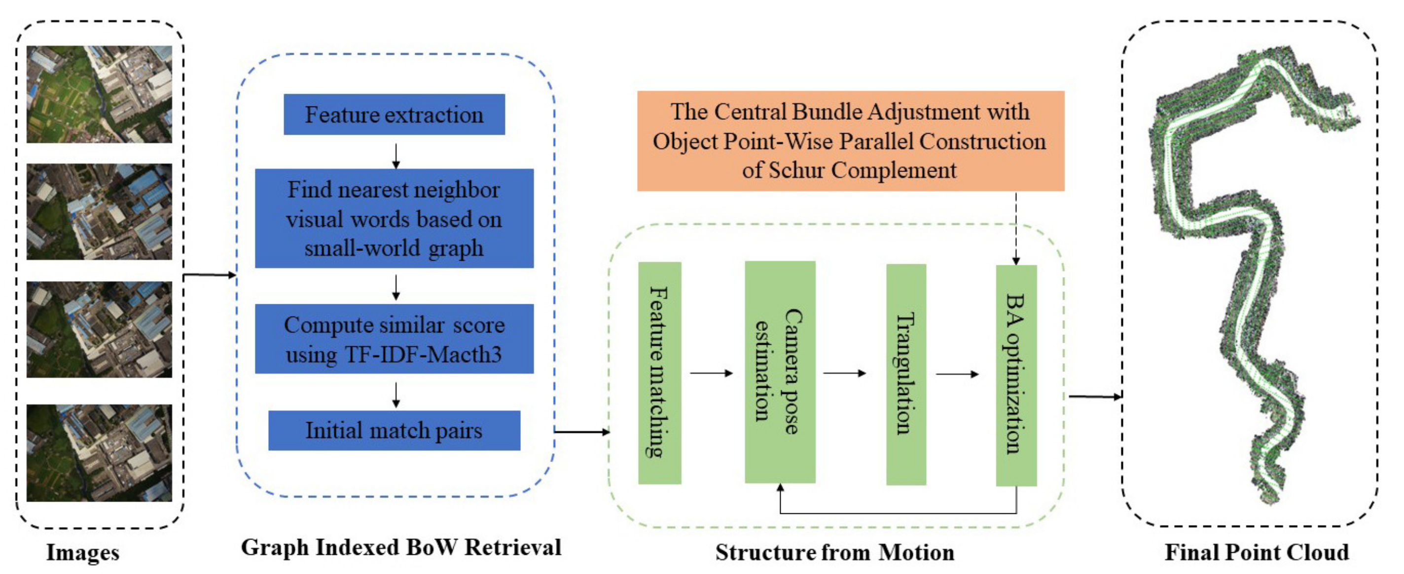
This paper proposes an overall workflow to achieve efficient SfM of large-scale UAV images, as shown in Figure 1. The workflow consists of four main parts: (1) finding UAV image match pairs based on the graph-indexed BoW model; (2) UAV image feature extraction and feature matching; (3) camera pose estimation and triangulation; and (4) central bundle adjustment with object point-wise parallel construction of the Schur complement. Each step in the whole workflow is described as follows:
2.1. Finding UAV Image Match Pairs Based on Graph-Indexed BoW Model
2.1.1. Offline Small-World Graph Structure Construction
In previous studies, using different training datasets to construct words would have an impact on the accuracy and efficiency of image retrieval. Considering this problem, we make certain constraints on the image selection of the training dataset and only select UAV images with a high percentage of urban building parts as the training dataset. In this paper, we use the urban UAV images of Qingdao city in Shandong province as the training data for constructing visual words, which have 83,261 images and cover the area all within the city area, and some sample images are shown in Figure 2. The whole offline construction process is shown in Figure 3.
First, a set of feature descriptors is obtained by extracting local features using images from the training dataset. SIFT is invariant to scale, rotation, illumination, and viewpoint, and it has good perspective distortion tolerance. The SIFTGPU algorithm, which is a gpu-accelerated algorithm for extracting SIFT features with default parameter settings, is used in this paper [46]. The local regions of the feature points are described using 128-dimensional feature vectors, and finally, a training dataset was acquired with 861,709,511 feature descriptors. In order to build the visual word, as Nister showed, the entire set of descriptors is clustered in an iterative way [15], where the maximum number of children per parent node is 512 and the tree structure depth is set to 3; visual words are the leaf nodes of a tree structure. After that, this paper constructs the small-world graph structure of visual words using all visual words as the candidate vertex set V. The main steps include: (1) randomly select a vertex from the set of candidate vertices V; (2) insert the vertex into the graph, and find the f nearest-neighbor vertices to the vertex in the graph, or find the maximum number if there are fewer than f neighboring vertices; (3) build the edge connection relationship between and these neighboring vertices; and (4) repeat steps 1, 2, and 3 until the set of candidate vertices is empty. The detailed construction process is shown in Figure 4. The parameter f is the number of visual words per vertex specified to find the nearest neighbor, which is set to 3 in this paper.
2.1.2. Find Nearest Neighbor Visual Words Based on Small-World Graph Structure
Based on the constructed small-world graph structure of visual words, the feature descriptors of query images can find the corresponding visual words, and thus the query images can be represented by a set of visual words. One of the key steps is how to rapidly find the corresponding visual words, which is the closest Euclidean distance visual word to the descriptor. The proposed nearest-neighbor search algorithm based on the small-world graph structure of visual words is shown in Algorithm 1. The basic idea of the algorithm is as follows: G is initial visual word index, which is stored in priority queue q in descending order of distance, and then the visual word index nearest to the query descriptor is picked up from q (line 2), updating the candidate visual words in the priority queue in descending order of distance (lines 3–9). After that, the f visual word indexes closest to the visual word index in the small-world graph that are inserted into q for the next search (line 10). The visual word index is added to . The search loop (lines 2–17) stops when the distance of the visual word extracted from the priority queue q with descriptor is larger than the distance of the candidate visual word whose distance with descriptor is the largest in (lines 4–5). Figure 5 represents a specific example of the process of finding the nearest visual word based on the graph-indexed structure. The right part displays the state for both priority queues q and , as well as the set for each iteration and the algorithm search path from G → F → C → E.
| Algorithm 1: Finding Nearest Visual Words via Small-World Graph Structure |
 |
The distance calculation between descriptors and visual words is the most time-consuming step. Therefore, this paper implements the distance calculation between descriptors and visual words on the GPU. A warp is used to find the nearest-neighbor visual words of a descriptor. Figure 6 gives an example of the GPU of a warp based on the small-world graph structure nearest-neighbor search word process, mainly divided into 3 steps: (1) obtain the small-world graph index; (2) distance calculation; and (3) data structure maintenance. The details are listed as follows:
- Obtain small-world graph index: We build the small-world graph structure with each vertex fixedly connected to the 3 nearest vertices, occupying a fixed-size space, and store the small-world graph to the GPU. We can locate words by multiplying the fixed-size offset because each word index occupies the same size in memory.
- Distance calculation: Obtain the corresponding visual word from the small-world graph and calculate the distance between the descriptor and the visual word; all threads in a warp are involved in this step. Each thread is responsible for 4 dimensions of a descriptor and calculates the distance between 128-dimensional descriptors and visual words in parallel, and finally, the 1st thread counts the results of all thread calculations and exports the results to an array in shared memory as in Figure 6.
- Data structure maintenance: The query process accesses , q, and and is visited many times, so they are stored in shared memory. Shared memory is a high-speed memory space in each stream processor (SM), and stream processors access it much faster than global memory.
2.1.3. TF–IDF-Match3 Algorithm
The TF–IDF algorithm is used to calculate the similarity between images. Term Frequency (TF) represents the number of occurrences of a visual word in the image, with more occurrences representing the greater importance of the visual word. Inverse Document Frequency (IDF) is a measure of the unique character of a visual word. If a visual word appears in only a few images, the visual word has a high uniqueness. Using the TF–IDF algorithm, the image can be expressed as a BoW vector . Then, the Equation (1) for the component element of BoW vector :
where represents the number of times word i is in indexed image d; represents the total number of visual words contained in indexed image d; is the number of images containing visual word i; N represents the total number of indexed images; and represents the order number of the visual word.
Traditionally, when calculating the score between the query image and the database image, the BoW vector of the image is usually iterated. Additionally, if the same visual words appear, the visual word weights of the query image and the corresponding visual word weights of the database image are multiplied and accumulated to the similarity, as shown in Figure 7. The TF–IDF-Match3 algorithm is proposed in this paper. Before calculating the similarity value between the query image and the database image, assuming that the total number of words is M, the BoW vector of the image is filled to the M dimension. Its weight is assigned to zero for the visual word that does not appear, and the weights of other visual words are kept fixed. In this case, the similarity can be calculated by simply multiplying the BoW vectors in a cycle and then summing them up, as shown in Figure 8. Implementing this computation process on the GPU, a thread is responsible for computing the similarity between the query image and an image in the database, and the following GPU optimization is used to compute the score: (1) The BoW vector of the query image needs to compute the score with all images in the database, and there are frequent accesses. So, the BoW vector of the query image is copied to a shared memory; (2) all threads in the block will access the shared memory at the same time and bank conflict will occur, which allows only one thread to access the bank and the other threads will have to wait. This will significantly reduce the computational efficiency. Therefore, we add one dimension to the query image BoW vector and assign it to zero. After that, multiple threads can access the channels separately, reducing the number of bank conflicts; (3) Using float4 type to store BoW vector, compared with a float type, multibyte vector load or store only need to issue a single instruction; the ratio of bytes per instruction is higher, and the total instruction latency of a particular memory transaction is lower, reducing the number of transaction requests and improving computational efficiency.
2.2. Feature Extraction and Feature Matching
SIFT feature descriptors can effectively cope with lighting and scale changes, rotational transformations, etc. Therefore, this paper uses SiftGPU for feature extraction of UAV images. After that, feature matching needs to be performed. For the two feature descriptors extracted on two images, the Euclidean distance between their corresponding feature vectors can be calculated to evaluate the similarity of these two feature descriptors. In this paper, we adopt the RANSAC-based feature matching method [47] to calculate the homography matrix to describe the transformation relationship of the feature descriptors in two images. The matching error is reduced by continuously updating the matching points and the homography matrix, and finally a homography matrix with minimum matching error and a matching relationship satisfying this homography matrix is calculated, which effectively constrains the distribution of matching feature descriptors and improves the robustness of feature matching.
2.3. The Central Bundle Adjustment with Object Point-Wise Parallel Construction of Schur Complement
2.3.1. LM Algorithm
The function of a bundle adjustment is mainly to solve the unknown vectors of object point, image, and camera that are closest to the true value through continuous update iterations. The image unknown vector is composed of internal orientation elements and external orientation elements. The camera unknown vector consists of focal length, principal point, and distortion parameters. The object point unknown vector is made up of coordinates. It has been shown in many earlier studies [41] that bundle adjustment actually solves the normal equation continuously, and the normal equation is given in Equation (2).
where represents the Jacobian matrix. D is the damping element parameter matrix, which is the diagonal matrix of . is the parameter to adjust the damping element step. Vector is the increment value of unknowns, and is the projection residual vector.
2.3.2. Object Point-Wise Parallel Construction of Schur Complement
In this paper, the internal and external orientation elements of the images, camera parameters, and object points are used as unknown parameters. The Jacobian matrix can also be divided into three categories: , damping matrix , and correction vector . , , and indicate the object point part, image part, and camera part. After that, Equation (3) can be deduced from Equation (2):
Let , , ,
From Equation (4), we know that is a sparse matrix of block stores. and are block matrices with non-sparse store on the diagonal. Because the number of object point unknown vectors is much larger than the total number of image and camera unknown vectors, before solving the unknown vectors, the object point unknowns are first brought into Equation (5) as the known vectors to solve for the image unknowns and camera unknowns . Then, the image and camera unknowns are brought into Equation (6) to solve for the object point unknowns . The matrix is known as the Schur complement. The following expressions for Equations (5) and (6) are given:
According to the above, constructing the Schur complement is the most important part of the bundle adjustment. Because of the separable character of the object points, we propose a central bundle adjustment with object point-wise parallel construction of the Schur complement, which mainly includes the following steps: (1) Apply the memory space for the Schur complement: before performing the bundle adjustment, it is required to iterate through the array of image points corresponding to a single object point. By using the image IDs and camera IDs corresponding to the image points in the image point array, we can know which matrix blocks in the Schur complement need to be filled. In this way, the memory space occupied by the total dataset of the Schur complement can be requested. (2) Calculate the Jacobian matrix and the projected residual matrix for a single object point: calculate the Jacobian matrix for each image point in the array of image points involved in a single object point, that is and . (3) Calculate the normal equation of a single object point: the calculated part of the normal equation block, directly filled into the Schur complement to the diagonal block. (4) Fill in the Schur complement for a single object point: use the block and block part of the normal equation for a single object point, filling in the remaining part. (5) Release the memory occupied by single object points: release the memory of error equation and normal equation of single object points. Steps (2), (3), (4), and (5) are accelerated using CPU multithreading. When a single object point the Schur complement is constructed, the memory occupied by the temporary error equation and the temporary normal equation can be released, greatly reducing memory requirements. Figure 9 represents a specific example of the process of filling in the Schur complement directly at a single object point.
2.3.3. Preconditioned Conjugate Gradient
The most popular method for solving large systems of linear equations is to use CG algorithms for iterative solve. In this paper, the CG method is used to solve the Schur complement. In Equation (5), let , , , then it can be rewritten as Equation (7):
The above process is known as the PCG method. Within this paper, the preprocessing process uses the block diagonal of the Schur complement. During the conjugate gradient iterative solution, the matrix–vector multiplication operation is performed directly using the previously constructed Schur complement, and this computation process is implemented on the GPU. More information on the PCG algorithm can be found in the following articles [48,49,50].
3. Experimental Results
To test the performance of the proposed algorithm, experiments are executed using four datasets of UAV image, as in Table 1. To begin with, we evaluate the performance of the algorithm based on the graph-indexed BoW model to find UAV image match pairs in terms of retrieval accuracy, efficiency, and the number of match pairs and compare its performance with the traditional BoW model retrieval algorithms in Colmap [25] and Dbow2 [26]. Then, after the completed triangulation in SfM, the central bundle adjustment with object point-wise parallel construction of the Schur complement is adopted. In terms of overall memory occupation, efficiency, and accuracy, it is compared with the mainstream Ceres non-linear solver library for central bundle adjustment [51]. The C++ programming language was used to implement all the algorithms in this paper. The algorithms were implemented on a windows platform computer with an Intel Core i7-9900K CPU at 3.6 GHz and a GeForce GTX 1060 graphics card with 6G of graphics cache.
3.1. Datasets
The first dataset covers an industrial area including low-rise cottages and roads, as shown in Figure 10a. One nadir camera and two oblique cameras were used to acquire 1030 images. The camera models are all Sony ILCE-6000, with the oblique camera rotated by 45. The size of this camera is 6000 × 4000. The UAV flight altitude was 347.1 m, and the GSD (ground sampling distance) of the acquired UAV images was about 5.36 cm. In addition, 25 GCPS (ground control points) were measured using the Hi-Target iRTK2 GPS receiver to accurately estimate the absolute orientation, and the flight path map and control point layout is shown in Figure 11a.
The second dataset was collected in a rural area. This area mainly includes some high-level residential buildings and roads, and green vegetation surrounds the residential buildings, as shown in Figure 10b. The UAV platform carried a nadir camera and four oblique cameras for photography, acquiring 5665 images. The camera models are all Sony ILCE-7RM4, with the oblique camera rotated by 45. The size of this camera is 9504 × 6336. The UAV flight altitude was 153.8 m, the GSD of the acquired UAV images was about 1.08 cm, and the flight path map is shown in Figure 11b.
The third dataset was taken on a suburban road. The road is mainly filled with some low cottages and some green vegetation, as shown in Figure 10c. The UAV platform carried a nadir camera and four oblique cameras for photography, acquiring 20,297 images. The camera models are all Sony ILCE-5100, with the oblique camera rotated by 45. The size of this camera is 6000 × 4000. The UAV flight altitude was 153.8 m, and the GSD of the acquired UAV images was about 1.08 cm. The flight path map is shown in Figure 11c.
The fourth dataset was taken in a rural area. The area mainly consists of low-building clusters, agricultural land, and bare land, as shown in Figure 10d. The UAV platform carried a nadir camera and four oblique cameras for photography, acquiring 77,357 images. The camera models are all Sony ILCE-5100, with the oblique camera rotated by 45°. The size of this camera is 6000 × 4000. The UAV flight altitude was 87.1m, and the GSD of the acquired UAV images was about 5.7 cm. The flight path map is shown in Figure 11d.
3.2. The Performance of Finding UAV Image Match Pairs Based on Small-World Index Structure
To obtain reference UAV image match pairs, this paper uses Smart3D commercial software to perform aerial triangulation on each dataset, after which the image match pairs with a number of connected points more than 30 are marked as reference match pairs. Among them, the retrieval accuracy metric uses the ratio of the number of correct images n among the top m images in terms of similarity to the query image to the number of actual reference images m. In this paper, m is set to 30 for all datasets. If the reference images are fewer than 30, the maximum number is taken, and the maximum number of images with the highest similarity is also taken for the query images.
The accuracy of match pair selection and the average number of correct match pairs for a single image is given in Figure 12. To visually represent the query results more obviously, Figure 13 represents the retrieval results of one query image from four datasets using the algorithm of this paper. The input query image is the image with yellow edges. The query image uses the graph index BoW model algorithm to find other images in the dataset that have overlapping areas with it. Therefore, images with green edges represent images in the dataset that have overlapping areas with the query image, which are retrieved images.
From the perspective of the accuracy of match pair selection, the method proposed in this paper has the highest retrieval accuracy in four experimental datas, which reaches 96.5%, 92.41%, 85.74%, and 80.32% for the four datasets, respectively. Colmap-BoW ranks second in retrieval accuracy for the four datasets, and Dbow2 has the lowest retrieval accuracy. From the perspective of the average number of correct match pairs for a single image, the method proposed in this paper has the most average number of correct match pairs in four experimental datas, and the average number of correct match pairs for the retrieval of the four datasets reached 26.21, 28.75, 22.82, and 19.11, respectively. Colmap-BoW ranks second in the average number of correctly match pairs retrieved for the four datasets, with Dbow2 having the lowest average number of correctly match pairs retrieved. It can be concluded that the image features are more accurate in searching for the corresponding visual words using the graph structure, and therefore the BoW vector expression of the image is more accurate. So, the average number of correct match pairs and the retrieval accuracy are higher.
Table 2 gives detailed information on the time taken to search for visual words and calculate scores during match pairs retrieval. From the perspective of the efficiency of finding the nearest visual word, the method of finding nearest-neighbor visual words based on small-world graph structure has the highest retrieval efficiencies in the four experimental datasets, which reach 0.82 min, 14.05 min, 98.69 min, and 568.74 min for the four datasets, respectively. Colmap-BoW and Dbow2 are approximately equally efficient on the four datasets. This shows that finding nearest-neighbor visual words based on the small-world graph structure of visual word is more efficient than K-Means search. From the perspective of calculating the image similarity score, the TF–IDF-Match3 algorithm proposed in this paper has the highest calculating efficiencies in the four experimental datasets, which reach 0.167 min, 1.044 min, 5.73 min, and 17.024 min for the four datasets, respectively. Dbow2 ranks second in the efficiency of calculating scores for the four datasets. On dataset 3 and dataset 4, Colmap-Bow took more than 24 h, so the calculation efficiency is only compared with dataset 1 and dataset 2, both of which were the lowest. It can be concluded that the TF–IDF-Match3 algorithm can effectively improve calculation efficiency.
Figure 14 gives the relative ratio of the overall time consumption of the three algorithms on the four experimental datasets. From the perspective of overall time consumption, the proposed algorithm in this paper has the highest efficiency. On Dataset 1, the proposed algorithm is 7.3 times and 15.6 times more efficient than Dbow2 and Colmap-Bow; on Dataset 2, the proposed algorithm is 4.3 and 13.9 times more efficient than Dbow2 and Colmap-Bow. On Datasets 3 and 4, Colmap-Bow took more than 24 h, which is not meaningful for comparison and belongs to the invalid dataset. So, the proposed algorithm is only compared with Dbow2, which improves 3.9 times and 3.8 times on dataset 3 and dataset 4, respectively. It can be seen that the proposed algorithm improves the computation efficiency by 3–7 times on the effective datasets.
3.3. The Performance of Central Bundle Adjustment with Object Point-Wise Parallel Construction of Schur Complement
In this paper, the framework of the LM algorithm is combined with PCG to iteratively solve the Schur complement. Among them, the upper limits of the number of iterations of the LM algorithm are set to 20, and the upper limits of the number of iterations of the PCG operation are set to 300.
Figure 15 shows the relative ratio of peak memory occupation and the relative ratio of efficiency for the two bundle adjustment algorithms on the four experimental datasets. From the perspective of peak memory occupation, it can be shown in Table 3 that the proposed algorithm has a peak memory occupation of 556.7 MB, while the Ceres algorithm has a peak occupation of 1263.3 MB on dataset 1, with a significantly lower peak memory requirement. Moreover, it can be shown in Figure 15 that the proposed algorithm reduces by 2.27 times the peak memory occupation compared with the Ceres algorithm on dataset 1. On dataset 2, the proposed algorithm occupies a peak memory of 1756.1MB, and Ceres occupies a peak memory of 4151.7 MB, which reduces 2.36 times. On dataset 3, the proposed algorithm occupies a peak memory of 10,504.2MB, and Ceres occupies a peak memory of 29,727.6 MB, which reduces 2.83 times. On dataset 4, the proposed algorithm occupies a peak memory of 17,221.8 MB, and Ceres occupies a peak memory of 49,786.8 MB, which reduces 2.89 times. It can be clearly inferred that as the number of data increases, the more significantly the memory occupation is reduced, and the proposed algorithm reduces the memory occupation peak by 2–3 times compared with Ceres. From the perspective of the computation efficiency, it can be shown in Table 3 that the proposed algorithm takes 18.141 s overall, while the Ceres algorithm takes 54.655 s overall on dataset 1, with a substantial increase in efficiency. Moreover, it can be shown in Figure 15 that the proposed algorithm has 3.01 times higher efficiency than the Ceres algorithm. On dataset 2, the proposed algorithm took 47.129 s overall, and Ceres took 195.12 s overall, which is an improvement of 4.14 times. On dataset 3, the proposed algorithm took 179.21 s overall, and Ceres took 812.4 MB overall, which is an improvement of 4.53 times. On dataset 4, the proposed algorithm took 639.82 s overall, and Ceres took 4023.66 s overall, which is an improvement of 6.29 times. It can be clearly inferred that the proposed algorithm improves the efficiency by 2–7 times compared with Ceres. From the perspective of the average projection residual of image points after bundle adjustment, the algorithm proposed in this paper and the Ceres algorithm can achieve the same accuracy and efficiency and meet the bundle adjustment requirements.
To evaluate the accuracy of the geo-referenced model after bundle adjustment, ground control points are used to assist the experimental process. There are two types of ground control points in this paper, one is called CPS(control points), and its function is to convert the reference coordinate system of the model to the world coordinate system, this process is called absolute orientation. The other one is called check point, and its role is to check the accuracy of the dataset bundle adjustment results. In this experiment, 25 ground control points were measured in dataset 1. The control points numbered 2, 5, 6, 7, and 10 are used as control points to assist in absolute orientation, which restores the entire scene and converts to a geo-referenced coordinate system. The remaining control points are used as check points. The image points in the bundle adjustment dataset are used for forward intersection, and the coordinates of the intersected object points are compared with the coordinates of the check points, and this residual value is used to evaluate the accuracy of the bundle adjustment results. In this paper, the residual results are analyzed and evaluated in terms of minimum, maximum, mean, and root mean square errors (RMSEs). Table 4 presents the dataset 1 results for the minimum, maximum, and absolute mean values in the X, Y, and Z directions. It can be shown that in the algorithm of this paper, the maximum, minimum, and average values in the X, Y, and Z directions are the same as the Ceres algorithm, and the overall average value in the Z direction of this paper is more accurate than the Ceres algorithm. Figure 16 shows the residual RMSEs in the X, Y, and Z directions. It can be seen that in the algorithm in this paper and the Ceres algorithm, the projected residuals in X, Y, and Z directions are the same, and the residual plots show almost the same trend. To visually represent the bundle adjustment results more obviously, Figure 17 represents the results of using the algorithm of this paper from four datasets. The image on the left is the coordinates measured by the model, and on the right are the coordinates of the ground control points measured outdoors, and it can be shown that the two results are essentially the same. The experimental results for the other three experimental datasets are similar to dataset 1. Additionally, the results of the proposed algorithm and Ceres are the same and meet the bundle adjustment requirements, so they are not described too much in the paper. Thus, we can draw the conclusion that the algorithm of this paper is fully accurate to meet the requirements of bundle adjustment.
4. Discussion
In this paper, an efficient solution for large-scale UAV image SfM is proposed to solve the problems of the high memory consumption and low efficiency of large-scale UAV image SfM. It consists of two main aspects, including the selection of UAV image match pairs based on the graph-indexed BoW model and a central bundle adjustment with object point-wise parallel construction of the Schur complement algorithm. The results show that the proposed method is an efficient and low memory consumption SfM solution for large-scale UAV images, and the image points cloud results are shown in Figure 18. Two sides of its performance can be considered.
To begin with, using the graph index BoW model algorithm can find match pairs of UAV images with overlapping regions, which can provide reliable match pairs for feature matching and significantly improve the efficiency of feature matching. This can be explained in two aspects. On the one hand, it avoids exhaustive listing of all image match pairs, effectively removes the match pairs without overlapping regions, and reduces the total number of match pairs to be feature matched. On the other hand, those match pairs with small or narrow overlapping areas are effectively removed, reducing the number of false matches. Effective match pair selection can effectively solve this problem. For the four experimental datasets, compared with Colmap-Bow and Dbow2, the acceleration ratio of this paper’s method to select match pairs reaches 3–7 times, as shown in Figure 14. To compare the accuracy issue, we can see that the match pair retrieval accuracies of the method in this paper are the highest, as shown in Figure 12.
Then, the central bundle adjustment with object point-wise parallel construction of the Schur complement algorithm can not only improve efficiency but also reduce the overall memory occupation requirement compared with Ceres’ non-linear solution library for solving. On the one hand, the overall memory requirement is reduced by constructing a temporary error equation and temporary normal equation for the object points, and then releasing the temporary memory after filling in the Schur complement. On the other hand, during the conjugate gradient iterative solution process, the process of construction of the Schur complement using the error equation for each iteration is eliminated, and the previously constructed Schur complement is used instead, which can significantly improve the overall efficiency. The speed-up ratio of this method reaches 2–7 times with four experimental datasets, and the memory occupation is reduced by 2–3 times, as shown in Figure 15. Additionally, the same accuracy can be achieved with Ceres.
5. Conclusions
In this paper, we propose an efficient SfM solution for large-scale UAV images, which finds image match pairs based on the graph-indexed BoW model and executes BA optimization with object point-wise parallel construction of the Schur complement. The graph index BoW model algorithm is used to search for UAV image match pairs which do not rely on location parameter information and do not require exhaustive computation. The central bundle adjustment with object point-wise parallel construction of the Schur complement algorithm improves the efficiency of the traditional bundle adjustment and significantly reduces memory consumption. Finally, by comprehensively analyzing and comparing four UAV datasets captured using different oblique multicamera systems to evaluate the proposed SfM solution, the experimental results show that the graph index BoW model can efficiently and accurately select match pairs with overlapping areas, and the central bundle adjustment with object point-wise parallel construction of the Schur complement algorithm can efficiently and accurately obtain the bundle adjustment result. The method proposed in this paper is an efficient solution for the SfM of large-scale UAV images.
Although the proposed graph index BoW model algorithm is advantageous in terms of efficiency, there is the problem of losing some real match pairs in feature matching. As shown in Figure 12, the accuracy of match pairs tends to decrease as the amount of data increases. This problem can be explained by the pretrained vocabulary tree. On the one hand, the increase in data volume leads to more kinds of image features, but the pretrained vocabulary tree model does not cover all kinds of image features. So, the image features may find the wrong visual words, which reduces retrieval accuracy. On the other hand, the depth and number of branches of the pretrained vocabulary tree determine the total number of clustered visual words, and as the data volume increases, different image features may find the same visual words, which reduces the retrieval accuracy. Therefore, future research can focus on the types of pretrained images and the size of the vocabulary tree to improve match pair accuracy further.
Author Contributions
B.G. and S.L. validated and implement the experiments; S.L. wrote and tested the experiments; S.J. and Y.L. and W.X. investigated and counted the results; S.L. wrote and edited the paper. All authors have read and agreed to the published version of the manuscript.
Funding
The National Natural Science Foundation of China (Grant No. 42001413).
Acknowledgments
Thanks to the authors who created the SiftGPU, Colmap, and Dbow2 algorithms and made them open source. These algorithms were very valuable for this study. Thanks to Wuhan University Huawei Geoinformatics Innovation Labpratory.
Conflicts of Interest
The authors declare no conflict of interest.
References
- Lin, Y.; Jiang, M.; Yao, Y.; Zhang, L.; Lin, J. Use of UAV oblique imaging for the detection of individual trees in residential environments. Urban For. Urban Green. 2015, 14, 404–412. [Google Scholar] [CrossRef]
- Jiang, S.; Jiang, W.; Huang, W.; Yang, L. UAV-based oblique photogrammetry for outdoor data acquisition and offsite visual inspection of transmission line. Remote Sens. 2017, 9, 278. [Google Scholar] [CrossRef] [Green Version]
- Aicardi, I.; Chiabrando, F.; Grasso, N.; Lingua, A.M.; Noardo, F.; Spanò, A. UAV Photogrammetry with Oblique Images: First Analysis on Data Acquisition and Processing. Int. Arch. Photogramm. Remote Sens. Spat. Inf. Sci. 2016, 41, 835–842. [Google Scholar] [CrossRef] [Green Version]
- Jiang, S.; Jiang, C.; Jiang, W. Efficient structure from motion for large-scale UAV images: A review and a comparison of SfM tools. ISPRS J. Photogramm. Remote Sens. 2020, 167, 230–251. [Google Scholar] [CrossRef]
- Westoby, M.J.; Brasington, J.; Glasser, N.F.; Hambrey, M.J.; Reynolds, J.M. ‘Structure-from-Motion’photogrammetry: A low-cost, effective tool for geoscience applications. Geomorphology 2012, 179, 300–314. [Google Scholar] [CrossRef] [Green Version]
- Snavely, N.; Seitz, S.M.; Szeliski, R. Photo tourism: Exploring photo collections in 3D. In ACM Siggraph 2006 Papers; Association for Computing Machinery: New York, NY, USA, 2006; pp. 835–846. [Google Scholar]
- Caroti, G.; Martinez Espejo Zaragoza, I.; Piemonte, A. Accuracy assessment in structure from motion 3D reconstruction from UAV-born images: The influence of the data processing methods. Int. Arch. Photogramm. Remote Sens. Spat. Inf. Sci. 2015, XL-1/W4, 103–109. [Google Scholar] [CrossRef] [Green Version]
- Zhang, R.; Schneider, D.; Strauß, B. Generation and comparison of TLS and SFM based 3d models of solid shapes in hydromechanic research. Int. Arch. Photogramm. Remote Sens. Spat. Inf. Sci. 2016, 41, 925. [Google Scholar] [CrossRef] [Green Version]
- Ippoliti, E.; Meschini, A.; Sicuranza, F. Structure from motion systems for architectural heritage. A survey of the internal logGia Court. Palazzo Dei Capitani, Ascoli Piceno, Italy. Int. Arch. Photogramm. Remote Sens. Spat. Inf. Sci. 2015, 40, 53. [Google Scholar] [CrossRef] [Green Version]
- Tonkin, T.N.; Midgley, N.G.; Graham, D.J.; Labadz, J. The potential of small unmanned aircraft systems and structure-from-motion for topographic surveys: A test of emerging integrated approaches at Cwm Idwal, North Wales. Geomorphology 2014, 226, 35–43. [Google Scholar] [CrossRef] [Green Version]
- Cao, M.; Li, S.; Jia, W.; Li, S.; Liu, X. Robust bundle adjustment for large-scale structure from motion. Multimed. Tools Appl. 2017, 76, 21843–21867. [Google Scholar] [CrossRef]
- Zheng, M.; Zhang, F.; Zhu, J.; Zuo, Z. A fast and accurate bundle adjustment method for very large-scale data. Comput. Geosci. 2020, 142, 104539. [Google Scholar] [CrossRef]
- Shen, T.; Zhu, S.; Fang, T.; Zhang, R.; Quan, L. Graph-based consistent matching for structure-from-motion. In Proceedings of the European Conference on Computer Vision, Springer, Amsterdam, The Netherlands, 8–16 October 2016; pp. 139–155. [Google Scholar]
- Jiang, S.; Jiang, W.; Guo, B. Leveraging vocabulary tree for simultaneous match pair selection and guided feature matching of UAV images. ISPRS J. Photogramm. Remote Sens. 2022, 187, 273–293. [Google Scholar] [CrossRef]
- Nister, D.; Stewenius, H. Scalable recognition with a vocabulary tree. In Proceedings of the 2006 IEEE Computer Society Conference on Computer Vision and Pattern Recognition (CVPR’06), IEEE, New York, NY, USA, 17–22 June 2006; Volume 2, pp. 2161–2168. [Google Scholar]
- Jiang, S.; Jiang, W. Efficient structure from motion for oblique UAV images based on maximal spanning tree expansion. ISPRS J. Photogramm. Remote Sens. 2017, 132, 140–161. [Google Scholar] [CrossRef]
- Datta, R.; Joshi, D.; Li, J.; Wang, J.Z. Image retrieval: Ideas, influences, and trends of the new age. ACM Comput. Surv. (Csur) 2008, 40, 1–60. [Google Scholar] [CrossRef]
- Halawani, A.; Teynor, A.; Setia, L.; Brunner, G.; Burkhardt, H. Fundamentals and Applications of Image Retrieval: An Overview. Datenbank-Spektrum 2006, 18, 6. [Google Scholar]
- Sivic, J.; Zisserman, A. Video Google: A text retrieval approach to object matching in videos. In Proceedings of the Computer Vision, IEEE International Conference on, IEEE Computer Society, Tunis, Tunisia, 14–18 July 2003; Volume 3, p. 1470. [Google Scholar]
- Radenović, F.; Tolias, G.; Chum, O. CNN image retrieval learns from BoW: Unsupervised fine-tuning with hard examples. In Proceedings of the European Conference on Computer Vision, Springer, Amsterdam, The Netherlands, 8–16 October 2016; pp. 3–20. [Google Scholar]
- Rupnik, E.; Nex, F.; Remondino, F. Automatic orientation of large blocks of oblique images. In Proceedings of the International Archives of the Photogrammetry, Remote Sensing and Spatial Information Science, ISPRS HannoverWorkshop 2013, Hannover, Germany, 21–24 May 2013. [Google Scholar]
- Lowe, D.G. Distinctive image features from scale-invariant keypoints. Int. J. Comput. Vis. 2004, 60, 91–110. [Google Scholar] [CrossRef]
- Arai, K.; Ridho, A. Hierarchical K-Means: An Algorithm for Centroids Initialization for K-Means; Saga University: Saga, Japan, 2007. [Google Scholar]
- Sivic, J.; Zisserman, A. Efficient visual search of videos cast as text retrieval. IEEE Trans. Pattern Anal. Mach. Intell. 2008, 31, 591–606. [Google Scholar] [CrossRef] [Green Version]
- Schonberger, J.L.; Frahm, J.M. Structure-from-motion revisited. In Proceedings of the IEEE Conference on Computer Vision and Pattern Recognition, Las Vegas, NV, USA, 27–30 June 2016; pp. 4104–4113. [Google Scholar]
- Gálvez-López, D.; Tardos, J.D. Bags of binary words for fast place recognition in image sequences. IEEE Trans. Robot. 2012, 28, 1188–1197. [Google Scholar] [CrossRef]
- Gionis, A.; Indyk, P.; Motwani, R. Similarity search in high dimensions via hashing. In Proceedings of the Vldb, Edinburgh, UK, 7–10 September 1999; Volume 99, pp. 518–529. [Google Scholar]
- Weiss, Y.; Fergus, R.; Torralba, A. Multidimensional spectral hashing. In Proceedings of the European Conference on Computer Vision, Springer, Florence, Italy, 7–13 October 2012; pp. 340–353. [Google Scholar]
- Cayton, L. Fast nearest neighbor retrieval for bregman divergences. In Proceedings of the 25th International Conference on Machine Learning, Helsinki, Finland, 5–9 July 2008; pp. 112–119. [Google Scholar]
- Finkel, R.A.; Bentley, J.L. Quad trees a data structure for retrieval on composite keys. Acta Inform. 1974, 4, 1–9. [Google Scholar] [CrossRef]
- Curtin, R.R.; Ram, P.; Gray, A.G. Fast exact max-kernel search. In Proceedings of the 2013 SIAM International Conference on Data Mining, SIAM, Austin, TX, USA, 2–4 May 2013; pp. 1–9. [Google Scholar]
- Malkov, Y.A.; Yashunin, D.A. Efficient and robust approximate nearest neighbor search using hierarchical navigable small world graphs. IEEE Trans. Pattern Anal. Mach. Intell. 2018, 42, 824–836. [Google Scholar] [CrossRef] [Green Version]
- Fu, C.; Xiang, C.; Wang, C.; Cai, D. Fast approximate nearest neighbor search with the navigating spreading-out graph. arXiv 2017, arXiv:1707.00143. [Google Scholar] [CrossRef]
- Malkov, Y.; Ponomarenko, A.; Logvinov, A.; Krylov, V. Approximate nearest neighbor algorithm based on navigable small world graphs. Inf. Syst. 2014, 45, 61–68. [Google Scholar] [CrossRef]
- Nickolls, J.; Dally, W.J. The GPU computing era. IEEE Micro 2010, 30, 56–69. [Google Scholar] [CrossRef]
- Gou, C.; Gaydadjiev, G.N. Elastic pipeline: Addressing GPU on-chip shared memory bank conflicts. In Proceedings of the 8th ACM International Conference on Computing Frontiers, Ischia, Italy, 3–5 May 2011; pp. 1–11. [Google Scholar]
- Triggs, B.; McLauchlan, P.F.; Hartley, R.I.; Fitzgibbon, A.W. Bundle adjustment—A modern synthesis. In Proceedings of the International Workshop on Vision Algorithms, Springer, Heraklion, Greece, 21–22 September 1999; pp. 298–372. [Google Scholar]
- Eriksson, A.; Bastian, J.; Chin, T.J.; Isaksson, M. A consensus-based framework for distributed bundle adjustment. In Proceedings of the IEEE Conference on Computer Vision and Pattern Recognition, Las Vegas, NV, USA, 27–30 June 2016; pp. 1754–1762. [Google Scholar]
- Zhang, F. The Schur Complement and Its Applications; Springer Science & Business Media: Berlin, Germany, 2006; Volume 4. [Google Scholar]
- Zhang, R.; Zhu, S.; Fang, T.; Quan, L. Distributed very large scale bundle adjustment by global camera consensus. In Proceedings of the IEEE International Conference on Computer Vision, Venice, Italy, 22–29 October 2017; pp. 29–38. [Google Scholar]
- Levenberg, K. A method for the solution of certain non-linear problems in least squares. Q. Appl. Math. 1944, 2, 164–168. [Google Scholar] [CrossRef] [Green Version]
- Dellaert, F.; Carlson, J.; Ila, V.; Ni, K.; Thorpe, C.E. Subgraph-preconditioned conjugate gradients for large scale SLAM. In Proceedings of the 2010 IEEE/RSJ International Conference on Intelligent Robots and Systems, IEEE, Taipei, Taiwan, 18–22 October 2010; pp. 2566–2571. [Google Scholar]
- Liu, Q.; Li, X. Preconditioned conjugate gradient methods for the solution of indefinite least squares problems. Calcolo 2011, 48, 261–271. [Google Scholar] [CrossRef]
- Ye, Z.; Li, G.; Liu, H.; Cui, Z.; Bao, H.; Zhang, G. CoLi-BA: Compact Linearization based Solver for Bundle Adjustment. IEEE Trans. Vis. Comput. Graph. 2022, 28, 3727–3736. [Google Scholar] [CrossRef]
- Alismail, H.; Browning, B.; Lucey, S. Photometric bundle adjustment for vision-based slam. In Proceedings of the Asian Conference on Computer Vision, Springer, Taipei, Taiwan, 20–24 November 2016; pp. 324–341. [Google Scholar]
- Wu, C. A GPU Implementation of Scale Invariant Feature Transform (SIFT). 2017. Available online: https://cir.nii.ac.jp/crid/1573105976089193856 (accessed on 15 March 2022).
- Fischler, M.A.; Bolles, R.C. Random sample consensus: A paradigm for model fitting with applications to image analysis and automated cartography. Commun. ACM 1981, 24, 381–395. [Google Scholar] [CrossRef]
- Zheng, M.; Zhang, Y.; Zhou, S.; Zhu, J.; Xiong, X. Bundle block adjustment of large-scale remote sensing data with Block-based Sparse Matrix Compression combined with Preconditioned Conjugate Gradient. Comput. Geosci. 2016, 92, 70–78. [Google Scholar] [CrossRef]
- Agarwal, S.; Snavely, N.; Seitz, S.M.; Szeliski, R. Bundle adjustment in the large. In Proceedings of the European Conference on Computer Vision, Springer, Heraklion, Greece, 5–11 September 2010; pp. 29–42. [Google Scholar]
- Wu, C.; Agarwal, S.; Curless, B.; Seitz, S.M. Multicore bundle adjustment. In Proceedings of the CVPR 2011, IEEE, Washington, DC, USA, 20–25 June 2011; pp. 3057–3064. [Google Scholar]
- Agarwal, S.; Mierle, K. Ceres Solver. 2012. Available online: https://github.com/ceres-solver/ceres-solver (accessed on 15 March 2022).
Figure 1.
The workflow of the proposed SfM solution.

Figure 2.
UAV image training data collection in Qingdao, Shandong province.

Figure 3.
The workflow of the offline small-world graph structure of visual word construction.

Figure 4.
Small-world graph structure of visual word construction process.

Figure 5.
Specific example of the nearest-neighbor search based on the small-world graph structure of visual words.
Figure 5.
Specific example of the nearest-neighbor search based on the small-world graph structure of visual words.

Figure 6.
Nearest word search process on the GPU.

Figure 7.
TF–IDF similarity calculation method.

Figure 8.
TF–IDF-Match3 similarity calculation method.

Figure 9.
Single object points directly fill in the Schur complement.


Figure 10.
Four datasets of UAV experiments. (a) Dataset 1. (b) Dataset 2. (c) Dataset 3. (d) Dataset 4.
Figure 10.
Four datasets of UAV experiments. (a) Dataset 1. (b) Dataset 2. (c) Dataset 3. (d) Dataset 4.

Figure 11.
Flight path map of the experimental dataset. (a) Dataset 1. (b) Dataset 2. (c) Dataset 3. (d) Dataset 4.
Figure 11.
Flight path map of the experimental dataset. (a) Dataset 1. (b) Dataset 2. (c) Dataset 3. (d) Dataset 4.

Figure 12.
Match pair retrieval accuracy and average number of correct match pairs for a single image. (a) Retrieval accuracy. (b) Average number of correct match pairs.
Figure 12.
Match pair retrieval accuracy and average number of correct match pairs for a single image. (a) Retrieval accuracy. (b) Average number of correct match pairs.

Figure 13.
Example of retrieval result from four datasets. (a) Dataset 1. (b) Dataset 2. (c) Dataset 3. (d) Dataset 4.
Figure 13.
Example of retrieval result from four datasets. (a) Dataset 1. (b) Dataset 2. (c) Dataset 3. (d) Dataset 4.

Figure 14.
Overall retrieval efficiency relative ratio.

Figure 15.
Bundle adjustment efficiency and memory relative ratio. (a) BA efficiency relative ratio. (b) BA memory occupation relative ratio.
Figure 15.
Bundle adjustment efficiency and memory relative ratio. (a) BA efficiency relative ratio. (b) BA memory occupation relative ratio.

Figure 16.
Each residual plot in the X, Y, and Z directions for dataset 1: (a) the residual plot in the X direction; (b) the residual plot in the Y direction; (c) the residual plot in the Z direction.
Figure 16.
Each residual plot in the X, Y, and Z directions for dataset 1: (a) the residual plot in the X direction; (b) the residual plot in the Y direction; (c) the residual plot in the Z direction.

Figure 17.
A sample of control points from four datasets. In each subplot, the left side is measured model coordinates, and the right side is outdoor ground control point coordinates. (a) Dataset 1. (b) Dataset 2. (c) Dataset 3. (d) Dataset 4.
Figure 17.
A sample of control points from four datasets. In each subplot, the left side is measured model coordinates, and the right side is outdoor ground control point coordinates. (a) Dataset 1. (b) Dataset 2. (c) Dataset 3. (d) Dataset 4.

Figure 18.
Image points cloud of the experimental dataset. (a) Dataset 1. (b) Dataset 2. (c) Dataset 3. (d) Dataset 4.
Figure 18.
Image points cloud of the experimental dataset. (a) Dataset 1. (b) Dataset 2. (c) Dataset 3. (d) Dataset 4.


Table 1.
Details of the experimental dataset.
| Item Name | Dataset 1 | Dataset 2 | Dataset 3 | Dataset 4 |
|---|---|---|---|---|
| UAV type | Multirotor | Multirotor | Multirotor | Multirotor |
| Flight height (m) | 347.1 | 153.8 | 192.9 | 87.1 |
| Camera mode | ILCE-6000 | ILCE-7RM4 | ILCE-5100 | ILCE-5100 |
| Number of cameras | 3 | 5 | 5 | 5 |
| Focal length (mm) | 25 | 56 | 35 | 35 |
| Camera mount angle (degree) | nadir:0 oblique: −45∖45 | nadir:0 oblique: −45∖45 | nadir:0 oblique: −45∖45 | nadir:0 oblique: −45∖45 |
| Number of images | 1030 | 5665 | 20,297 | 77,357 |
| Image size (pixel × pixel) | 6000 × 4000 | 9504 × 6336 | 6000 × 4000 | 6000 × 4000 |
| GSD (cm) | 5.36 | 1.08 | 5.7 | 1.21 |
| Image point number | 885,822 | 3,079,359 | 24,371,628 | 40,835,177 |
| Object point number | 209,624 | 736,774 | 3,869,464 | 6,534,761 |
Table 2.
Match pair retrieval specific time consumption.
| Metric | Method | Dataset 1 | Dataset 2 | Dataset 3 | Dataset 4 |
|---|---|---|---|---|---|
| Retrieval word efficiency (min) | Colmap-BoW | 2.5108 | 29.729 | 204.15 | 1052.04 |
| Dbow2 | 2.3689 | 29.404 | 201.92 | 1048.66 | |
| GIBoW | 0.8232 | 14.054 | 98.69 | 568.74 | |
| Compute image score efficiency (min) | Colmap-BoW | 12.1224 | 177.27175 | NULL | NULL |
| Dbow2 | 4.21 | 35.93 | 205.77 | 1125.70 | |
| GIBoW | 0.167 | 1.044 | 5.73 | 17.024 | |
| overall retrieval time (min) | Colmap-BoW | 15.4832 | 215.75 | NULL | NULL |
| Dbow2 | 7.2789 | 66.335 | 412.69 | 2212.36 | |
| GIBoW | 0.9912 | 15.489 | 105.24 | 589.762 |
Table 3.
Bundle adjustment details metric.
| Metric | Method | Dataset 1 | Dataset 2 | Dataset 3 | Dataset 4 |
|---|---|---|---|---|---|
| Peak Occupied Memory (MB) | Ceres | 1263.3 | 4151.7 | 29727.6 | 49786.8 |
| PSCBA | 556.7 | 1756.1 | 10,504.2 | 17,221.8 | |
| Efficiency (s) | Ceres | 54.655 | 195.12 | 812.4 | 4023.66 |
| PSCBA | 18.141 | 47.129 | 179.21 | 639.82 | |
| Total Average Residua Value (m) | Ceres | 0.030894 | 0.045496 | 0.041592 | 0.056102 |
| PSCBA | 0.026834 | 0.045495 | 0.041272 | 0.056001 |
Table 4.
Metric of ground control points after bundle adjustment for dataset 1.
| Method | Min (m) | Max (m) | Mean (m) | ||||||
|---|---|---|---|---|---|---|---|---|---|
| X | Y | Z | X | Y | Z | X | Y | Z | |
| Ceres | −0.016 | −0.015 | −0.052 | 0.0183 | 0.0121 | 0.0515 | 0.002 | 0.0027 | 0.0070 |
| PSCBA | −0.016 | −0.0123 | −0.0523 | 0.0183 | 0.0122 | 0.0514 | 0.002 | 0.0027 | 0.0068 |
Publisher’s Note: MDPI stays neutral with regard to jurisdictional claims in published maps and institutional affiliations. |
© 2022 by the authors. Licensee MDPI, Basel, Switzerland. This article is an open access article distributed under the terms and conditions of the Creative Commons Attribution (CC BY) license (https://creativecommons.org/licenses/by/4.0/).
Share and Cite
MDPI and ACS Style
Liu, S.; Jiang, S.; Liu, Y.; Xue, W.; Guo, B. Efficient SfM for Large-Scale UAV Images Based on Graph-Indexed BoW and Parallel-Constructed BA Optimization. Remote Sens. 2022, 14, 5619. https://doi.org/10.3390/rs14215619
AMA Style
Liu S, Jiang S, Liu Y, Xue W, Guo B. Efficient SfM for Large-Scale UAV Images Based on Graph-Indexed BoW and Parallel-Constructed BA Optimization. Remote Sensing. 2022; 14(21):5619. https://doi.org/10.3390/rs14215619
Chicago/Turabian StyleLiu, Sikang, San Jiang, Yawen Liu, Wanchang Xue, and Bingxuan Guo. 2022. "Efficient SfM for Large-Scale UAV Images Based on Graph-Indexed BoW and Parallel-Constructed BA Optimization" Remote Sensing 14, no. 21: 5619. https://doi.org/10.3390/rs14215619
Note that from the first issue of 2016, this journal uses article numbers instead of page numbers. See further details here.