
Adaptive Multi-Proxy for Remote Sensing Image Retrieval

1
College of Information Technology, Shanghai Ocean University, Shanghai 201306, China
2
Engineering Training Centre, Shanghai University, Shanghai 200444, China
*
Author to whom correspondence should be addressed.
Remote Sens. 2022, 14(21), 5615; https://doi.org/10.3390/rs14215615
Submission received: 2 August 2022
/
Revised: 24 October 2022
/
Accepted: 1 November 2022
/
Published: 7 November 2022
(This article belongs to the Section Remote Sensing Image Processing)
Abstract
:With the development of remote sensing technology, content-based remote sensing image retrieval has become a research hotspot. Remote sensing image datasets not only contain rich location, semantic and scale information but also have large intra-class differences. Therefore, the key to improving the performance of remote sensing image retrieval is to make full use of the limited sample information to extract more comprehensive class features. In this paper, we propose a proxy-based deep metric learning method and an adaptive multi-proxy framework. First, we propose an intra-cluster sample synthesis strategy with a random factor, which uses the limited samples in batch to synthesize more samples to enhance the network’s learning of unobvious features in the class. Second, we propose an adaptive proxy assignment method to assign multiple proxies according to the cluster of samples within a class, and to determine weights for each proxy according to the cluster scale to accurately and comprehensively measure the sample-class similarity. Finally, we incorporate a rigorous evaluation metric mAP@R and a variety of dataset partitioning methods, and conduct extensive experiments on commonly used remote sensing image datasets.
1. Introduction
In recent years, with the rapid development of remote sensing (RS) technology, the number of remote sensing images has proliferated, and the demand for remote sensing image processing has also increased. Remote sensing images contain a large amount of temporal and spatial data, and play a key role in land management [1,2], urban planning [3,4], environmental protection [5,6], and other fields. Nowadays, the research on remote sensing images has received a lot of attention, such as image classification [7,8,9], image retrieval [10,11,12], feature segmentation [13,14,15], target detection [16,17,18], etc. Among many remote sensing image processing techniques, remote sensing image retrieval (RSIR) technology has been key research. How to retrieve the target sample efficiently and accurately from the huge amount of images is the key point of RSIR technology. Nowadays, RSIR technology has been transformed from the traditional text-based retrieval method to the content-based retrieval method. The content-based RSIR method uses color, texture, and spatial information features to describe the image and achieve higher retrieval performance.
Remote sensing images always contain rich information on geographic location, variable scales, and semantic objects, so the extraction of remote sensing image features is the main challenge for RSIR techniques. Most of the current studies use deep neural networks to extract features of RS images [19,20]. However, in the practical application of deep learning methods, data collection and annotation often consume a lot of time and labor costs. From the perspective of RS images, there are a variety of landscape features all over the world, and it is difficult to produce large-scale and multi-class RS image datasets. Therefore, to cope with massive data retrieval tasks, strong retrieval performances of limited annotated data are important.
Deep metric learning can use a deep neural network to extract sample features, i.e., to obtain the feature vectors of images. Moreover, use the features to calculate the similarity between samples to perform image retrieval tasks. This feature-independent learning method allows metric learning to still have a strong generalization ability on invisible classes (classes that the model has not been trained on). Such methods can greatly reduce the cost of data collection and annotation. Currently, deep metric learning has been widely used in popular computer vision fields such as image classification [21,22], retrieval [23,24], few-shot learning [25,26], and cross-modal retrieval [27,28].
Specifically, deep metric learning aims to train the network to fit a reasonable embedding space and effectively measure the similarity between samples. Current metric learning methods are mainly divided into two types: pair-based [29,30,31] and proxy-based [32,33,34] methods. Pair-based deep metric learning methods compose samples into sample pairs and use this rich information to train the model to produce discriminative embedding space. Most pair-based metric learning is studied using tuples and triples. These methods can extract detailed and rich sample data but have higher time complexities and noise sensitivity. Proxy-based deep metric learning methods assign a proxy to each class. These methods use the proxy to represent the entire class features, and train the network with sample-proxy association to learn the overall features of the class to produce a reasonable embedding space. This kind of method has faster network convergence, lower time complexity, and better noise robustness.
In summary, we introduce a proxy-based deep metric learning method for study and exploration in the field of RSIR.
We observed numerous RS image datasets and found that, in addition to the feature information and spatial relations that people often pay attention to, RS images have a large intra-class variance, i.e., there are large differences in sample features within the classes, and these differences have regular aggregation. For example, in Figure 1, we used solid boxes to mark two classes of images, with 16 images in each class. We can find that there are obvious differences in sample features within the classes, but we can see from the images marked by the dashed box that there are great commonalities among these samples. In addition, we also use the t-SNE visualization [35] to clarify this phenomenon. As shown in Figure 2, we visualize all samples in the RSSCN7 [36] dataset. It can be found that the distribution of sample features within classes is more dispersed while showing local aggregation. In this case, it is difficult for the commonly used feature extraction methods to extract the overall class features.
In fact, in the content-based RSIR task, some researchers have paid attention to the rich location information, semantic information, scale information, and large intra-class differences of RS image [10,37,38]. They proposed various attention-based methods to force the network to focus more on the key regions to extract the main features of the images. However, we believe that in the above sample distribution, we should not only focus on extracting the main features of the class, but also consider the differentiated features in different clusters, to achieve higher retrieval performance in large variance datasets with an overall feature extraction method. Some researchers have focused on multiple proxies to extract differentiated features and have achieved some improvements [34,39] but they all used a fixed number of proxies, which cannot be flexibly applied to datasets with different sample distributions.
Therefore, we propose an adaptive multi-proxy (AMP) method to deal with the case of large intra-class variance in RS images. Specifically, first, we designed an adaptive proxy assignment strategy that can set a reasonable number of proxies and proxy weights for each class according to the actual feature distribution within the class. In addition, to further improve the retrieval performance of the model with limited data, we proposed a sample synthesis method with a random factor, which can control the range of sample synthesis. This method can use the limited samples in a batch to synthesize new samples in a controllable random range. Therefore, the network can better focus on unobvious differentiated features within the class.
To prove the validity of our proposed method, we conducted extensive experiments on four remote sensing image datasets, UCMD [40], RSSCN7 [36], PatternNet [41], and AID [42]. In particular, the current method has reached high values on the existing evaluation metrics. In fact, the performance of remote sensing image retrieval methods still has much room for improvement. Therefore, we introduce the more discriminative metric mAP@R mentioned in [43], which considers both the correctness of the retrieval results and the ranking of the correct retrieval results, so as to evaluate the performance of image retrieval methods more comprehensively. In summary, our contributions are summarized as follows.
- (1)
- We propose an intra-cluster sample synthesis strategy with a random factor. This strategy uses a limited number of samples in batch to synthesize more feature information, which enhances the randomness and diversity of the synthesized samples, to cope with the problem that inadequate network training for unobvious features, and can show better retrieval performance with limited training samples.
- (2)
- We propose an adaptive proxy assignment method, which assigns multiple proxies to each class for extracting the differentiated features of the class according to the number of sample clusters within the class, and assigns adaptive weights to each proxy according to the scale of the cluster. Finally, through the weighted combination, each proxy within the class is made to jointly express the overall features of the class to cope with the large variance within the remote sensing image class.
- (3)
- We conducted extensive experiments on RSSCN7, UCMD, AID, and PatternNet, the common datasets for RSIR tasks, to verify the retrieval performance of our AMP method. In particular, based on the commonly used evaluation Recall@K and mAP metrics, we added the more reasonable and stringent mAP@R metric. The experiment shows that our method exhibits state-of-the-art performances in a variety of evaluation metrics and datasets.
2. Related Works
2.1. Remote Sensing Image Retrieval
In recent years, there are much research on remote sensing image retrieval.
Xue Shan et al. [12] designed a proxy metric learning network combined with hash code learning. They introduce the difference between the current state and the optimal state into proxy loss and use the full connection layer to construct a deep hash network. The proposed deep hashing using proxy loss can improve the retrieval speed and reduce memory consumption.
Qimin Cheng et al. [10] proposed an ensemble architecture of residual attention-based deep metric learning (EARA) for RSIR, which is divided into two sub-modules, the main branch, and the residual attention branch. This method improves residual attention to extract more discriminative features and dynamically weight them to optimize the retrieval performance.
Tianyou Chu et al. [44] proposed a grid feature-point selection method (GFS) based on deep local features. They constructed CNNs to extract attentive and multiscale deep local features, and learn the weight of the object in the image by using the attention mechanism. Finally, GFS deletes low attention score feature points to reduce the feature file size. This series of methods can use to deal with large-scale image retrieval tasks.
Begüm Demir et al. [10] proposed an active learning method (TCAL) driven by three criteria. This method selects the most informative region of the images and uses the density of images in the image feature space to effectively avoid various problems caused by the insufficient number of annotated samples in RF.
Chao Liu et al. [45] proposed the feature and hash (FAH) method. On the one hand, the FAH method uses a deep feature learning model to aggregate the features extracted by DCNN into multi-scale features to improve the accuracy of the retrieval task. On the other hand, this method uses an adversarial hash learning model combined with a hash learning submodel and an adversarial regularization submodel, which maps dense features to hash coding to improve retrieval efficiency.
Xu Tang et al. [46] proposed a supervised hash learning method for the large-scale RSIR task based on meta-learning. This method mines multi-scale features of images by designing a self-adaptive convolution (SAP-Conv) block and hashing net. Secondly, this method formulates hash learning into a meta-way to enhance the generalization of the hashing net under a few by preserving the similarities between support and query set annotated training samples to improve the performance of the retrieval method on small samples and large datasets.
2.2. Deep Metric Learning
The current mainstream metric learning research is divided into pair-based and proxy-based metric learning methods.
2.2.1. Pair-Based Deep Metric Learning
Contrastive loss [47] is an earlier pair-based metric learning method, which requires similar sample pairs to be close to each other and different sample pairs to be separated from each other, achieving the effect of intra-class compact inter-class separation.
Triplet loss [48] selects a sample as the anchor point and selects a sample of the same and different class with the anchor as a positive sample and a negative sample to form a triplet. Triplet loss requires the distance between the negative samples to be one threshold larger than the positive samples. Many subsequent losses are improved on this basis. For example, N-pair loss is a pair of positive samples, and select all other samples of different classes as negative pairs. Lifted structure loss [49] for each positive sample pair within the batch to construct the hardest triplet to participate in the loss calculation.
In MS loss [29], the author proposed the GPW framework, which analyzes the pair-based loss from the perspective of pairing weighting, and proposes three similarity degrees according to the GPW framework, and they proposed multi-similarity loss based on these three similarities.
In the XBM method [50], the author defines the phenomenon of sample slow drift, and introduces a memory storage module to store the samples in the past batches as a supplement to the current batch.
Circle loss [51] provides a unified optimization perspective for class-level and pair-wise methods in metric learning. Moreover, they assign different penalty strengths to the positive and negative samples on the minimum optimization unit pair, which makes the convergence target more explicit and the optimization strength more flexible.
Pair-based metric learning methods can extract rich sample information from the instance level, but these methods have high training complexity and are prone to overfitting.
2.2.2. Proxy-Based Deep Metric Learning
Proxy-NCA loss [33] is an early proxy-based metric learning method. In this paper, one proxy is assigned to each class, and the samples are associated with the proxies, to promote the samples to be close to the same class of proxies and away from the proxies of different classes.
Proxy-anchor loss [32] follows the proxy allocation method of Proxy-NCA loss, adjusts the optimization strength according to the similarity between samples and proxies, and increases the weight of samples with low similarity with proxies for optimization. This method greatly optimizes the similar samples with low similarity to the proxy and the dissimilar samples with high similarity.
The HPL method [54] still assigns one proxy to each class, but in addition, it extracts a small number of higher-level proxies to represent commonalities between classes.
Proxy-based metric learning methods have lower training complexity and faster network convergence [32,55,56], so we conduct our research on this basis.
In fact, in the recent research on proxy-based deep metric learning, some studies also adopt a multi-proxy assignment strategy [39,54] to cope with the problem that it is difficult to fully extract class features. However, these researchers use a fixed number of proxies, where the number of proxies assigned to each class is defined as a hyperparameter, which obviously lacked generalization performance. Therefore, we adopted an adaptive way to obtain the number of clusters in the dataset as a basis for the allocation of the number of proxies.
2.2.3. Synthesis-Based Deep Metric Learning
There is an emerging synthesis-based method for deep metric learning. Some researchers have argued that the effectiveness of hard-sample mining methods commonly used in pair-based deep metric learning is limited, and the small number of hard samples mined can hardly describe the negative sample distribution at the edges of the class. In addition, training on hard samples mined in the training set will overfit the visible class and lack generalizability to the invisible class. Therefore, researchers have proposed a series of synthesis-based methods.
Wenzhao Zheng et al. [57] consider that hard samples are usually selected in a subset of samples, which is not sufficient to describe the full geometric features of the embedding space. Therefore, they used linear interpolation to obtain enhanced embeddings to control the hard levels of the synthetic samples according to the training status of the model. Finally, this method uses the synthesized embedding as a supplement to the original information and trains the model together with the original embedding.
Yueqi Duan et al. [58] propose a deep adversarial metric learning (DAML) framework to generate synthetic hard negatives from the observed negative samples. Unlike the conventional view of metric learning methods, the authors argue that the strategy of filtering out easy samples in the hard sample sampling phase has limitations, and that easy samples can serve as good synthetic material. To address these issues, the researchers proposed a generative adversarial framework for synthesizing hard negative samples based on the form of triplet and validated the framework in pair-based metric learning methods.
Geonmo Gu et al. [59] think that the hard sample generation method of adopting autoencoders or generative adversarial networks usually has many hyperparameters, and the optimization is difficult. Therefore, they proposed a method that uses original feature points from the same class for synthesis. First, they selected two feature points to make the synthetic points with each other as an axis of symmetry. Second, they proposed a hard negative pair mining method and performed hard negative pair mining within the original and synthetic points to obtain more information.
Geonmo Gu et al. [55] believed that network learning on training data would overfit visible classes, resulting in the lack of generalization on the invisible class. Therefore, they improved the proxy-based deep metric learning method with the proposed synthesis strategy. They synthesized both embedding and proxies and used them as new synthetic classes for modeling the invisible class during proxy-based loss calculation to improve the robustness of the proposed method.
3. Proposed Method
In this work, we observe the phenomenon of large intra-class variance in the remote sensing image dataset. To solve this problem and improve the generalization of the model with a limited number of samples, we proposed the adaptive multi-proxy (AMP) method.
In this section, we introduce our proposed AMP method in detail. First, we briefly review the proxy-based deep metric learning method and proxy anchor loss [32], then introduce the overall framework of the AMP method, and elaborate on the implementation details of the framework from three modules: training initialization, intra-cluster sample synthesis, and adaptive multi-proxy and weighting.
3.1. Review of Proxy-Based Deep Metric Learning Methods
First, we review the classical proxy-based deep metric learning method proxy anchor loss. Proxy anchor loss uses a random sampling method and assigns one proxy to each class. The proxy corresponding to the class in the current batch is called positive proxy , and the proxies of other classes are taken as the negative proxy , .
Proxy anchor loss specifies each positive proxy as the anchor, samples of the same class as as positive samples , and samples of different classes as negative samples , where X is the embedding vector of all samples in the batch, and are the set of positive and negative samples of the p-th proxy, respectively, . The loss function is shown as:
where is a margin, is a scaling factor, and denotes the similarity of the sample and the proxy. According to Equation (1), when the proxy is less similar to the same class samples or the proxy is more similar to samples of different classes, the calculated loss is larger and the network will produce a larger optimization effort to make the proxy and similar samples close to each other and the proxy and negative samples far from each other, and, finally, achieve an embedding distribution with intra-class compact inter-class separation.
3.2. Adaptive Multi-Proxy Framework
In this paper, we focus on two difficulties in current RSIR methods: (1) A special phenomenon exists in RS image datasets, i.e., there is a large difference of features within the class and these features show regular aggregation, which makes it difficult to fully extract class features. (2) The acquisition and annotation of large datasets incur huge costs. Therefore, we hope to further improve the model performance with a limited number of samples.
To address the above two problems, we propose an adaptive multi-proxy framework for RSIR tasks. Our framework is mainly divided into three modules, which are training initialization, intra-cluster sample synthesis, and adaptive multi-proxy and weighting, as shown in Figure 3.
First, we propose a special initialization module before the network training. The purpose is to determine the number of proxies for all classes and the weights of each proxy in similarity calculation. Specifically, we input the original images in the dataset into the network to obtain the feature vectors of each image. We clustered all the samples of each class according to the feature vectors of the image and recorded the number of clusters of each class and the number of samples within each cluster when the clustering effect was optimal. Finally, we used the number of clusters as the number of proxies in each class; the size of the samples within each cluster determines the weights of each proxy.
In the training process, we used the sample synthesis method with a random factor to synthesize more samples containing more comprehensive features in each cluster within a class, to enhance the network learning of unobvious features. To be specific, we input a batch of images into the network to obtain the embedding vector of each image. Then we synthesized more samples within the clusters using the synthesis method with random factors according to the information of the clusters obtained in the initialization phase, and input the original samples and the synthetic samples together into the network for training.
Finally, we propose a multi-proxy weighting method, which sets an adaptive weight for each proxy and combines all proxies in the class by weighting to jointly express the sample-class similarity. To be specific, we assigned one proxy to each cluster in the class to express the feature of the cluster based on the information obtained during initialization and set the weights according to the number of samples within the cluster. We calculated the similarity between the sample and the class according to all the proxies within the class and the proxy weights and used them to calculate the loss for network optimization.
In the subsequent sections, we introduce the implementation method of each module in detail.
3.3. Training Initialization
The problem of large intra-class variance in RS image datasets makes it difficult to fully extract class features. To solve this problem, we assign multiple proxies to each class and extract more comprehensive information through multiple proxies.
According to the analysis in Section 3.1, in the proxy-based deep metric learning method, the calculation method of the similarity between samples and classes has an important influence on the loss function. In traditional proxy-based deep metric learning methods, researchers usually set one proxy for one class [32,33]. Therefore, the similarity between the sample and the corresponding proxy is the similarity between the sample and the class.
However, in a multi-proxy structure, the similarity between a sample and a class is jointly determined by all the proxies in the class. Therefore, calculating the similarity between a sample and a certain class requires not only the similarity between the sample and all proxies in that class, but also considering the influence of each proxy in the whole class.
In order to make the multi-proxy structure applicable to datasets with various sample distributions, we propose an adaptive method to set the number of proxies for each class and the weight of each proxy in the whole class according to the feature distribution of all samples in the class.
First, we input all the samples in the dataset into the network for feature extraction to obtain the feature vectors of all images. The formula is as follows,
where x denotes the original image sample, denotes the feature extraction network, denotes the network parameters, and v is the feature vector of the image through the network.
Let be the set of feature vectors of all samples of the c-th class, the formula is as follows,
where c is the class, denotes the total number of samples in class c, and denotes the feature vector of the i-th sample in class c.
Then, we used the clustering method h to cluster the feature vector corresponding to all images of class c; the formula is as follows,
where h is the classical clustering method, which is discussed in Section 4.4.1. denotes the set of clusters in class c, is the number of clusters in class c, and denotes the i-th cluster in class c.
We obtained the feature distribution of each class by the clustering algorithm . From the class perspective, a large number of clusters indicates a large intra-class difference of samples, while a small number of clusters indicates a high consistency of sample features within the class.
From the cluster perspective, clusters with a larger number of samples can extract the main features of the class, while clusters with a smaller number of samples can express the more particularized features of the class.
This initialization process was performed before the model training. We used the actual sample feature distribution to determine the number of proxies and weights for each class, which greatly enhanced the adaptive capability of the model and provided the basis for subsequent sample synthesis and loss calculation.
3.4. Intra-Cluster Sample Synthesis
In datasets with large intra-class variances, certain unobvious features tend to be present in a small number of samples and are also detailed features that are easily overlooked by the network. A reasonable sample synthesis method can increase the number of samples containing these unobvious features and enhance the extraction of such features by the network. In addition, in the research of deep learning, data acquisition and annotation is always a difficult task, and how to achieve better training results with limited data is the key.
For this purpose, we propose an intra-cluster synthesis strategy with a random factor to enhance the learning of the model for unobvious features in a few samples. The schematic diagram is shown in Figure 4. We will describe both the intra-cluster synthesis strategy and the synthesis method with a random factor.
In terms of synthesis strategy, we first group the features of all samples in batch B according to classes based on the information obtained from initialization in Section 3.2 to obtain the set .
The set is obtained by grouping the sample features in the c-th class in according to the clusters in the c-th class.
We denote the set of sample features of the d-th cluster in as ,
where denotes the total number of classes collected in batch B, denotes the total number of samples in the c-th class, denotes the features of the i-th sample of the d-th cluster of the c-th class, and denotes the total number of samples of the d-th cluster of the c-th class.
Finally, we performed intra-cluster synthesis for the samples in each cluster, which increases the training samples while preserving the feature aggregation and the state of the difference distribution in the original dataset.
In order to utilize the limited sample information to synthesize more diverse and comprehensive samples and improve the generalization ability of the model, we propose a sample synthesis method with random factors. For two samples , within the same cluster, the samples were synthesized using the synthesis method , which is calculated as follows,
where r is a random number in the range of and denotes the synthesis method executed on samples , . In addition, in order to control the randomness of the synthesis, we design the parameter a to regulate the degree of randomness. A larger value of the parameter a indicates a larger range of synthesis locations, i.e., the degree of randomness is higher. A smaller value of the parameter a indicates a smaller range of synthesis locations and the position of synthesis is closer to the midpoint of , , i.e., the degree of randomness of synthesis is lower.
We show the effect of the random factor a on the synthesis position in Figure 5.
The synthesized virtual embeddings and the real sample embeddings are jointly involved in multi-proxy feature extraction and similarity calculation in the next step.
3.5. Adaptive Multi-Proxy and Weighting
We designed the multi-proxy weighting method that is adaptive to the data distribution. While solving the intra-class variance, the adaptive capability of the model is further enhanced and flexibly applied to a variety of datasets.
In the initialization method of Section 3.2, we assigned a proxy to each cluster in the class. In the clustering method of Section 3.3, we judged the importance of sample features within that cluster based on the scale of the cluster. We consider that the cluster containing more samples can provide the main features of the class, which is called the primary cluster, and the clusters containing fewer samples are called ‘the secondary cluster’. A reasonable similarity calculation strategy should assign a large weight to the proxies of the primary cluster and a small weight to the proxies of the secondary cluster. Therefore, we propose the following weighting strategy,
where represents the weight of the d-th proxy of the c-th class, represents the total number of samples of the d-th cluster of the c-th class, and represents the total number of samples of the c-th class. In this way, proxies corresponding to clusters with a larger number of samples are assigned larger weights, otherwise, they will be assigned a smaller weight.
In summary, the similarity between sample x and class c, , is calculated as follows,
where denotes the total number of proxies (clusters) of the c-th class, denotes the i-th proxy of the c-th class, and denotes the weight assigned to the i-th cluster (proxy ) of the c-th class.
Finally, we define the loss function as follows,
where denotes the similarity of sample x and class c, which is calculated by Equation (10). The parameter is a margin, and is a scale factor. C denotes the set of all classes, denotes the set of classes corresponding to the samples in the batch. denotes the set of samples of class c, and denotes the set of all samples that are not in class c.
With this adaptive proxy weighting method, we can more accurately represent the similarity between samples and classes. The loss function can be calculated rationally to guide network optimization.
4. Experiments
In this section, we demonstrate the effectiveness of our method through extensive experiments. This section contains five parts. The first part introduces the dataset used in the experiments. The second part elaborates on the experimental details. In the third part, we conduct ablation experiments to respectively verify the effectiveness of our proposed initialization method, intra-cluster sample synthesis, and adaptive multi-proxy and weighting method. In the fourth part, we show the performance of our proposed AMP method on four remote sensing image datasets. In the fifth part, we performed a qualitative demonstration of the method and t-SNE visualization [35] of the training process.
4.1. Datasets
The performance of our method is mainly verified on four datasets, namely UCMD [40], RSSCN7 [36], AID [42], and PatternNet [41].
UCMD is composed of 2100 images of 21 classes; this dataset was collected by the United States geological survey, (USGS). The example images of the UCMD dataset are shown in Figure 6.
RSSCN7 is composed of 2800 images of 7 classes; this dataset was created by Wuhan University. The example images of the RSSCN7 dataset are shown in Figure 7.
AID is composed of 10,000 images of 30 classes; this is a large dataset for aerial scene image classification. The example images of the AID dataset are shown in Figure 8.
PatternNet is composed of 30,400 images of 38 classes; this dataset was created by Wuhan University via Google Earth and Google Map API. The example images of the PatternNet dataset are shown in Figure 9.
4.2. Implementation Details
Our AMP method was implemented by PyTorch. For network architecture, we used the batch normalized (BN)-Inception [60] as the backbone feature extraction network and pre-trained on the ImageNet [61] dataset. Our experiments ran on a single Tesla P100 GPU with 16 GB RAM. All the input images were first resized to 256 × 256 and then cropped to 224 × 224. A random crop with a random horizontal flip was used for training, and a single center crop for testing.
We present the main experimental settings in the following Table 1.
4.3. Evaluation Metrics
We adopted evaluation metrics commonly used in the field of image retrieval to verify the performance of our method, which are Recall@K, mAP, and mAP@R.
Recall@K: For each query sample, i, we used the retrieval method to retrieve the k samples with the highest similarity to it. If there was at least one image of the same class as the query image in the first k samples returned, the score of that query sample was 1, otherwise, it was 0. The query sample is all the samples in the test set, and the number of query samples is noted as , i.e., Recall@K is defined as follows.
mAP: mean average precision. For each query sample , retrieval results are returned, and this metric calculates the precision for each retrieval result j and then calculates the mean value. The mAP is defined as follows.
mAP@R: The mAP@R metric is calculated as shown in Equation (14). The advantage of mAP@R is that it cannot only evaluate whether the retrieval results are correct, but also determine whether the top-ranked samples in the retrieval results are correct [43]. The more top-ranked samples that are correctly retrieved, the higher the value of the mAP@R metric will be, and conversely, the lower the value of the mAP@R metric will be. This is in line with the practical application of the retrieval task, i.e., users are more concerned about whether the top-ranked search results meet their requirements, and less likely to scroll back to see the search results below.
where R is the total number of references of the same kind as the query sample. When the i-th search result is of the same class as the query sample, , and conversely .
4.4. Ablation Study
To verify the effectiveness of our proposed method, we designed three ablation experiments to validate the performance of the training initialization, intra-cluster sample synthesis, adaptive multi-proxy, and weighting method.
For all ablation experiments below, we use the fixed parameter settings in Section 4.2. In addition, we used the following default settings: 50% for training and 50% for testing in each class for the UCMD dataset, 80% for training, and 20% for testing in each class for the AID dataset. In the initialization stage, we used the K-means clustering algorithm, the in-cluster synthesis strategy with random factor a = 0.6, an adaptive multi-proxy assignment, and a weighting method. When verifying the performance of each section, we changed the parameters of the corresponding section.
4.4.1. Initialization
In this part, we test the performance of the clustering method used in the initialization phase and we select three clustering algorithms applicable to our data distribution for the performance comparison. In this experiment, we fixed the parameter settings of other modules, selected UCMD and AID as validation datasets, selected Recall@K and mAP as evaluation metrics, and selected three clustering methods K-means, DBSCAN, and BIRCH. The comparison results are shown in the following Table 2.
As can be seen from Table 2, the above three clustering methods have little impact on the performance of our method. Among them, the K-means clustering method shows a slight advantage.
4.4.2. Intra-Cluster Synthetic Method
In this part, we validate the performance of the proposed intra-cluster synthetic method. First, we designed a set of comparison experiments to verify the effectiveness of our synthetic method with the random factor. We used a blank control group without the synthetic strategy (no synthetic), an intra-cluster synthetic method without the random factor (synthetic), and an intra-cluster synthetic method with a random factor (synthetic+a) for the comparison. Other variables of the experiments were kept constant. We use Recall@K and mAP as evaluation metrics to validate the UCMD and AID datasets. The results are shown in Table 3.
From Table 3, it can be seen that the synthesis strategy is effective, and the synthesis strategy with random factors has a better performance.
In addition, we designed comparative experiments to verify the effect of the random factor a on the retrieval performance. The random factor , when , the synthesis strategy is equivalent to proceeding in a completely random way, which is consistent with the synthetic method in the above table, so we select five values {0.2, 0.4, 0.6, 0.8, 1} for the random factor a starting from 0.2 for validation. The results are shown in Table 4.
According to the experimental results in Table 4, the optimal value of random factor a takes different values on different datasets. On the UCMD and AID datasets, the synthesis method shows the best performance when a is 0.6. Thus, we can make our synthesis method suitable for data distribution in different states.
4.4.3. Multi-Proxy Assignment and Weighting
In this part, we verify the performance of the multi-proxy assignment and weighting method separately. First, to verify the effectiveness of this adaptive proxy assignment strategy, we set a series of methods with a fixed number of proxies to compare with our method with adaptive sample distribution.
We use the silhouette coefficient as the evaluation metric in the clustering methods, and determine the number of clusters for each class when the silhouette coefficient reaches the maximum value. The comparison results are shown in the following Table 5.
In Table 5, denotes the number of proxies per class, and adaptive denotes our adaptive proxy method. Experimental results show that the fixed proxy number method achieves optimal performance when the number of proxies is x, while our adaptive proxy assignment method has better performance, i.e., it is feasible and efficient to determine the number of proxies based on the sample distribution within a class.
In addition, the following Figure 10, Figure 11, Figure 12 and Figure 13 show the number of proxies assigned to each class by our adaptive proxy assignment method at the optimal retrieval performance. We can find that the number of proxies between 2 and 8 for each class, with the average number of proxies per class being 3.7 (UCMD), 2.3 (RSCN7), 2.5 (AID), and 2.6 (PatternNet).
In order to verify the effectiveness of our proxy weighting strategy, we use the average weight assignment method to compare it with our proposed adaptive proxy weighting method. The experimental results are shown in Table 6.
Experimental results show that our adaptive proxy weighting method achieves better performance.
4.5. Experimental Results
In this section, we comprehensively verify the performance of our proposed method through extensive experiments. As for the experimental setup, in the initialization stage, we use the K-means algorithm. In the training stage, we use the in-cluster synthesis strategy with random factor , and an adaptive multi-proxy assignment and weighting method.
First, we compare the proposed AMP method with other popular methods to verify the superiority of our method. The experiments were carried out on UCMD (50% for training and 50% for testing per class) and AID (80% for training and 20% for testing per class) datasets using Recall@K, mAP, and mAP@R metrics for evaluation. The results are shown in Table 7.
It can be seen from Table 7 that our method can achieve the optimal retrieval effects on UCMD and AID datasets.
Second, in order to verify the generalization ability of our method, we used the first two dataset partitioning methods mentioned in Table 1, i.e., 50% for training, and 50% for testing in each class, 80% for training and 20% for testing in each class. The performance of our method was verified using two datasets, RSSCN7 and PatternNet.
It can be seen from Table 8 that our method has good retrieval performance for all four datasets with different training set partitions.
Experimental results show that our method can perform optimally on different datasets.
In particular, it can be seen that the performance of each method on the mAP@R metric still has more room for improvement. Combined with the method of the mAP@R metric, it can be seen that this index can evaluate the performance of the retrieval method more strictly and comprehensively.
In addition, to verify the generalization ability of our proposed method on invisible classes, we set up different partitioning strategies for the four datasets. We use all the samples in 50% of the classes as the training set and all samples in the remaining 50% of the classes as the test set. That is, under this partitioning strategy, the data classes in the test set never appear in the training set and are never trained by the network. The experimental results are as follows.
It can be seen from Table 9 that that our method has good generalization performance on invisible classes as well.
4.6. Visualization
In this section, we present the retrieval results of our method in a visual form and show the optimization process of our proposed method.
First, we visualize the retrieval results of our method on four datasets, where the green box indicates a successful case and the red indicates a failed case. These are shown in Figure 14, Figure 15, Figure 16 and Figure 17.
Figure 14, Figure 15, Figure 16 and Figure 17 show the success and failure retrieval cases (in no particular order) in the four datasets. It can be seen that the similarities between some images of certain classes in these datasets are greater and the feature distributions are more similar. For example, freeway and runway, buildings, and dense residential in the UCMD dataset. Our method is prone to misclassification for such datasets, and we believe there are two main reasons for this. First, the feature extraction network (bn-inception) we use has difficulty in extracting discriminative features between these samples. Second, the advantage of the multi-proxy structure is that it can better extract features in the data with large intra-class variance. However, for some samples with single features, such as the bare land and farmland classes in the AID dataset, our multi-proxy structure cannot play its advantages.
In addition, we use t-SNE to visualize the distribution of samples to demonstrate the optimization process of our method on UCMD datasets. This is shown in Figure 18.
We can find that the distribution of samples in each class is very scattered at the first epoch. In the first five epochs of training, the network converges quickly, and the sample distribution shows a compact intra-class and separated inter-class phenomenon. The network basically completes convergence until the 40th epoch.
Based on the framework structure and experimental results, our method assigns multiple proxies to each class and can extract sample features from multiple clusters within each class. Many studies usually assign a specified number of proxies to each class, while the distribution of features in different classes varies tremendously, with some classes having relatively uniform features and some classes having clustered aggregation. In this case, using a fixed number of proxies is not flexible enough, while assigning too many proxies will increase unnecessary complexity, and assigning fewer proxies will not solve the problem of large intra-class variance. Proxies in our method were assigned in an adaptive manner, and can better learn the aggregation features of each class. In addition, to cope with the insufficient number of samples, we designed an intra-cluster sample synthesis strategy, and unlike random synthesis or linear interpolation with fixed parameters, we incorporated a random factor to control the synthesis range without discarding the synthesis randomness.
5. Conclusions
In this paper, we observed a common phenomenon in the remote sensing dataset, i.e., the sample features of the classes were more scattered, but there was a regular aggregation of some sample features. Therefore, we propose an adaptive multi-proxy assignment and weighting strategy, which assigns an adaptive number of proxies and proxy weights according to the sample feature aggregation of each class, so that multiple proxies could jointly express the overall features of the class through the proxy weights to improve the accuracy of the loss calculation.
In addition, in order to fully exploit the feature information with a limited sample and enhance the retrieval performances of remote sensing images as much as possible, we designed the intra-cluster synthesis method with random factors. This method uses the limited sample information in batches to synthesize new samples to enhance the network’s learning of class unobvious features, and make the model extract class features more comprehensively.
Finally, we conducted extensive experiments on four commonly used remote sensing image datasets to demonstrate the effectiveness of our proposed method. We employed more stringent metrics (mAP@R) and multiple dataset partitioning strategies to evaluate the performance of the AMP method.
Author Contributions
Conceptualization, X.L.; methodology, X.L.; software, X.L.; validation, S.W., J.W., Y.D. and M.G.; formal analysis, X.L.; investigation, X.L. and S.W.; resources, S.W., J.W. and Y.D.; data curation, X.L. and Y.D.; writing—original draft preparation, X.L.; writing—review and editing, X.L., J.W. and Y.D.; visualization, X.L.; supervision, S.W., J.W., Y.D. and M.G.; project administration, S.W., J.W., Y.D. and M.G.; funding acquisition, S.W., J.W. and Y.D. All authors have read and agreed to the published version of the manuscript.
Funding
This research was funded by the National Natural Science Foundation of China (NSFC) grant (No.61972240), and the Program for the Capacity Development of Shanghai Local Colleges (No.20050501900).
Institutional Review Board Statement
Not applicable.
Informed Consent Statement
Not applicable.
Data Availability Statement
Not applicable.
Acknowledgments
This research was supported by the Digital Oceanography Institute of Shanghai Ocean University.
Conflicts of Interest
The authors declare no conflict of interest.
References
- Chang, S.; Wang, Z.; Mao, D.; Guan, K.; Chen, C. Mapping the Essential Urban Land Use in Changchun by Applying Random Forest and Multi-Source Geospatial Data. Remote Sens. 2020, 12, 2488. [Google Scholar] [CrossRef]
- Guo, R.; Zhu, X.; Zhang, C.; Cheng, C. Analysis of Change in Maize Plantation Distribution and Its Driving Factors in Heilongjiang Province, China. Remote Sens. 2022, 14, 3590. [Google Scholar] [CrossRef]
- La Rosa, D.; Izakovičová, Z. Visibility Analysis to Enhance Landscape Protection: A Proposal of Planning Norms and Regulations for Slovakia. Land 2022, 11, 977. [Google Scholar] [CrossRef]
- Botelho, J.; Costa, S.C.P.; Ribeiro, J.G.; Souza, C.M. Mapping Roads in the Brazilian Amazon with Artificial Intelligence and Sentinel-2. Remote Sens. 2022, 14, 3625. [Google Scholar] [CrossRef]
- He, W.; Zhang, S.; Meng, H.; Han, J.; Zhou, G.; Song, H.; Zhou, S.; Zheng, H. Full-Coverage PM2.5 Mapping and Variation Assessment during the Three-Year Blue-Sky Action Plan Based on a Daily Adaptive Modeling Approach. Remote Sens. 2022, 14, 3571. [Google Scholar] [CrossRef]
- Taggio, N.; Aiello, A.; Ceriola, G.; Kremezi, M.; Kristollari, V.; Kolokoussis, P.; Karathanassi, V.; Barbone, E. A Combination of Machine Learning Algorithms for Marine Plastic Litter Detection Exploiting Hyperspectral PRISMA Data. Remote Sens. 2022, 14, 3606. [Google Scholar] [CrossRef]
- Shi, C.; Zhang, X.; Sun, J.; Wang, L. A Lightweight Convolutional Neural Network Based on Group-Wise Hybrid Attention for Remote Sensing Scene Classification. Remote Sens. 2022, 14, 161. [Google Scholar] [CrossRef]
- Peng, F.; Lu, W.; Tan, W.; Qi, K.; Zhang, X.; Zhu, Q. Multi-Output Network Combining GNN and CNN for Remote Sensing Scene Classification. Remote Sens. 2022, 14, 1478. [Google Scholar] [CrossRef]
- Wang, H.; Gao, K.; Min, L.; Mao, Y.; Zhang, X.; Wang, J.; Hu, Z.; Liu, Y. Triplet-Metric-Guided Multi-Scale Attention for Remote Sensing Image Scene Classification with a Convolutional Neural Network. Remote Sens. 2022, 14, 2794. [Google Scholar] [CrossRef]
- Cheng, Q.; Gan, D.; Fu, P.; Huang, H.; Zhou, Y. A Novel Ensemble Architecture of Residual Attention-Based Deep Metric Learning for Remote Sensing Image Retrieval. Remote Sens. 2021, 13, 3445. [Google Scholar] [CrossRef]
- Wang, Z.; Wu, N.; Yang, X.; Yan, B.; Liu, P. Deep Learning Triplet Ordinal Relation Preserving Binary Code for Remote Sensing Image Retrieval Task. Remote Sens. 2021, 13, 4786. [Google Scholar] [CrossRef]
- Shan, X.; Liu, P.; Wang, Y.; Zhou, Q.; Wang, Z. Deep Hashing Using Proxy Loss on Remote Sensing Image Retrieval. Remote Sens. 2021, 13, 2924. [Google Scholar] [CrossRef]
- Hu, K.; Li, M.; Xia, M.; Lin, H. Multi-Scale Feature Aggregation Network for Water Area Segmentation. Remote Sens. 2022, 14, 206. [Google Scholar] [CrossRef]
- Sun, X.; Xia, M.; Dai, T. Controllable Fused Semantic Segmentation with Adaptive Edge Loss for Remote Sensing Parsing. Remote Sens. 2022, 14, 207. [Google Scholar] [CrossRef]
- Niu, X.; Zeng, Q.; Luo, X.; Chen, L. FCAU-Net for the Semantic Segmentation of Fine-Resolution Remotely Sensed Images. Remote Sens. 2022, 14, 215. [Google Scholar] [CrossRef]
- You, J.; Zhang, R.; Lee, J. A Deep Learning-Based Generalized System for Detecting Pine Wilt Disease Using RGB-Based UAV Images. Remote Sens. 2022, 14, 150. [Google Scholar] [CrossRef]
- Zhang, M.; Xu, S.; Song, W.; He, Q.; Wei, Q. Lightweight Underwater Object Detection Based on YOLO v4 and Multi-Scale Attentional Feature Fusion. Remote Sens. 2021, 13, 4706. [Google Scholar] [CrossRef]
- Yan, D.; Zhang, H.; Li, G.; Li, X.; Lei, H.; Lu, K.; Zhang, L.; Zhu, F. Improved Method to Detect the Tailings Ponds from Multispectral Remote Sensing Images Based on Faster R-CNN and Transfer Learning. Remote Sens. 2022, 14, 103. [Google Scholar] [CrossRef]
- Fan, L.; Zhao, H.; Zhao, H. Distribution Consistency Loss for Large-Scale Remote Sensing Image Retrieval. Remote Sens. 2020, 12, 175. [Google Scholar] [CrossRef] [Green Version]
- Liu, P.; Gou, G.; Shan, X.; Tao, D.; Zhou, Q. Global Optimal Structured Embedding Learning for Remote Sensing Image Retrieval. Sensors 2020, 20, 291. [Google Scholar] [CrossRef]
- He, G.; Li, F.; Wang, Q.; Bai, Z.; Xu, Y. A hierarchical sampling based triplet network for fine-grained image classification. Pattern Recognit. 2021, 115, 107889. [Google Scholar] [CrossRef]
- Chang, D.; Ding, Y.; Xie, J.; Bhunia, A.K.; Li, X.; Ma, Z.; Wu, M.; Guo, J.; Song, Y.Z. The Devil is in the Channels: Mutual-Channel Loss for Fine-Grained Image Classification. IEEE Trans. Image Process. 2020, 29, 4683–4695. [Google Scholar] [CrossRef] [PubMed] [Green Version]
- Zhang, Z.; Zou, Q.; Lin, Y.; Chen, L.; Wang, S. Improved Deep Hashing With Soft Pairwise Similarity for Multi-Label Image Retrieval. IEEE Trans. Multimed. 2020, 22, 540–553. [Google Scholar] [CrossRef] [Green Version]
- Min, W.; Mei, S.; Li, Z.; Jiang, S. A Two-Stage Triplet Network Training Framework for Image Retrieval. IEEE Trans. Multimed. 2020, 22, 3128–3138. [Google Scholar] [CrossRef]
- Guo, Y.; Du, R.; Li, X.; Xie, J.; Ma, Z.; Dong, Y. Learning Calibrated Class Centers for Few-Shot Classification by Pair-Wise Similarity. IEEE Trans. Image Process. 2022, 31, 4543–4555. [Google Scholar] [CrossRef]
- Dong, H.; Song, K.; Wang, Q.; Yan, Y.; Jiang, P. Deep Metric Learning-Based for Multi-Target Few-Shot Pavement Distress Classification. IEEE Trans. Ind. Inf. 2022, 18, 1801–1810. [Google Scholar] [CrossRef]
- Zheng, A.; Hu, M.; Jiang, B.; Huang, Y.; Yan, Y.; Luo, B. Adversarial-Metric Learning for Audio-Visual Cross-Modal Matching. IEEE Trans. Multimed. 2021, 24, 338–351. [Google Scholar] [CrossRef]
- Liong, V.E.; Lu, J.; Tan, Y.P.; Zhou, J. Deep Coupled Metric Learning for Cross-Modal Matching. IEEE Trans. Multimed. 2016, 19, 1234–1244. [Google Scholar] [CrossRef]
- Wang, X.; Han, X.; Huang, W.; Dong, D.; Scott, M.R. Multi-Similarity Loss With General Pair Weighting for Deep Metric Learning. In Proceedings of the 2019 IEEE/CVF Conference on Computer Vision and Pattern Recognition (CVPR), Long Beach, CA, USA, 16–20 June 2019; pp. 5017–5025. [Google Scholar]
- Wang, J.; Zhang, Z.; Huang, D.; Song, W.; Wei, Q.; Li, X. A Ranked Similarity Loss Function with pair Weighting for Deep Metric Learning. In Proceedings of the 2021 IEEE International Conference on Acoustics, Speech and Signal Processing (ICASSP 2021), Toronto, ON, Canada, 6–11 June 2021; pp. 1760–1764. [Google Scholar] [CrossRef]
- Sohn, K. Improved Deep Metric Learning with Multi-class N-pair Loss Objective. In Advances in Neural Information Processing Systems 29: Annual Conference on Neural Information Processing Systems 2016 (Nips 2016), Barcelona, Spain, 5–10 December 2016; Lee, D.D., Sugiyama, M., Luxburg, U.V., Guyon, I., Garnett, R., Eds.; Curran Associates, Inc.: Red Hook, NY, USA, 2016; Volume 29, pp. 1857–1865. ISSN 1049-5258. WOS: 000458973701057. [Google Scholar]
- Kim, S.; Kim, D.; Cho, M.; Kwak, S. Proxy Anchor Loss for Deep Metric Learning. In Proceedings of the 2020 IEEE/CVF Conference on Computer Vision and Pattern Recognition (CVPR), Seattle, WA, USA, 13–19 June 2020; pp. 3235–3244. [Google Scholar] [CrossRef]
- Movshovitz-Attias, Y.; Toshev, A.; Leung, T.K.; Ioffe, S.; Singh, S. No Fuss Distance Metric Learning Using Proxies. In Proceedings of the 2017 IEEE International Conference on Computer Vision (ICCV), Venice, Italy, 22–29 October 2017; pp. 360–368. [Google Scholar] [CrossRef] [Green Version]
- Wang, J.; Li, X.; Song, W.; Zhang, Z.; Guo, W. Multi-Hierarchy Proxy Structure for Deep Metric Learning. In Proceedings of the 2022 IEEE International Conference on Acoustics, Speech and Signal Processing (ICASSP 2022), Singapore, 23–27 May 2022; pp. 1645–1649. [Google Scholar] [CrossRef]
- Van Der Maaten, L. Accelerating T-SNE Using Tree-Based Algorithms. J. Mach. Learn. Res. 2014, 15, 3221–3245. [Google Scholar]
- Zou, Q.; Ni, L.; Zhang, T.; Wang, Q. Deep Learning Based Feature Selection for Remote Sensing Scene Classification. IEEE Geosci. Remote Sens. Lett. 2015, 12, 2321–2325. [Google Scholar] [CrossRef]
- Zhang, B.; Chen, Z.; Peng, D.; Benediktsson, J.A.; Liu, B.; Zou, L.; Li, J.; Plaza, A. Remotely sensed big data: Evolution in model development for information extraction point of view. Proc. IEEE 2019, 107, 2294–2301. [Google Scholar] [CrossRef]
- Fernandez-Beltran, R.; Latorre-Carmona, P.; Pla, F. Single-Frame Super-Resolution in Remote Sensing: A Practical Overview. Int. J. Remote Sens. 2017, 38, 314–354. [Google Scholar] [CrossRef]
- Qian, Q.; Shang, L.; Sun, B.; Hu, J.; Tacoma, T.; Li, H.; Jin, R. SoftTriple Loss: Deep Metric Learning Without Triplet Sampling. In Proceedings of the 2019 IEEE/CVF International Conference on Computer Vision (ICCV), Seoul, Korea, 27 October–2 November 2019; pp. 6449–6457. [Google Scholar] [CrossRef] [Green Version]
- Yang, Y.; Newsam, S. Bag-of-Visual-Words and Spatial Extensions for Land-Use Classification. In Proceedings of the 18th SIGSPATIAL International Conference on Advances in Geographic Information Systems, San Jose, CA, USA, 2–5 November 2010; Association for Computing Machinery: New York, NY, USA, 2010; pp. 270–279. [Google Scholar] [CrossRef]
- Zhou, W.; Newsam, S.; Li, C.; Shao, Z. PatternNet: A benchmark dataset for performance evaluation of remote sensing image retrieval. ISPRS J. Photogramm. Remote Sens. 2018, 145, 197–209. [Google Scholar] [CrossRef] [Green Version]
- Xia, G.S.; Hu, J.; Hu, F.; Shi, B.; Bai, X.; Zhong, Y.; Zhang, L.; Lu, X. AID: A Benchmark Data Set for Performance Evaluation of Aerial Scene Classification. IEEE Trans. Geosci. Remote Sens. 2017, 55, 3965–3981. [Google Scholar] [CrossRef] [Green Version]
- Musgrave, K.; Belongie, S.; Lim, S.N. A Metric Learning Reality Check. In Computer Vision—ECCV 2020: 16th European Conference, Glasgow, UK, 23–28 August 2020, Proceedings, Part XXV; Vedaldi, A., Bischof, H., Brox, T., Frahm, J.M., Eds.; Springer International Publishing: Cham, Switzerland, 2020; pp. 681–699. [Google Scholar]
- Chu, T.; Chen, Y.; Huang, L.; Xu, Z.; Tan, H. A Grid Feature-Point Selection Method for Large-Scale Street View Image Retrieval Based on Deep Local Features. Remote Sens. 2020, 12, 3978. [Google Scholar] [CrossRef]
- Liu, C.; Ma, J.; Tang, X.; Liu, F.; Zhang, X.; Jiao, L. Deep Hash Learning for Remote Sensing Image Retrieval. IEEE Trans. Geosci. Remote Sens. 2021, 59, 3420–3443. [Google Scholar] [CrossRef]
- Tang, X.; Yang, Y.; Ma, J.; Cheung, Y.M.; Liu, C.; Liu, F.; Zhang, X.; Jiao, L. Meta-Hashing for Remote Sensing Image Retrieval. IEEE Trans. Geosci. Remote Sens. 2022, 60, 5615419. [Google Scholar] [CrossRef]
- Chopra, S.; Hadsell, R.; LeCun, Y. Learning a similarity metric discriminatively, with application to face verification. In Proceedings of the 2005 IEEE Computer Society Conference on Computer Vision and Pattern Recognition (CVPR’05), San Diego, CA, USA, 20–25 June 2005; Volume 1, pp. 539–546. [Google Scholar] [CrossRef]
- Hoffer, E.; Ailon, N. Deep metric learning using triplet network. In Proceedings of the Similarity-Based Pattern Recognition: Third International Workshop, SIMBAD 2015, Copenhagen, Denmark, 12–14 October 2015; Lecture Notes in Computer Science (Including Subseries Lecture Notes in Artificial Intelligence and Lecture Notes in Bioinformatics); Springer: Cham, Switzerland, 2015; Volume 9370, pp. 84–92. [Google Scholar] [CrossRef] [Green Version]
- Song, H.O.; Xiang, Y.; Jegelka, S.; Savarese, S. Deep Metric Learning via Lifted Structured Feature Embedding. In Proceedings of the 2016 IEEE Conference on Computer Vision and Pattern Recognition (CVPR), Las Vegas, NV, USA, 27–30 June 2016; pp. 4004–4012. [Google Scholar] [CrossRef] [Green Version]
- Wang, X.; Zhang, H.; Huang, W.; Scott, M.R. Cross-Batch Memory for Embedding Learning. In Proceedings of the 2020 IEEE/CVF Conference on Computer Vision and Pattern Recognition (CVPR), Arlington, TX, USA, 23 August 2020; pp. 6387–6396. [Google Scholar] [CrossRef]
- Sun, Y.; Cheng, C.; Zhang, Y.; Zhang, C.; Zheng, L.; Wang, Z.; Wei, Y. Circle loss: A unified perspective of pair similarity optimization. In Proceedings of the IEEE Computer Society Conference on Computer Vision and Pattern Recognition, Seattle, WA, USA, 13–19 June 2020; pp. 6397–6406. [Google Scholar] [CrossRef]
- Aziere, N.; Todorovic, S. Ensemble Deep Manifold Similarity Learning Using Hard Proxies. In Proceedings of the 2019 IEEE/CVF Conference on Computer Vision and Pattern Recognition (CVPR), Long Beach, CA, USA, 15–20 June 2019; pp. 7291–7299. [Google Scholar] [CrossRef]
- Sohn, K. Improved Deep Metric Learning with Multi-Class N-Pair Loss Objective. In Proceedings of the 30th International Conference on Neural Information Processing Systems (NIPS), Barcelona, Spain, 5–10 December 2016; pp. 1857–1865. [Google Scholar]
- Yang, Z.; Bastan, M.; Zhu, X.; Gray, D.; Samaras, D. Hierarchical Proxy-based Loss for Deep Metric Learning. In Proceedings of the 2022 IEEE/CVF Winter Conference on Applications of Computer Vision (WACV), Waikoloa, HI, USA, 4–8 January 2022; pp. 449–458. [Google Scholar] [CrossRef]
- Gu, G.; Ko, B.; Kim, H.G. Proxy Synthesis: Learning with Synthetic Classes for Deep Metric Learning. arXiv 2021, arXiv:2103.15454. [Google Scholar] [CrossRef]
- Roig, C.; Varas, D.; Masuda, I.; Riveiro, J.C.; Bou-Balust, E. Smooth Proxy-Anchor Loss for Noisy Metric Learning. In Proceedings of the 2020 IEEE/CVF Conference on Computer Vision and Pattern Recognition (CVPR), Seattle, WA, USA, 13–19 June 2020. [Google Scholar]
- Zheng, W.; Lu, J.; Zhou, J. Hardness-Aware Deep Metric Learning. IEEE Trans. Pattern Anal. Mach. Intell. 2021, 43, 3214–3228. [Google Scholar] [CrossRef]
- Duan, Y.; Lu, J.; Zheng, W.; Zhou, J. Deep Adversarial Metric Learning. IEEE Trans. Image Process. 2020, 29, 2037–2051. [Google Scholar] [CrossRef]
- Gu, G.; Ko, B. Symmetrical Synthesis for Deep Metric Learning. In Proceedings of the The Thirty-Fourth AAAI Conference on Artificial Intelligence (AAAI 2020), The Thirty-Second Conference on Innovative Applications of Artificial Intelligence (IAAI 2020), The Tenth Symposium on Educational Advances in Artificial Intelligence (EAAI 2020), New York, NY, USA, 7–12 February 2020; AAAI Press: Palo Alto, CA, USA, 2020; Volume 34, pp. 10853–10860. [Google Scholar] [CrossRef]
- Ioffe, S.; Szegedy, C. Batch Normalization: Accelerating Deep Network Training by Reducing Internal Covariate Shift. In Proceedings of the 32nd International Conference on Machine Learning, Lille, France, 6–11 July 2015; JMLR: Cambridge, MA, USA, 2015; Volume 37, pp. 448–456. [Google Scholar]
- Deng, J.; Dong, W.; Socher, R.; Li, L.J.; Li, K.; Fei-Fei, L. ImageNet: A large-scale hierarchical image database. In Proceedings of the 2009 IEEE/CVF Conference on Computer Vision and Pattern Recognition (CVPR), Miami, FL, USA, 20–25 June 2009; pp. 248–255. [Google Scholar] [CrossRef] [Green Version]
- Opitz, M.; Possegger, H.; Bischof, H. Efficient Model Averaging for Deep Neural Networks. In Proceedings of the Computer Vision—ACCV 2016: 13th Asian Conference on Computer Vision, Taipei, Taiwan, 20–24 November 2016; Lai, S.H., Lepetit, V., Nishino, K., Sato, Y., Eds.; Springer International Publishing: Cham, Switzerland, 2017; pp. 205–220. [Google Scholar]
- Opitz, M.; Waltner, G.; Possegger, H.; Bischof, H. Deep Metric Learning with BIER: Boosting Independent Embeddings Robustly. IEEE Trans. Pattern Anal. Mach. Intell. 2020, 42, 276–290. [Google Scholar] [CrossRef] [PubMed] [Green Version]
- Sanakoyeu, A.; Tschernezki, V.; Büchler, U.; Ommer, B. Divide and Conquer the Embedding Space for Metric Learning. In Proceedings of the 2019 IEEE/CVF Conference on Computer Vision and Pattern Recognition (CVPR), Miami, FL, USA, 20–25 June 2019; pp. 471–480. [Google Scholar] [CrossRef]
- Kim, W.; Goyal, B.; Chawla, K.; Lee, J.; Kwon, K. Attention-based Ensemble for Deep Metric Learning. In Proceedings of the European Conference on Computer Vision (ECCV), Munich, Germany, 8–14 September 2018. [Google Scholar]
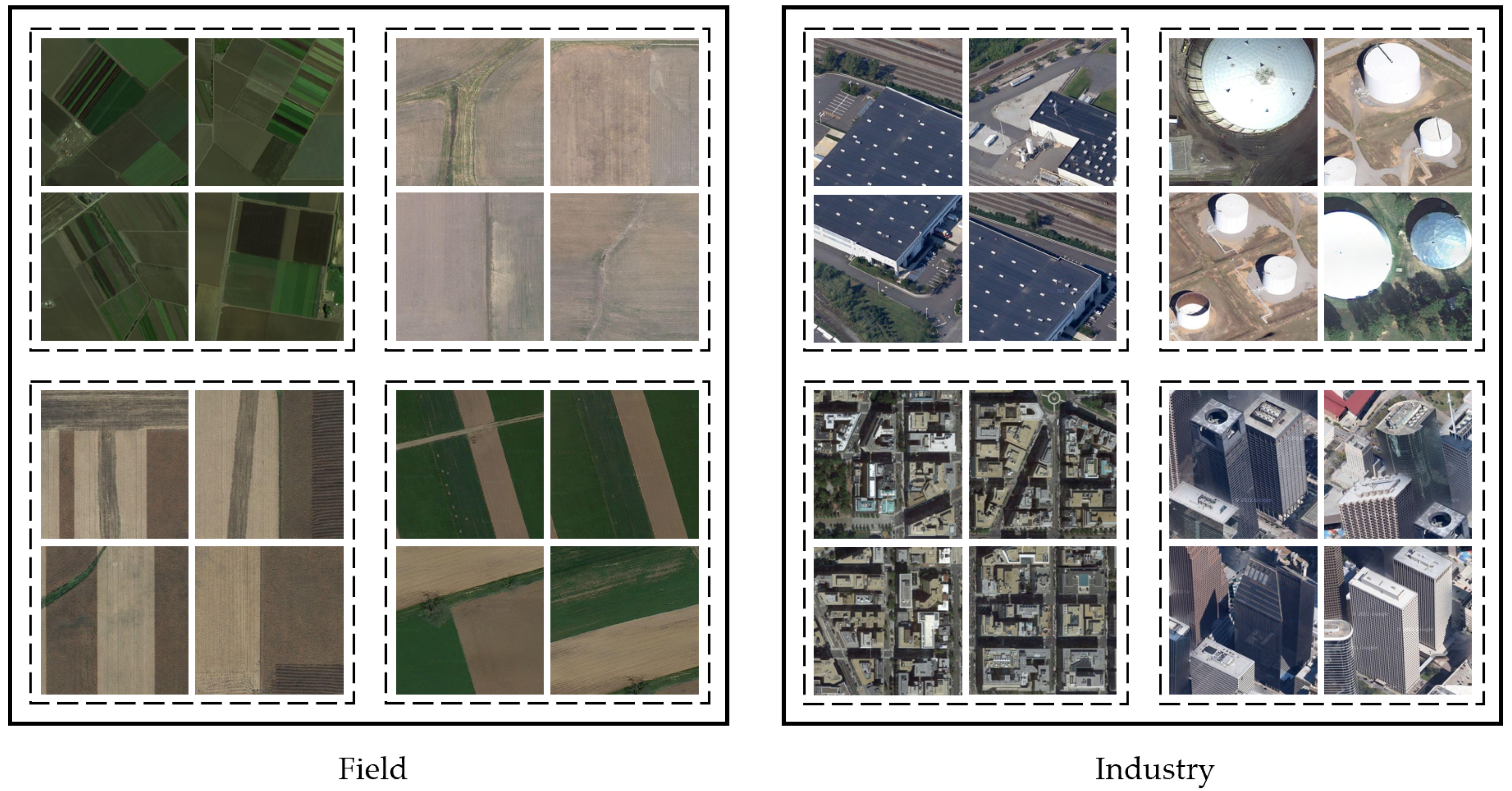
Figure 1.
Intra-class differences and aggregation on RSSCN7. The solid boxes show the images of the field and the industry class, respectively. It can be found that in the same class, the features of samples in the same dotted box are similar, while the features of samples in different dotted boxes are relatively different.

Figure 2.
The t-SNE visualization on RSSCN7. The points in the figure represent samples and different colors represent different classes. It can be found that the samples of the same classes are scattered, and show a local aggregation.
Figure 2.
The t-SNE visualization on RSSCN7. The points in the figure represent samples and different colors represent different classes. It can be found that the samples of the same classes are scattered, and show a local aggregation.

Figure 3.
The AMP method framework. The top half of the figure is the initialization module, and the backbone network maps the sample features into the embedding space, as shown in (a). The yellow and green in the figure represent two classes of samples, the gray-shaded parts are the clusters after performing the clustering algorithm, as show in (b). The lower half of the figure represents the training phase. (c) shows the initial training data in a batch. We synthesize the samples intra-cluster within the batch based on the information obtained in the initialization phase, and the dashed border indicates the synthesized samples, as shown in (d). After the synthesis phase, we assign a proxy to each cluster to express the intra-cluster features. The triangle in (e) represents the proxy, the square in (f) represents the overall features of the class, and the thickness of the line between the square and the triangle represents the weight of the proxy.

Figure 4.
Intra-cluster synthesis. We select similar samples in batches, divide them by the clusters obtained from the initialization module, and use the strategy of intra-cluster synthesis, which is performed with a controllable degree of randomness. The distribution of samples before synthesis is shown in the left figure, where each color represents a class of sample features and different shapes indicate different clusters. The middle image represents our proposed synthesis method with random factor, where is the sample synthesized through samples and , and the right image shows the distribution of the samples synthesized by the green class, and we use the dashed edges to indicate the synthesized samples.

Figure 5.
and are the two original samples, the circle with a dashed border represents the synthesized sample, and the dashed straight line represents the range of the sample synthesis. Assuming that , the range of sample synthesis is between and , and the synthesis location is completely determined by the random parameter r. Assuming that , the range of synthesis locations is reduced by half. Assuming that , the sample is synthesized at the midpoint of and .

Figure 6.
Example images of the UCM dataset: (1) agricultural, (2) airplane, (3) baseball diamond, (4) beach, (5) buildings, (6) chaparral, (7) dense residential, (8) forest, (9) freeway, (10) golf course, (11) harbor, (12) intersection, (13) medium residential, (14) mobile home park, (15) overpass, (16) parking lot, (17) river, (18) runway, (19) sparse residential, (20) storage tanks, (21) tennis court.

Figure 7.
Example images of the RSSCN7 dataset: (1) Grass, (2) Field, (3) Industry, (4) River Lake, (5) Forest, (6) Resident, (7) Parking.
Figure 7.
Example images of the RSSCN7 dataset: (1) Grass, (2) Field, (3) Industry, (4) River Lake, (5) Forest, (6) Resident, (7) Parking.

Figure 8.
Example images of the AID dataset: (1) Airport, (2) Bare Land, (3) Baseball Field, (4) Beach, (5) Bridge, (6) Center, (7) Church, (8) Commercial, (9) Dense Residential, (10) Desert, (11) Farmland, (12) Forest, (13) Industrial, (14) Meadow, (15) Medium Residential, (16) Mountain, (17) Park, (18) Parking, (19) Playground, (20) Pond, (21) Port, (22) Railway Station, (23) Resort, (24) River, (25) School, (26) Sparse Residential, (27) Square, (28) Stadium, (29) Storage Tanks, (30) Viaduct.

Figure 9.
Example images of the PatternNet dataset: (1) airplane, (2) baseball field, (3) basketball court, (4) beach, (5) bridge, (6) cemetery, (7) chaparral, (8) Christmas tree farm, (9) closed road, (10) coastal mansion, (11) crosswalk, (12) dense residential, (13) ferry terminal, (14) football field, (15) forest, (16) freeway, (17) golf course, (18) harbor, (19) intersection, (20) mobile home park, (21) nursing home, (22) oil gas field, (23) oil well, (24) overpass, (25) parking lot, (26) parking space, (27) railway, (28) river, (29) runway, (30) runway marking, (31) shipping yard, (32) solar panel, (33) sparse residential, (34) storage tank, (35) swimming pool, (36) tennis court, (37) transformer station, (38) wastewater treatment plant.

Figure 10.
The number of proxies assigned to each class in the UCMD dataset by our proposed adaptive multi-proxy assignment method.
Figure 10.
The number of proxies assigned to each class in the UCMD dataset by our proposed adaptive multi-proxy assignment method.

Figure 11.
The number of proxies assigned to each class in the AID dataset by our proposed adaptive multi-proxy assignment method.
Figure 11.
The number of proxies assigned to each class in the AID dataset by our proposed adaptive multi-proxy assignment method.

Figure 12.
The number of proxies assigned to each class in the PatternNet dataset by our proposed adaptive multi-proxy assignment method.
Figure 12.
The number of proxies assigned to each class in the PatternNet dataset by our proposed adaptive multi-proxy assignment method.

Figure 13.
The number of proxies assigned to each class in the RSSCN7 dataset by our proposed adaptive multi-proxy assignment method.
Figure 13.
The number of proxies assigned to each class in the RSSCN7 dataset by our proposed adaptive multi-proxy assignment method.

Figure 14.
Examples of UCMD retrieval results. Column 1 is the query sample, columns 2–4 are the success cases of our method, and columns 5–7 are the failure cases.
Figure 14.
Examples of UCMD retrieval results. Column 1 is the query sample, columns 2–4 are the success cases of our method, and columns 5–7 are the failure cases.

Figure 15.
Examples of RSSCN7 retrieval results. Column 1 is the query sample, columns 2–4 are the success cases of our method, and columns 5–7 are the failure cases.
Figure 15.
Examples of RSSCN7 retrieval results. Column 1 is the query sample, columns 2–4 are the success cases of our method, and columns 5–7 are the failure cases.

Figure 16.
Examples of AID retrieval results. Column 1 is the query sample, columns 2–4 are the success cases of our method, and columns 5–7 are the failure cases.
Figure 16.
Examples of AID retrieval results. Column 1 is the query sample, columns 2–4 are the success cases of our method, and columns 5–7 are the failure cases.

Figure 17.
Examples of PatternNet retrieval results. Column 1 is the query sample, columns 2–4 are the success cases of our method, and columns 5–7 are the failure cases.
Figure 17.
Examples of PatternNet retrieval results. Column 1 is the query sample, columns 2–4 are the success cases of our method, and columns 5–7 are the failure cases.

Figure 18.
A t-SNE visualization of the proposed method. (a–e) are the t-SNE visualizations of the first five epochs of all classes in the dataset UCMD. (f–i) are the t-SNE visualizations at the 10th, 20th, 30th, and 40th epochs, respectively. Different colors in the diagram represent different classes.


Table 1.
Experiment settings.
| Settings Name | Value |
|---|---|
| Batch size | 150 |
| Embedding size | 512 |
| Epoch | 50 |
| Evaluation metric | Recall@K mAP mAP@R |
| Dataset division method | 50% for training and 50% for testing in each class |
| 80% for training and 20% for testing in each class | |
| 50% classes for training and the other 50% of classes for testing |
Table 2.
Validation of the cluster algorithm on UCMD and AID. The best results are shown in bold.
| UCMD | AID | |||||||||
|---|---|---|---|---|---|---|---|---|---|---|
| R@1 | R@2 | R@4 | R@8 | mAP | R@1 | R@2 | R@4 | R@8 | mAP | |
| K-means | 97.82 | 98.67 | 99.25 | 99.71 | 94.56 | 95.95 | 96.80 | 97.65 | 98.73 | 94.15 |
| DBSCAN | 97.78 | 98.63 | 99.19 | 99.65 | 94.51 | 95.96 | 96.81 | 97.62 | 98.69 | 93.99 |
| BIRCH | 97.81 | 98.61 | 99.17 | 99.68 | 94.47 | 95.87 | 96.77 | 97.61 | 98.67 | 94.08 |
Table 3.
Validation of the sample synthetic method on UCMD and AID. The best results are shown in bold.
Table 3.
Validation of the sample synthetic method on UCMD and AID. The best results are shown in bold.
| Method | UCMD | AID | ||||||||
|---|---|---|---|---|---|---|---|---|---|---|
| R@1 | R@2 | R@4 | R@8 | mAP | R@1 | R@2 | R@4 | R@8 | mAP | |
| No synthetic | 97.38 | 98.31 | 98.86 | 99.59 | 93.13 | 95.27 | 96.37 | 97.21 | 97.67 | 93.13 |
| synthetic | 97.59 | 98.39 | 98.99 | 99.63 | 93.74 | 95.61 | 96.49 | 97.48 | 98.17 | 93.62 |
| synthetic+a | 97.82 | 98.67 | 99.25 | 99.71 | 94.56 | 95.95 | 96.80 | 97.65 | 98.73 | 94.15 |
Table 4.
Validation of the parameter a on UCMD and AID. The best results are shown in bold.
| a | UCMD | AID | ||||||||
|---|---|---|---|---|---|---|---|---|---|---|
| R@1 | R@2 | R@4 | R@8 | mAP | R@1 | R@2 | R@4 | R@8 | mAP | |
| 0.2 | 97.62 | 98.43 | 99.09 | 99.65 | 93.85 | 95.66 | 96.52 | 97.51 | 98.22 | 93.77 |
| 0.4 | 97.71 | 98.53 | 99.17 | 99.68 | 94.12 | 95.79 | 96.71 | 97.58 | 98.55 | 93.92 |
| 0.6 | 97.82 | 98.67 | 99.25 | 99.71 | 94.56 | 95.95 | 96.80 | 97.65 | 98.73 | 94.15 |
| 0.8 | 97.81 | 98.63 | 99.21 | 99.68 | 94.51 | 95.92 | 96.81 | 97.63 | 98.70 | 94.10 |
| 1 | 97.73 | 98.57 | 99.13 | 99.61 | 94.29 | 95.73 | 96.67 | 97.53 | 98.46 | 93.88 |
Table 5.
Validation of the number of proxy and adaptive proxy methods on UCMD and AID. The best results are shown in bold.
Table 5.
Validation of the number of proxy and adaptive proxy methods on UCMD and AID. The best results are shown in bold.
| UCMD | AID | |||||||||
|---|---|---|---|---|---|---|---|---|---|---|
| R@1 | R@2 | R@4 | R@8 | mAP | R@1 | R@2 | R@4 | R@8 | mAP | |
| 1 | 97.42 | 98.34 | 98.98 | 99.57 | 93.07 | 95.27 | 96.37 | 97.21 | 97.67 | 93.13 |
| 2 | 97.55 | 98.41 | 99.05 | 99.59 | 93.32 | 95.42 | 96.46 | 97.33 | 97.93 | 93.54 |
| 3 | 97.72 | 98.52 | 99.12 | 99.62 | 93.68 | 95.73 | 96.61 | 97.45 | 98.41 | 93.82 |
| 4 | 97.67 | 98.49 | 99.11 | 99.63 | 93.71 | 95.75 | 96.59 | 97.47 | 98.37 | 94.05 |
| 5 | 97.69 | 98.51 | 99.13 | 99.61 | 93.75 | 95.78 | 96.62 | 97.46 | 98.39 | 94.01 |
| adaptive | 97.82 | 98.67 | 99.25 | 99.71 | 94.56 | 95.95 | 96.80 | 97.65 | 98.73 | 94.15 |
Table 6.
Validation of the proxy weighting method on UCMD and AID. The best results are shown in bold.
Table 6.
Validation of the proxy weighting method on UCMD and AID. The best results are shown in bold.
| Method | UCMD | AID | ||||||||
|---|---|---|---|---|---|---|---|---|---|---|
| R@1 | R@2 | R@4 | R@8 | mAP | R@1 | R@2 | R@4 | R@8 | mAP | |
| average | 97.51 | 98.32 | 98.99 | 99.53 | 93.41 | 95.37 | 96.46 | 97.37 | 98.03 | 93.56 |
| adaptive | 97.82 | 98.67 | 99.25 | 99.71 | 94.56 | 95.95 | 96.80 | 97.65 | 98.73 | 94.15 |
Table 7.
Recall@K(%), mAP, and mAP@R performance comparison on UCMD and AID. The best results are shown in bold.
Table 7.
Recall@K(%), mAP, and mAP@R performance comparison on UCMD and AID. The best results are shown in bold.
| Method | UCMD (50-50) | AID (80-20) | ||||||||||
|---|---|---|---|---|---|---|---|---|---|---|---|---|
| R@1 | R@2 | R@4 | R@8 | mAP | mAP@R | R@1 | R@2 | R@4 | R@8 | mAP | mAP@R | |
| Triplet Loss [48] | 92.58 | 94.58 | 95.91 | 98.49 | 82.36 | 78.34 | 87.74 | 91.18 | 95.26 | 96.04 | 76.95 | 69.39 |
| N-pair Loss [53] | 95.38 | 96.76 | 97.55 | 98.86 | 85.35 | 81.93 | 90.93 | 92.98 | 95.15 | 96.83 | 82.31 | 78.13 |
| LS Loss [49] | 96.12 | 97.29 | 98.15 | 99.01 | 87.84 | 84.49 | 92.77 | 94.05 | 95.64 | 96.97 | 83.92 | 81.09 |
| BIER [62] | 80.31 | 85.28 | 90.11 | 91.65 | 75.72 | 58.98 | 80.72 | 86.39 | 92.01 | 95.38 | 68.88 | 59.24 |
| A-BIER [63] | 86.52 | 89.96 | 92.61 | 94.76 | 80.82 | 72.11 | 82.28 | 89.51 | 93.55 | 96.37 | 71.59 | 70.51 |
| DCES [64] | 87.45 | 91.02 | 94.27 | 96.32 | 81.53 | 78.93 | 85.39 | 91.02 | 95.27 | 96.63 | 74.28 | 72.53 |
| ABE [65] | 93.71 | 95.57 | 96.96 | 98.32 | 86.53 | 82.91 | 88.33 | 91.39 | 95.56 | 96.89 | 77.83 | 76.91 |
| MS Loss [29] | 96.84 | 97.98 | 98.36 | 99.02 | 90.04 | 85.12 | 93.23 | 94.57 | 95.81 | 97.18 | 87.18 | 84.32 |
| Proxy-NCA Loss [33] | 96.09 | 97.27 | 98.09 | 99.13 | 88.36 | 83.49 | 91.85 | 93.11 | 95.43 | 96.96 | 83.47 | 82.61 |
| SoftTriple Loss [39] | 96.21 | 96.98 | 97.84 | 98.98 | 89.09 | 82.61 | 92.12 | 93.84 | 95.46 | 96.82 | 84.09 | 83.82 |
| Proxy Anchor Loss [32] | 97.22 | 98.19 | 98.75 | 99.42 | 92.41 | 87.35 | 95.12 | 96.29 | 97.11 | 97.47 | 92.85 | 87.12 |
| Our Method | 97.82 | 98.67 | 99.25 | 99.71 | 94.56 | 90.43 | 95.95 | 96.80 | 97.65 | 98.73 | 94.15 | 90.18 |
Table 8.
Recall@K(%), mAP, and mAP@R performance comparison on RSSCN7 and PatternNet with different Dataset division method.
Table 8.
Recall@K(%), mAP, and mAP@R performance comparison on RSSCN7 and PatternNet with different Dataset division method.
| Dataset | R@1 | R@2 | R@4 | R@8 | mAP | mAP@R |
|---|---|---|---|---|---|---|
| RSSCN7 (50-50) | 94.64 | 96.25 | 97.85 | 98.57 | 90.71 | 82.76 |
| RSSCN7 (80-20) | 95.14 | 97.36 | 98.43 | 99.01 | 92.64 | 85.67 |
| PatternNet (50-50) | 99.65 | 99.79 | 99.83 | 99.88 | 99.55 | 99.01 |
| PatternNet (80-20) | 99.87 | 99.88 | 99.90 | 99.91 | 99.74 | 99.51 |
Table 9.
Recall@K(%), mAP, and mAP@R performance for invisible classes on RSSCN7, UCMD, AID, and PatternNet. A total of 50% of classes were for training and the other 50% of classes were for testing.
Table 9.
Recall@K(%), mAP, and mAP@R performance for invisible classes on RSSCN7, UCMD, AID, and PatternNet. A total of 50% of classes were for training and the other 50% of classes were for testing.
| Dataset | R@1 | R@2 | R@4 | R@8 | mAP | mAP@R |
|---|---|---|---|---|---|---|
| RSSCN7 | 96.92 | 98.83 | 99.58 | 99.92 | 74.32 | 55.87 |
| UCMD | 93.40 | 96.10 | 97.70 | 98.70 | 57.21 | 40.56 |
| AID | 87.93 | 93.24 | 96.21 | 98.11 | 48.29 | 34.21 |
| PatternNet | 99.11 | 99.57 | 99.76 | 99.84 | 76.87 | 65.32 |
Publisher’s Note: MDPI stays neutral with regard to jurisdictional claims in published maps and institutional affiliations. |
© 2022 by the authors. Licensee MDPI, Basel, Switzerland. This article is an open access article distributed under the terms and conditions of the Creative Commons Attribution (CC BY) license (https://creativecommons.org/licenses/by/4.0/).
Share and Cite
MDPI and ACS Style
Li, X.; Wei, S.; Wang, J.; Du, Y.; Ge, M. Adaptive Multi-Proxy for Remote Sensing Image Retrieval. Remote Sens. 2022, 14, 5615. https://doi.org/10.3390/rs14215615
AMA Style
Li X, Wei S, Wang J, Du Y, Ge M. Adaptive Multi-Proxy for Remote Sensing Image Retrieval. Remote Sensing. 2022; 14(21):5615. https://doi.org/10.3390/rs14215615
Chicago/Turabian StyleLi, Xinyue, Song Wei, Jian Wang, Yanling Du, and Mengying Ge. 2022. "Adaptive Multi-Proxy for Remote Sensing Image Retrieval" Remote Sensing 14, no. 21: 5615. https://doi.org/10.3390/rs14215615
Note that from the first issue of 2016, this journal uses article numbers instead of page numbers. See further details here.