Coupling and Coordination Relationships between Urban Expansion and Ecosystem Service Value in Kashgar City

Abstract

The growing urbanization of oasis cities in arid and semi-arid regions of Northwest China has an adverse influence on the fragile local ecological system. Therefore, improved understanding of the coupling and coordination between urban expansion (UE) and ecosystem services value (ESv) is critical to long term sustainable development. Here, we study the urbanization trend of a typical oasis city of Northwest China (Kashgar) using Landsat TM/ETM+/OLI imagery from 1990 to 2015. Land use types are classified and the spatio-temporal features of UE are analyzed; ESv of each land use types and the ecosystem services function (ESf) are determined; the driving factors of UE and the spatio-temporal change of ESv are analyzed; and the coupling and coordination relationship between UE and ESv is quantitatively determined. Results show that: (1) The land use structure has changed significantly between 1990 and 2015, with construction land (40.51 km²) showing the highest growth and farmland (28.42 km²). (2) UE values during 2000–2005 (16.65 km²) and 2010–2015 (21.09 km²) are relatively large, and during 1990–2015, the city extended from the center to the outskirts at a dynamic growth rate of 13.17% and a comprehensive expansion index of 1.54‰. (3) The total ESv was reduced by CNY 35.76 million (USD ~ 5.26 million), ranked from high to low as: waste treatment (CNY 9.94 million, USD ~1.46 million), water source conservation (CNY 7.95 million, USD ~ 1.17 million), soil formation (CNY 4.60 million, USD ~ 0.68 million), biodiversity protection (CNY 3.37 million, USD ~ 0.5 million), climate regulation (CNY 3.15 million, USD ~ 0.46 million), food production (CNY 2.83 million, USD ~ 0.42 million), gas regulation (CNY 1.96 million, USD ~ 0.29 million), entertainment and leisure (CNY 1.26 million, USD ~ 0.19 million), and raw materials (CNY 0.68 million, USD ~ 0.1 million). (4) The coupling degree between UE and ESv is relatively small (<0.5), though this value has increased yearly. The coordination degree between UE and ESv is relatively low, indicating that UE already poses a serious danger to the ecological environment. (5) The rapid growth of the population and economy and government policies are the main driving factors of intensive UE. Increasing climatic factors such as precipitation, temperature, and runoff impact ESv in some positive ways whereas UE leads to a reduction of ESv. Our results here can help to guide long-term sustainable development of arid regions, reasonable urban planning of oasis cities, and protection of the local ecological environment.

1. Introduction

Urban expansion (UE) is an important indicator of the urbanization process, and urban land use change is the most direct manifestation of UE [1]. Bourne [2] demonstrated that forms of UE includes axial expansion, concentric circular expansion, fan-shaped expansion, and multi-core expansion. Previous studies have suggested that: (1) the urban spatial shape includes four modes: belt expansion, circle expansion, cluster expansion, and sprawling expansion; (2) the main driving forces of UE are urban geographic environment, farmland quality, economic conditions, and population growth rate; (3) stable economic development, superior urban location, and environmental conditions have a significant role in promoting UE [3,4,5,6,7].

Recently, China has experienced significant UE, with three key aspects: urban spatial form, structure, and spatial variation characteristics. Gu et al. [8] proposed that axial expansion and outward expansion are the two main forms of UE in China. Liu et al. [9] determined that UE has four types: infill, extension, corridor, and satellite town. Abudureyimu et al. [10] analyzed the features and driving force of UE in Yining City using remote sensing (RS) imagery from 1990 to 2015, showing that occupied farmland, woodland, and unused land, along with economic development and population growth, are the main driving factors of UE. Gao et al. [11] used DMSP/OLS night light RS data to extract urban pixels of 25 countries and regions in Central Asia, West Asia, and Western China, and explored the expansion type, expansion intensity, expansion form, and driving mechanism of certain cities in these arid regions.

UE causes changes in urban built-up areas and urban spatial patterns, which in turn can impact the status, characteristics, and functions of the urban ecosystem. The ecological effects of UE include the atmosphere, soil, water, biodiversity, and ecosystem services. Ecosystem services value (ESv) refers to the advantages that humans derive directly or indirectly from the ecology, such as the input of valuable substances and energy into the economic and social system, the acceptance and transformation of waste from the economic and social system, and direct services to human society [12]. UE affects basic functions, such as energy flow and material circulation of the ecosystem, and also has impacts on the ecosystem services function (ESf), such as waste treatment, water conservation, climate regulation, soil formation, food production, and recreation [13]. Therefore, changes in urban ESv by the process of rapid urbanization can replicate the changes in ecological effects caused by UE.

The UE process is a significant global-scale threat to ecological environments, particularly in urbanizing arid regions with fragile ecological environments [14,15]. The impact of UE on the urban ecological environment is mainly measured by ESv [16]. UE tends to scale back ESv, thereby negatively impacting the urban ecological environment [17,18,19,20]. Reasonable development of urban land and establishment of urban green spaces is thus crucial in protecting urban ecosystems.

The coupling and coordinating link between UE and natural environment systems in rapidly urbanized areas has been the subject of extensive research since the 1990s. Many studies [21,22,23] have systematically analyzed nonlinear coupling relationships and characteristics between ecological environmental systems (natural systems) of urban agglomerations and urbanization systems (humanistic systems). The stress and promotion effect of UE on the ecological environment; the restraint and carrying effect of ecological environments on UE; the coupling evaluation, mechanism, law, and simulation between UE and ecological environments; and the impact of urban construction land growth, land transfer distribution, and land use structure change on ecological landscapes [24,25,26,27] are examples of couplings between UE and ecological environments in rapidly urbanized areas.

The arid and semi-arid lands of Northwest China suffer from a significant lack of water resources, and have very dry climates, low precipitation, scarce biological species, small vegetation coverage, and limited available land resources. These cities may be thought of as “oasis cities” which are distributed according to the limited water resources and specific geographic location. As a result of increased investment by national and local governments, the rate of urbanization and population agglomeration has accelerated, and the impacts of UE have increased [28,29,30]. Increasing UE has detrimental consequences for the local ecological environment [31]. However, a consideration of the effects of UE on the ecological environment for oasis cities in the arid and semi-arid regions of Northwest China has received limited attention [32,33,34]. Kashgar, in western China, has experienced rapid urbanization and significant urban spatial expansion. Ecological land has been increasingly replaced by urban expanded land, which has impacted the ecological environment. Therefore, the coordinated development of local urbanization and ecological environment is a key issue for the sustainable development of Kashgar city. It is thus vital to evaluate the degree and range of the impact of UE on the ecological environment using quantitative analysis methods.

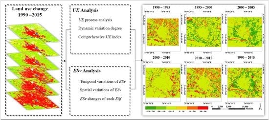
Here, we used long-record RS image data and determined the ESf coefficient of the terrestrial ecosystem of the Kashgar region. The coupling degree and coordination degree are determined by using a capacity coupling model. The main goals of this study are: (1) determine the UE of the long-term spatio-temporal dynamic processes of Kashgar and reveal fundamental causative mechanisms, (2) analyze the changes of ESv of each land use type and each ESf caused by long-term UE processes, (3) calculate the impact of UE on ESv, and (4) examine the coupling and coordination links between UE and ESv. Our results will guide the best use of limited land resources, help to protect vulnerable ecological ecosystems, promote sustainable development, and provide scientific recommendations for successful ecological preservation.

2. Study Area and Data

2.1. Study Area

Kashgar, located near the Taklimakan Desert, is the westernmost border city in China. Its geographical location is between 73°20′~79°57′ E and 35°20′~40°18′ N (Figure 1). The total area of the city is 651 km² and its average altitude is 1289.5 m. The region is a warm temperate continental arid climate, with high temperatures and infrequent precipitation. The annual average temperature is 11.7 °C, the annual average precipitation is 61.5 mm, and the annual evaporation is 2500 mm.

We focused here on the urban built-up area, as the human activity is intensive in the city center, whereas the majority of the urban outskirts are desert or barren terrain.

Table 1. Study area extracted from RS images.

Administrative Area (km2)	Urban Built-Up Area (km2)	Proportion of Urban Built-Up Area (%)	Urban Built-Up Area Extracted from RS Images
			Longitude	Latitude	Area (km2)
199.38	62.73	31.46	39°25′48″N–39°30′17″N	75°55′49″E–76°3′6″E	85.32

shows that the urban built-up area only accounts for 31.46% of the total administrative area, and in non-built-up areas, there is essentially little change in land use types.

2.2. Data

We classified land use using images from Landsat TM/ETM+/OLI (

Table 2. Remote sensing data used.

Path/Row	Satellite and Sensor	Acquisition Time	Band Combination	Spatial Resolution	Cloud Coverage
149/33	Landsat-4 TM	7 August 1990	743	30 m	<10%
	Landsa-t4 TM	9 November 1995
	Landsat-4 TM	14 May 2000
	Landsat-5 ETM+	9 September 2005
	Landsat-5 ETM+	22 August 2010
	Landsat-8 OLI	11 July 2015	654	Multi-spectral: 30 m Panchromatic band: 15 m

) obtained from the United States Geological Survey (https://www.usgs.gov/). The equivalent ESv coefficient and the land use classification data are used to calculate ESv. Socioeconomic data is collected from the Xinjiang Statistical Yearbook (1991–2020) (http://tjj.xinjiang.gov.cn/) and the government work report (https://www.xinjiang.gov.cn/).

3. Methods

3.1. Land Use Classification

We used 1:10,000 topographic maps and the ENVI4.8 professional software to perform geometric and atmospheric corrections on the original RS images. The average position error of the image is controlled to be below one pixel to improve the accuracy of the classification. We consider color, size, shape, structure, shadow, and other spatial distribution characteristics of each land used type, as well as land use planning maps and Google Earth images, and apply a maximum likelihood approach of supervised classification to classify the images. We divide the land use types of Kashgar into five major categories using the system for classifying land resources developed by the Chinese Academy of Sciences “Remote Sensing National Resources and Environment Remote Sensing” [35]: woodland, construction land, water body, farmland, and unused land. For each land used type, more than 200 identified samples were chosen, all of which are representative and geographically homogenous. Results are filtered and combined after classification to increase picture classification accuracy, which are further validated using field sample data.

Table 3. Classification accuracy of remote sensing imagery.

Accuracy Index	1990	1995	2000	2005	2010	2015
Kappa coefficient	0.846	0.865	0.887	0.868	0.890	0.846
Overall accuracy (%)	85.79	87.61	88.36	86.61	89.24	85.08

shows the Kappa coefficient and overall accuracy (between 0 and 1; the closer to 1, the more accurate the classification), which are all relatively high, indicating that the classification accuracy is reliable, and the data can be employed for further analysis.

3.2. UE Indices

3.2.1. The Dynamic Variation Degree

The dynamic variation degree of UE refers to the annual rate of change of land use type [36]:

$$K=\frac{U_b-U_a}{U_a}\times \frac{1}{T}\times 100\%$$

(1)

where K is the dynamic variation degree of UE; U_a and U_b are the area (unit: km²) of the construction land at the study year of a and b, respectively; and T is the length between a and b. According to K, the UE is divided into four expansion types (

Table 4. Classification of UE types.

Dynamic Variation Degree (K) (%)	Expansion Type
K ≤ 8	Slow
8 < K ≤ 14	Medium
14 < K ≤ 20	Fast
K > 20	High speed

).

3.2.2. The Comprehensive Expansion Index

The comprehensive expansion index reflects UE by considering expanded land area, the urban land area in the beginning of the study period, and the total urban land area [37]:

$$CEI=\frac{U_b-U_a}{U_a}\times \frac{1}{U}\times \frac{1}{T}\times 1000‰$$

(2)

where CEI is the comprehensive expansion index of urban land types, U_a and U_b are the area (unit: km²) of the construction land at the study year of a and b, respectively, and T is the length between a and b. According to CEI, we divide UE into four expansion types (

Table 5. Classification of UE types.

Comprehensive Expansion Index (CEI)(%)	Expansion Type
CEI ≤ 0.2	Slow
0.2 < CEI ≤ 0.35	Medium
0.35 < CEI ≤ 0.5	Fast
CEI > 0.5	High speed

).

3.3. Evaluation Method of Urban ESv

To calculate the ESv of each land used type, we first identify the ESf type and the accompanying coefficient standard. Costanza et al. [38,39] proposed a global ESv evaluation method. Xie et al. [40,41] computed ESf and corresponding coefficients of the terrestrial ecosystems of China. Mamat et al. [42], Eziz et al. [33], and Mamat et al. [32] proposed ESf and corresponding coefficients per unit area of different land used types in oasis cities in the arid and semi-arid regions in northwest China (

Table 6. Ecosystem function per unit area (unit: CNY·hm⁻²·a⁻¹).

ESf	Construction Land	Farmland	Woodland	Water Body	Unused Land
Gas regulation	0.0	484.0	1940.1	0.0	27.0
Climate regulation	0.0	861.6	1827.8	445.3	58.4
Water conservation	0.0	580.9	1836.8	19,749.1	31.4
Soil formation	0.0	1413.4	1805.4	9.7	76.4
Waste treatment	0.0	1587.7	772.5	17,619.3	116.8
Biodiversity protection	0.0	687.3	2025.4	2410.6	179.6
Food production	0.0	968.1	148.2	96.8	9.0
Raw materials	0.0	96.8	1338.3	9.7	18.0
Recreation	82.6	9.7	934.1	4201.5	107.8
Total	82.6	6689.5	12,628.6	44,542.0	624.4

) as:

$$ESvk={{\displaystyle \sum }}_{f=1}^n\left(A_k\times V{C}_{kf}\right)$$

(3)

$$ESvf={{\displaystyle \sum }}_{k=1}^m\left(A_k\times V{C}_{kf}\right)$$

(4)

where ESvk is the ESv of land used type k, ESvf is the ESv of service function type f, VC_kf is the ecosystem function (CNY·ha⁻²·a⁻¹) for land used type k, and A_k is the area (hm²) for land used type k.

3.4. Evaluation Model of Coupling Coordination Degree

Coupling can be classified into four types: (1) low-level coupling, (2) antagonism, (3) running-in, and (4) high-level coupling, based on the degree of coupled interaction. Here, we employ both a coupling model and coordination degree model.

3.4.1. Coupling Degree Model

The degree of coupling reflects the mutual influence of two systems. According to the concept of capacity coupling in physics, we applied a coupling degree model between UE and ESv [43]:

$$C=\sqrt{\left(\left(U\times E\right)/{(U+E)}^2\right)}$$

(5)

Here, U and E denote the quantity of UE and the associated ESv change during the same period and C refers to the coupling degree between UE and ESv, and C∈[0,1].

The greater the value of C, the more coordinated the development of UE and ESv; when C = 1, the coupling degree is the largest, and UE and ESv tend to develop in an orderly manner; when C = 0, the coupling degree is the smallest, and the two systems are unrelated and the system development is disordered. The coupling degree can be classified into four types according to its value [44] (

Table 7. Classification system of coupling degree.

Coupling Degree (C)
Range of Values	Coupling Degree
C = 0	No mutual influence
0 < C ≤ 0.3	Low-level coupling
0.3 < C ≤ 0.5	Antagonistic Coupling
0.5 < C ≤ 0.8	Running in
0.8 < C < 1	High-level coupling
C = 1	Strong correlation

).

3.4.2. Coordination Model

Coupling cannot directly measure the level of mutual coordination between the two systems, as they may be staggered, dynamically changing, and unbalanced. The coupling degree of the two subsystems will be high if only the coupling degree is evaluated, resulting in “false coordination” between UE and ESv. The coupling coordination degree model is based on the coupling degree [44]:

$$T=\sqrt{\alpha X+\beta Y}$$

(6)

$$D=\sqrt{C\times T}$$

(7)

where D is the degree of coordination, T is the comprehensive coordination index of the two systems, and α and β are undetermined coefficients with α + β = 1. We use a value of 0.5 for both α and β, in line with previous studies. The uniform distribution function method is used to classify nine levels of coordination (

Table 8. Coordination degree classification.

Coordination Degree (D)
Section	Range of Values	Coordination Degree
Maladjusted recession area	0.0 ≤ D ≤ 0.09	Extreme disorder
	0.1 ≤ D ≤ 0.19	Severe disorder
	0.2 ≤ D ≤ 0.29	Moderate disorder
	0.3 ≤ D ≤ 0.39	Mild disorder
Transition area	0.4 ≤ D ≤ 0.49	Verge of disorder
	0.5 ≤ D ≤ 0.59	Reluctantly coordinated
Coordinated development area	0.6 ≤ D ≤ 0.69	Primary coordinated
	0.7 ≤ D ≤ 0.79	Intermediate coordinated
	0.8 ≤ D ≤ 0.89	Good coordinated

).

The flowchart of this research is shown in Figure 2.

4. Results

4.1. Urban Land Use Classification Change

The ArcGIS 10.3 software is used to map the land use classification results (Figure 3), and land use parameters are generated (Figure 4).

The land use structure of Kashgar has shifted dramatically between 1990 and 2015. There are a few notable points:

(1) The area of construction land grew, particularly between 2000 and 2015, when the increase (approximately 39.01 km²) was the largest and the annual average growth rate (approximately 18.99%) was the most rapid.

(2) There was a major change in the area of agriculture. It shrank from 48.82 km² in 2000 to 20.40 km² in 2015, with a total reduction of 28.42 km², more than half of the original farmland area.

(3) The change of woodland area is uncertain, as it increased in the early and later periods and decreased in the middle period. The most notable changes occurred during 1990–1995 when the area increased from 13.22 km² to 23.35 km², a total increase of 10.13 km², with an annual average increase rate of 15.33%. After this time, the area decreased.

(4) Water body areas steadily decreased from 4.12 km² (in 1990) to 1.21 km² (in 2015), a total reduction of 2.91 km².

(5) Unused land decreased from 7.63 km² in 2015 to 0.72 km² in 2015, a total reduction of 6.91 km². This suggests that the majority of previously undeveloped area has now been utilized. However, it increased slightly in 2000, as a small area of unused land appeared in the northeastern part of the city, which was later occupied by construction land.

Thus, the acreage and share of construction land increased, whereas farmland decreased; the latter made significant contributions to UE.

4.2. Spatio-Temporal Characteristics of UE

4.2.1. UE Process Analysis

Spatial overlay analysis was performed between the construction map layers during different periods by using ArcGIS 10.3 software, with results shown in Figure 5 and Figure 6.

The UE pattern is concentric, as construction land expanded from the center to the outskirts, and newly added construction land is evenly distributed around the original built-up area of the city. This is most likely due to Kashgar’s relatively flat geography and the lack of mountains to obstruct UE.

The expansion area and rate can be used to calculate the UE degree. The size and degree of UE vary during each period analyzed due to the disparities in social and economic growth.

(1) The expansion area during 2010–2015 (21.09 km²) and during 2000–2005 (16.65 km²) were larger, whereas the expansion area in the other periods was smaller (1.27 km² in 2005–2010, 1.25 km² in 1995–2000 and 0.25 km² in 1990–1995). During 1990–2015, the construction land area increased by 40.51 km². By 2015, the construction land area was 52.7 km², more than four times the area in 1990 (12.19 km²).

(2) The expansion rates in 2010–2015 and 2000–2005 were also relatively high, at around 24.72% and 19.63%, respectively. In other eras, the expansion ratios were lower (1.48% in 2005–2010, 1.35% in 1995–2000, and 0.4% in 1990–1995).The expansion ratio increased by 47.58% during 1990–2015. By 2015, the proportion of construction land area to the total land area was 61.76%, more than four times the rate in 1990 (14.18%).

4.2.2. Dynamic Variation Degree Analysis

The dynamic variation degree is the annual average change rate of the construction land area in a given period of time compared to the construction land area in the starting stage.

Table 9. Dynamic variation degree and comprehensive expansion index of UE.

Sub-Study Period	Dynamic Variation Degree (D)		Comprehensive Expansion Index (CEI)
	Value (%)	Expansion Type	Value (‰)	Expansion Type
1990–1995	0.67	Slow	0.08	Slow
1995–2000	1.56	Slow	0.18	Slow
2000–2005	24.45	High speed	2.86	High speed
2005–2010	0.76	Slow	0.09	Slow
2010–2015	12.88	Medium	1.51	High speed
1990–2015	13.17	Medium	1.54	High speed

shows that the K values for each study period in increasing order were: K_2000–2005, K_2010–2015, K_1995–2000, K_2005–2010, and K_1990–1995. This indicates that UE in 2000–2005 was a high-speed expansion type, a medium-speed expansion type in 2010–2015, and a slow expansion type during the rest of the study period. Over the entire study period of 25 years, K_1990–2015 = 13.17%, categorized as medium-speed expansion type, indicating that the city consistently increased over the full era.

4.2.3. Comprehensive Expansion Index Analysis

The comprehensive expansion index is defined as the yearly average growth rate of the construction land area changes in a given period of time compared to the starting construction land area and total urban land area. The CEI of each period in increasing order is: CEI_2000–2005, CEI_2010–2015, CEI_1995–2000, CEI_2005–2010, and CEI_1990–1995. This demonstrates that UE in Kashgar increased at a high rate between 2000 and 2005 and at a low rate between 2010 and 2015. Over the entire study period, CEI_1990–2015 was 1.54‰, a high-speed expansion, indicating that the urban land in Kashgar has expanded rapidly in the last 25 years.

4.3. ESv Analysis

Land structure change caused by UE will inevitably have an impact on regional ESv. The total ESv value was calculated using Formulas (3) and (4). Using the ESf coefficients of terrestrial ecosystems in arid and semi-arid regions (Table 6) and the area of different land types (Figure 4), the total ESv value was estimated. The spatial changes of ESv in each period and corresponding ESv changes of each land used type and ESf index are determined by the spatial analysis function in ArcGIS10.3.

4.3.1. Temporal Variations of ESv

The temporal changes of ESv (Figure 7) show that: (1) ESv was significantly high in the early stage and relatively small in the later stage, progressively falling from CNY 68.27 million (USD ~10.04 million) in 1990 to CNY 32.51 million (USD ~4.78 million) in 2015, a total decrease of CNY 35.76 million (USD ~5.26 million), with a 2.09% yearly average decline, suggesting that UE had a harmful impact on the ecological environment. (2) The descending order of ESv by 5-year period is: ESv₁₉₉₅ (CNY 73.59 million, USD ~10.83 million), ESv₁₉₉₀ (CNY 68.26 million, USD ~10.04 million), ESv₂₀₀₀ (CNY 57.96 million, USD ~8.53 million), ESv₂₀₁₀ (CNY 52.73 million, USD ~7.76 million), ESv₂₀₀₅ (CNY 48.12 million, USD ~7.08 million), and ESv₂₀₁₅ (CNY 32.51 million, USD ~4.78 million). (3) Farmland, woodland, and water bodies are the three primary land used types which affect ESv; these three types accounted for 99.15% of the total ESv in 1990 (CNY 67.69 million, USD ~9.96 million), and for 98.52% in 2015 (CNY 32.03 million, USD ~4.71 million). In contrast, construction land and unused land have little impact on total ESv changes and only are a small percentage of the total ESv.

We calculated ESv changes for each five-year period, as well as the total ESv changes from 1990 to 2015 (Figure 8). These findings reveal that: (1) The ESv of Kashgar is dynamic, as the changes of ESv during 1990–1995 and 2005–2010 were positive and ESv increased, whereas the ESv changes of the remaining periods were negative and ESv decreased. (2) The rankings of ESv are: ESv_2000–2015 (CNY −20.22 million, USD ~−2.97 million), ESv_1995–2000 (CNY −15.63 million, USD ~−2.30 million), ESv_2000–2005 (CNY −9.84 million, USD ~ −1.45 million), ESv_1990–1995 (CNY 5.32 million, USD ~0.78 million), and ESv_2005–2010 (CNY 4.61 million, USD ~ 0.68 million). (3) The size of the land use area and the ESf coefficient determine ESv. From 1990 to 2015, ESv _{construction land} (smaller ESf coefficient) increased by CNY ~0.33 million (USD ~0.05 million), ESv _farmland (larger ESf coefficient) decreased by CNY ~19.01 million (USD ~2.8 million), ESv _woodland (larger ESf coefficient) decreased by CNY ~3.69 million (USD ~0.54 million), ESv _{water body} (larger ESf coefficient) decreased by CNY ~12.96 million (USD ~1.91 million), and ESv _{unused land} (larger ESf coefficient) decreased by CNY ~0.43 million (USD ~0.06 million).

4.3.2. Spatial Variations of ESv

We used the ArcGIS 10.3 software to draw the spatial distribution of ESv changes over each of the study periods (Figure 9).

UE was primarily responsible for the change in ESv, and ESv fluctuations correspond to UE trends. ESv typically declines in regions where UE occurs, whereas ESv increases in areas where ecological land increases. Ecosystem function and land use area were used to determine ESv change. The spatial change of ESv is most influenced by areal changes in land used types with high ESf coefficients. The ESf of woodland, farmland, and water bodies are relatively higher, and their ESv made up a higher percentage, indicating that these three different types of land provide additional service value. (Table 6). Comparing Figure 5 and Figure 9, we can see that the expanded area of ESv corresponds to an increase of woodland and water bodies. Thus, the ESv distribution and change in space and time may be determined by UE size and intensity. Typically, the UE process is commonly observed in land used types with high ecosystem function in oasis towns of arid climates, and it has a detrimental effect on ecological systems.

In 1990, regions with significant ESv decline largely corresponded to ecological land (including farmland, woodland, and water bodies) (Figure 9). The extent of development land expanded significantly throughout the rapid urbanization process, whereas the area of ecological land declined significantly. The loss of ESv was directly caused by changes in land structure during the rapid urbanization process of the last 25 years, particularly the reduction of ecological land area induced by UE. This suggests that UE has a negative effect on the ecological environment, especially in recent years.

4.3.3. ESv Change of ESv Indicators

We now consider the ESv values and their corresponding proportion of each ESf index in each period (Figure 10 and Figure 11). For all time periods, ESv and the proportion of four ESf indexes (water conservation, waste treatment, soil formation, and biodiversity protection) are relatively large, whereas the remaining five ESf indexes are relatively small, implying that these four indices are the best representations of ESv changes in Kashgar.

All of the ESv of each ESf index decreased during the past 25 years. The ESv reduction ESf index is ordered as: waste treatment (CNY 9.94 million, USD ~1.46 million), water conservation (CNY 7.95 million, USD~1.17 million), soil formation (CNY 4.60 million, USD ~0.68 million), biodiversity protection (CNY 3.37 million, USD ~0.5 million), climate regulation (CNY 3.15 million, USD ~0.46 million), food production (CNY 2.83 million, USD ~0.42 million), gas regulation (CNY 1.96 million, USD ~ 0.29 million), entertainment (CNY 1.26 million, USD ~ 0.19 million), and raw materials (CNY 0.68 million, USD ~ 0.1 million). The contribution of each ESf index to the total ESv reduction is ordered as: waste treatment (27.81%), water conservation (22.25%), soil formation (12.86%), biodiversity protection (9.43%), climate regulation (8.82%), food production (7.91%), gas regulation (5.49%), entertainment (3.53%), and raw materials (1.91%).

These findings strongly suggests that waste treatment and water conservation, with a combined contribution of 50.06 percent, are the two ESf indexes that contribute the largest proportion of the total ESv change, whereas entertainment and raw materials have the smallest (5.44%). The ESf in Kashgar is thus best described as a regulation service function, since the value of the ecosystem regulation service function is smaller than that of the supply service function.

4.4. Analysis of the Degree of Coupling and Coordination between UE and ESv

We now calculate the coupling degree (C) and coordination degree (D) in each time period between UE and ESv using Formulas (5)–(7), with results shown in Figure 12.

The coupling degree during the past 25 years (C_1990–2015 = 0.499) can be classified as antagonistic; in 1990–1995 and 1995–2000, it is between 0–0.3, which is a low-level coupling (C_1990–1995 = 0.206, C_1995–2000 = 0.262). In the coupling degree during 2000–2005 and 2005–2010, it is between 0.3–0.5 (C_2000–2005 = 0.483, C_2005–2010 = 0.411), which is classified as antagonistic. The last five-year period (2010–2015) is the only time when the coupling degree exceeds 0.5 and is thus classified as running-in (C_2010–2015 = 0.501). The coupling degree of each period increased gradually until 2005, declined until 2010, and increased again in the subsequent five years. Thus, despite the fact that UE has often resulted in a decrease in ESv, the two systems are constantly developing due to reciprocal coupling.

The coordination degree between UE and ESv in the past 25 years is loosely coordinated (D_1990–2015 = 0.555). In 1990–1995, the coordination degree was severely disordered (D_1990–1995 = 0.185); during 1995–2000 and 2005–2010, it was moderately disordered (D_1995–2000 = 0.276, D_2005–2010 = 0.265); and during 2000–2005 and 2010–2015, it was on the verge of disorder (D_2000–2005 = 0.419, D_2010–2015 = 0.477). The coordination degree in each period generally increased except for 2005–2010 when it decreased from 0.419 to 0.265. Overall, the coordination degree between UE and ESv is relatively low, and they are fundamentally disorganized. This reflects essential problems in the UE process, such as excessive concern about the scale of UE, the disregard of environmental quality protection, and underestimating the effect of land use categories including farmland, woodland, and water bodies, on the protection of ecological environment quality.

5. Discussion

5.1. Driving Forces of UE

5.1.1. Government Factors

Kashgar city receives significant support from the national and local governments in terms of material, human, and financial resources to strengthen its economic development and regional strategic position. A series of development policies have been implemented, particularly since 2000, which has allowed the economy of Kashgar to experience unprecedented growth. Some examples include: the “Western Development” policy in 2000, the “National Counterpart Support Xinjiang Work Conference” in 2010, and the first, second, and third “Xinjiang Work Symposium of the Central Committee” in 2010, 2014, and 2020, respectively. Kashgar was legally authorized as a “special economic zone” by the Central Committee in 2010 and was included in the new “Belt and Road” development strategy in 2015. The implementation of these policies has resulted in the rapid development of Kashgar and its economy. Therefore, government decisions play an important role in controlling and promoting the UE of Kashgar.

5.1.2. Economic Factors

The regional GDP expanded from CNY 0.33 billion (USD ~ 0.05 billion) to CNY 21.62 billion (USD ~ 3.18 billion) between 1990 and 2015 (Figure 13), a total increase of CNY 21.29 billion (USD ~ 3.13 billion) at a 260.41% annual increase rate. Furthermore, the output of primary industry increased from CNY 48 million (USD ~ 7.06 million) to CNY 783 million (USD ~ 115.18 million), with a total increase of CNY 735 million (USD ~ 108.12 million), contributing 3.45% to the increase in the regional GDP. The output value of secondary industry increased from CNY 108 million (USD ~ 15.89 million) to CNY 6745 million (USD ~ 992.19 million), a total increase of CNY 6637 million (USD ~ 976.3 million), contributing 31.17% to the increase in the regional GDP. The output value of tertiary industry increased from CNY 172 million (USD ~ 25.30 million) to CNY 14,091 million (USD ~ 2072.79 million), a total increase of CNY 13,920 million (USD ~ 2047.63 million), contributing 65.37% to the increase in the regional GDP. The per capita GDP growth trend is also significant, increasing from CNY 1.5 thousand (USD ~ 0.22 thousand) to CNY 32.3 thousand (USD ~ 4.75 thousand), a total increase of CNY 30.9 thousand (USD ~ 4.55 million).

The economic development of Kashgar was rapid between 1990 and 2015, with economic activity taking place in specialized construction land locations. Due to limited available construction land area within the urban built-up area, new construction lands were added to accommodate the intensive economic activities. Therefore, economic development is the most important impact on UE in Kashgar.

The SPSS19.0 statistical software was used to analyze the linear correlation between UE change and corresponding GDP change of the six study eras to quantitatively describe the impact of economic factors on UE (

Table 10. Correlation analyses between GDP and UE.

		GDP Change	Population Change
UE change (km2)	Pearson correlation	0.943	0.978
	Significant (bilateral)	0.005	0.001
	N	6	6

). Results show that p-values were less than 0.05, which indicates the significant correlations. Correlation coefficients (r) were greater than 0.8, which indicates that economic development is highly correlated with UE and is thus the fundamental driving factor of UE of Kashgar City.

5.1.3. Population Factors

Rapid economic development encourages urbanization, and as the amount of urbanization rises, more people will congregate in cities. The overall population of Kashgar grew from 225.9 thousand to 628.3 thousand between 1990 and 2015, a total increase of 402.4 thousand at an annual average increase rate of 7.12% (Figure 14). The agricultural population increased from 51.4 thousand to 318.2 thousand, with a total increase of 266.8 thousand, and the non-agricultural population increased from 174.6 thousand to 310.1 thousand, for a total increase of 135.5 thousand. These two sectors contributed 66.32% and 33.68% to the increase in population, respectively. The increasing population of Kashgar has necessitated more living and infrastructural space, which requires the creation of new development land areas. Thus, population expansion is a direct contributor to economic growth.

The linear correlations between UE change and corresponding population change were analyzed for the six study eras to quantitatively describe the impact of population on UE (Table 10). All p-values were less than 0.05, and all correlation coefficients were greater than 0.8, indicating that population growth was highly correlated with UE, and that population growth was a direct driving factor of UE for Kashgar city.

5.2. Impacts of UE on ESv

UE is a clear indicator of regional urbanization. ESv variants are likewise closely linked to UE. High UE was observed in high-quality agricultural land and strong ESv land, affecting the original land structure and degrading natural ecological conditions. Thus, determining the impact of UE on ESv provides a strong scientific foundation for environmental protection and sustainable development in desert oasis city settings.

The change of urban ESv is determined by two major factors, the ESf coefficient and the area size of land used type. Changes in land use structure may immediately lead to changes in ESv when the former is unchanged. UE can change the landscape structure, causing construction land to encroach on ecological land (farmland, woodland, and water bodies), and this has a direct impact on ESv. Between 1990 and 2015, the extent of building land (lower ESf coefficient) increased by 40.51 km², but the related ESv only increased by CNY ~ 334.6 thousand (USD ~ 49.22 thousand). At the same time, the area of ecological land (larger ESf coefficient) decreased by ~34.25 km², whereas the corresponding ESv decreased by CNY ~35.66 million (USD ~ 5.25 million). Therefore, UE can induce a detrimental effect on the ecological environment and is a primary factor which has affected the ESv of Kashgar.

5.3. Degree of Coupling and Coordination between UE and ESv

The coupling degree and coordination degree relate to the impact that two or more systems have on each other as a result of their interactions with the outside world. We found here that UE resulted in a decrease in ESv, resulting in a decrease in the quality of the urban ecological environment. In turn, ESv restricted the expansion of UE and its occupation of urban ecological land. This suggests that these two systems are interrelated.

The coupling degree between UE and ESv is relatively small, C_1990–2015 = 0.499, classified as antagonistic, but the coupling degree within each five-year period increased, and the two systems appear to be moving towards quantitative coupling. The coupling degree indicates a weakening of the connection and cannot be used to determine if the coupling is benign or malignant. The coordination degree reflects the degree of coordinated development of the two systems here, between UE and ESv. D_1990–2015 = 0.555, which is classified as loosely coordinated, indicating that UE has put pressure on the environment, and the environment has developed in a sustainable manner, and resulting in an unprotected natural environment. Thus, rapid urbanization cannot proceed indefinitely, especially in low-resource regions such as arid and semi-arid cities. The detrimental effects of UE on the urban ecological environment must be adequately acknowledged, and urban ecological land must be safeguarded. In addition, the coverage of urban green space should be increased, the quality of the ecological environment should be improved, and the long-term and coordinated sustainable development of urban economies and land-environments should be ensured.

5.4. Limitations and Future Directions

5.4.1. Data Collection

Landsat imagery with a spatial resolution of 30 m are used for land use categorization, using the maximum likelihood method in supervised classification. Visual interpretation of RS images has limitations in data selection, resolution, classification, and accuracy. Furthermore, the basic interpretation unit for land use classification is pixels, which often have a poor spatial resolution. We performed post-processing (e.g., filtering, merging, and reclassification) to improve the classification accuracy, and also employed field sample data to test the classification accuracy; however, the overall qualitative rigor of these methods is uncertain. In future research, high resolution RS imagery, human-machine interactive algorithms, and other methods will be used to increase classification accuracy.

5.4.2. ESv Estimation

The ecological function utilized here occasionally overstated or underestimated the contribution of the appropriate land use types. There is sometimes a significant difference between the ESf coefficient value we utilized and the true number. The ESv method and ESf coefficients we employed in this study have been widely used in prior studies. However, the related ESv may be altered because of different landscape pattern complexity of similar land use types. In addition, factors such as consumption level, inflation, exchange rate, optimization of land use structure, social and economic development, and government decision-making may affect the ESf coefficient, which will further affect ESv estimation. These factors should be given increased consideration in future research.

6. Conclusions

We here employed RS data for six five-year periods (1990–1995, 1995–2000, 2000–2005, 2005–2010, and 2010–2015,) of Kashgar City and analyzes the spatiotemporal characteristics of UE and ESv, the effect of UE on ESv, and the degree of coupling and coordination between UE and ESv. Our results show that:

(1) The land use structure of Kashgar significantly changes between 1990 and 2015, with a substantial rise in building land and a significant decrease in agricultural and unused land. Non-urban built-up areas are rarely exploited during UE processes due to the unique geographical conditions of these oasis cities. Instead, existing land such as farmland and unused land is easily occupied and contributes more to the UE. For arid regions, this is a common feature of UE.

(2) The UE of Kashgar is significant, and the expansion is rapid. The expansion areas during 2000–2005 and 2010–2015 are particularly large. The city expanded concentrically from the center to the outskirts. The dynamic degree of UE is 13.17%, classified as a medium-speed expansion, and the comprehensive expansion index is 1.54%, which is a high-speed expansion.

(3) The ESv is dependent on the function of a terrestrial ecosystem and accurately captures the evolution of urban ecological environments in arid areas. The total ESv decreased, indicating that UE had a negative impact on the regional ecosystem. This highly suggests that there should be improved protection of the natural environment to secure the ecological safety of the land with a high ecosystem function.

(4) The coupling degree between UE and ESv is relatively small in the running-in stage, but the coupling degree increased yearly and is developing towards quantitative coupling. Because the degree of coordination is minimal, the stage is classed as loosely coordinated, implying that UE has a negative impact on ESv.