
A High Latitude Model for the E Layer Dominated Ionosphere


1
Institute for Solar-Terrestrial Physics, German Aerospace Center (DLR), 17235 Neustrelitz, Germany
2
Institute of Geodesy and Geoinformation Science, Technische Universität Berlin, 10623 Berlin, Germany
3
German Research Centre for Geosciences (GFZ), 14473 Potsdam, Germany
*
Author to whom correspondence should be addressed.
Remote Sens. 2021, 13(18), 3769; https://doi.org/10.3390/rs13183769
Submission received: 19 July 2021
/
Revised: 8 September 2021
/
Accepted: 10 September 2021
/
Published: 20 September 2021
(This article belongs to the Special Issue Radio Occultations for Numerical Weather Prediction, Ionosphere, and Space Weather)
Abstract
:Under certain conditions, the ionization of the E layer can dominate over that of the F2 layer. This phenomenon is called the E layer dominated ionosphere (ELDI) and occurs mainly in the auroral regions. In the present work, we model the variation of the ELDI for the Northern and Southern Hemispheres. Our proposed Neustrelitz ELDI Event Model (NEEM) is an empirical, climatological model that describes ELDI characteristics by means of four submodels for selected model observables, considering the dependencies on appropriate model drivers. The observables include the occurrence probability of ELDI events and typical E layer parameters that are important to describe the propagation medium for High Frequency (HF) radio waves. The model drivers are the geomagnetic latitude, local time, day of year, solar activity and the convection electric field. During our investigation, we found clear trends for the model observables depending on the drivers, which can be well represented by parametric functions. In this regard, the submodel NEEM-N characterizes the peak electron density of the E layer, while the submodels NEEM-H and NEEM-W describe the corresponding peak height and the vertical width of the E layer electron density profile, respectively. Furthermore, the submodel NEEM-P specifies the ELDI occurrence probability . The dataset underlying our studies contains more than two million vertical electron density profiles covering a period of almost 13 years. These profiles were derived from ionospheric GPS radio occultation observations on board the six COSMIC/FORMOSAT-3 satellites (Constellation Observing System for Meteorology, Ionosphere and Climate/Formosa Satellite Mission 3). We divided the dataset into a modeling dataset for determining the model coefficients and a test dataset for subsequent model validation. The normalized root mean square deviation (NRMS) between the original and the predicted model observables yields similar values across both datasets and both hemispheres. For NEEM-N, we obtain an NRMS varying between 36.1% and 47.1% and for NEEM-H, between 6.1% and 6.3%. In the case of NEEM-W, the NRMS varies between 38.5% and 41.1%, while it varies between 56.5% and 60.3% for NEEM-P. In summary, the proposed NEEM utilizes primary relationships with geophysical and solar wind observables, which are useful for describing ELDI occurrences and the associated changes of the E layer properties. In this manner, the NEEM paves the way for future prediction of the ELDI and of its characteristics in technical applications, especially from the fields of telecommunications and navigation.
1. Introduction
At middle and low latitudes, where photoionization dominates, the electron density of the F2 layer clearly exceeds that of the E layer, which is closely related to the solar zenith angle at daytime [1]. However, at high latitudes, precipitating energetic particles from the magnetosphere can produce strong enhancements in the electron density of the E layer, as have been occasionally observed using different techniques [2]. E layer electron densities clearly exceeding the peak density of the F2 layer were systematically studied for the first time by Mayer and Jakowski [3]. They characterized such events as E layer dominated ionosphere (ELDI), showing the peak electron density at a height range between about 90 and 150 km. ELDI events may occur either due to increased E layer ionization caused by energetic particle precipitation, or due to strong depletion of the F2 layer ionization. Such a depletion may arise, for example, inside the polar hole [4,5] or inside the mid-latitude trough region [6,7]. However, previous studies revealed a strong relationship of ELDI events recorded using ionospheric radio occultation (IRO) techniques with the auroral zone and not with the polar cap or the mid-latitude trough region [3,8,9]. Therefore, in this work, we interpret ELDI events as occurring due to enhanced particle precipitation, which is capable of producing electron densities in the order of more than 105 cm−3. The duration of ELDI events can reach up to 5 hours, as Cai et al. [10] found when analyzing EISCAT observations between 2009 and 2011. The ELDI phenomenon is quite different from sporadic E layer events, which are characterized by very thin layers of extremely enhanced electron density occurring preferably at mid-latitudes in summer [11,12,13].
By analyzing vertical electron density profiles obtained from IRO observations onboard the COSMIC (Constellation Observing System for Meteorology, Ionosphere and Climate/Formosa Satellite Mission 3) satellite mission [14,15,16] and the CHAMP (CHAllenging Minisatellite Payload) mission [17], Mayer and Jakowski [3] found that the location of the ELDI events in the Northern Hemisphere can be described by an ellipse having one focal point at the geomagnetic pole. They observed that the semi-major axis of the ellipse and the spread of ELDI events relative to the ellipse increased during enhanced geomagnetic activity, while the number of ELDI events increased for low solar activity and during local night. By evaluating electron density profiles retrieved from incoherent scatter radar observations carried out during low solar activity conditions for the period from 2009 to 2011 at the European Incoherent Scatter Radar (EISCAT) and at the EISCAT Svalbard Radar (ESR), Cai et al. [10] found that at both radar sites, the number of ELDI events increased during winter and spring. Moreover, during both seasons, the number of ELDI events increased around local night at the EISCAT site. Mannucci et al. [18] analyzed COSMIC IRO electron density profiles at high latitudes during geomagnetic storms that were induced by two high-speed streams in April 2011 and May 2012 and by two coronal mass ejections in July and November 2012. They found that the number of ELDI events increased during the main phases of the storms, whereas their distribution shifted equatorward. Kamal et al. [8] investigated ELDI occurrences for the Northern and Southern Hemispheres using CHAMP IRO data from 2001 to 2008 and COSMIC data from 2006 to 2018. They found that in both hemispheres, the ELDI events were distributed along an ellipse located around the geomagnetic pole. Furthermore, they confirmed that more ELDI events occurred during winter and local night as well as during low solar activity and during geomagnetic storms. As a preliminary step for a possible ELDI model, Kamal et al. [9] described the elliptical ELDI event distribution by three spatial parameters and one temporal parameter. They investigated the variations of these parameters as a function of season, solar activity, geomagnetic activity, interplanetary magnetic field, convection electric field and solar wind energy using COSMIC IRO data covering the period from 2006 to 2018. The authors found clear dependencies between the selected geophysical quantities and the considered ELDI parameters. In addition to the variation in the occurrence rate of ELDI events with maxima in winter and at low solar activity, the authors also observed an increase in their number, as well as a shift in their distribution toward the equator for rising solar wind parameters and related geomagnetic activity indices.
While previous studies on the ELDI have dealt explicitly with its observations, the primary objective of the present work is to develop an empirical model describing main features of ELDI events. In this context, we use a modeling approach similar to other ionospheric parameter models previously developed at the German Aerospace Center (DLR) in Neustrelitz. Space-based single frequency navigation systems require a correction for the signal delay caused by the ionosphere, which depends on the total electron content (TEC) along the ray path. For predicting the vertical TEC, Jakowski et al. [19] developed the global Neustrelitz TEC Model (NTCM) based on TEC data generated by the Center for Orbit Determination in Europe at the Astronomical Institute of the University of Bern. Since the F2 layer exhibits the highest ionization of all the ionospheric layers, it has the largest influence on trans-ionospheric radio wave propagation. Considering this, Hoque and Jakowski [20] developed the Neustrelitz Peak Density Model (NPDM) for describing the peak ionization of the F2 layer. The model is based on a large dataset of vertical sounding data from ionosonde stations and radio occultation observations from the CHAMP, GRACE and COSMIC missions. By using the same datasets, Hoque and Jakowski [21] also developed the Neustrelitz Peak Height Model (NPHM) for describing the peak ionization height of the F2 layer. Each of the aforementioned models follows a nonlinear multiplicative approach and is implemented by a parametric function. These functions consist of several nonlinear terms, which are linked to each other in a multiplicative manner and depend on one model driver each. Overall, this leads to relatively compact models for the key observables with a small number of coefficients (up to 13 in the case of the aforementioned models).
The proposed Neustrelitz ELDI Event Model (NEEM) is composed of four submodels, whose respective model observables describe one aspect of the ELDI each. In this context, the submodel NEEM-P specifies the ELDI occurrence probability (). While this observable indicates a change in the E layer’s propagation characteristics, the associated E layer observables indicate how these characteristics change in the case of an ELDI event occurring. In this regard, we represent the observables peak ionization (), peak height () and vertical profile width () by the submodels NEEM-N, NEEM-H and NEEM-W, respectively. Based on our previous studies, we select the geomagnetic latitude, local time, day of year, solar activity and the solar wind related convection electric field as user friendly and viable model drivers. Even though we give initial physical explanations for the dependencies found between the model observables and the model drivers, the focus of the present paper is mainly on the modeling of these dependencies. In this work, we use vertical electron density profiles derived from IRO observations onboard the COSMIC satellites. Since the satellites have an orbital inclination of 72°, these observations cover a large area of the Earth’s surface, including the auroral zones. Our database consists of approximately 2.3 million profiles covering a period of more than one solar cycle from April 2006 to December 2018. The presence of an enhanced E layer ionization during ELDI occurrences may affect the propagation of HF radio waves and, therefore, has an effect on telecommunication and navigation applications. The use of an ELDI model in such applications could help predict signal propagation perturbations and their extent.
2. Data
We used vertical electron density profiles derived from IRO observations onboard the COSMIC satellites. The profile files contained in our dataset cover a period from April 2006 to December 2018 and were obtained from the COSMIC Data Analysis and Archive Center [22]. First, we filtered out all those profile files that could either not be opened or whose contents were corrupted. For each profile, we then performed the computations listed in the following paragraph. The information derived through this process was later used for the computation of the model coefficients and of the model observable trends.
To obtain the ELDI state of a profile, which indicates whether the profile represents an ELDI event or not, and to obtain the three E layer observables, we proceeded similarly as described in [8]. In this regard, we first divided the height range of the profile into an E layer segment extending from 90 to 150 km and an F2 layer segment located above 150 km. Thereafter, we determined the maximum electron density and the associated height within the F2 layer segment. Fitting a Chapman layer function to the F2 layer topside electron density and extrapolating it into the bottomside ionosphere yielded the F2 layer contribution to the profile. Next, we subtracted the F2 layer contribution from the observed profile in order to extract the E layer. Subsequently, we fit a Gaussian function to the E layer. Profiles for which any of these fitting steps failed were ignored from here on. The magnitude, position and full width at half maximum (FWHM) of the Gaussian resulted in the E layer observables , and , respectively. Via a comparison of with and additional filter steps outlined in [8], we determined the ELDI state of the profile. The day of year , which represents seasonal variation, and the local time were taken from the profile’s timestamp information. The observational data for the solar radio flux index , which we used as a measure for solar activity, were downloaded from the Space Physics Data Facility (SPDF) website of the Goddard Space Flight Center [23]. Following other ionosphere models previously developed in Neustrelitz, as presented in Jakowski et al. [19] and Hoque and Jakowski [20,21], we computed the geomagnetic latitude of the profile from its geographic latitude and longitude by means of the dipole magnetic field model based on a formula described in Davies [1]. Furthermore, we computed the convection electric field magnitude as discussed in Kamal et al. [9] according to a formula given in Kelley [24] from observational solar wind speed data () and interplanetary magnetic field data () downloaded from the SPDF website. Overall, performing the aforementioned processing steps resulted in the following information for each profile: , , , , , , , and . The flowchart in Figure 1 summarizes the steps involved in the data pre-processing.
After completion of the data pre-processing, our resulting final dataset contains the information about the ELDI state, the E layer observables and the model drivers for about 2.3 million profiles in total. To compute the model coefficients and to validate the model, we randomly split the dataset into a modeling dataset and a test dataset. In order to increase the quality of the model coefficients, the modeling dataset contains 90% of the total data, whereas the test dataset contains 10% of it.
3. Modeling Approach
As indicated in the introduction, our ELDI model consists of four submodels, each representing a particular model observable. Every submodel is expressed by a separate equation identical for both hemispheres. However, the equation coefficients differ between the Northern and Southern Hemispheres. In the next section, we describe how the equation for a single model observable is put together and how we computed its coefficients.
3.1. Model Structure
Since we have had good experience using the multiplicative approach in previous modeling studies with respect to its robustness, small number of coefficients and real-time capability [19,20,21], we follow the same modeling approach in the present work as well. For a model observable , the associated equation depends on a specific set of model drivers . Each dependency of the model observable on a single model driver is given by a separate model term . Since the model equation follows the multiplicative approach, it can be computed as the product of all model terms as shown in Equation (1).
Each model term contains one or more base functions, which were chosen from trend analysis of the model observable with respect to the driver in such a way that they approximate the trend sufficiently well. Furthermore, each term includes internal coefficients located inside of the base functions and external coefficients located outside of them, all of which were determined numerically by means of nonlinear fitting. As an example, in Equation (2), we show a reduced version of the model equation, which is given fully in Section 4.1. The first term models the dependency on the driver using a Gaussian as a base function, which contains the phase shift and the standard deviation as internal coefficients. The second term models the dependency on the driver using two cosine functions. They represent the diurnal and the semidiurnal variations and contain the phase shifts and as internal coefficients, respectively. The external coefficients are given by the amplitudes , and , and the bias .
3.2. Model Coefficient Computation
Below, we explain how we computed the internal and external model coefficients. Their computation differs for the E layer observables and the ELDI occurrence probability.
3.2.1. E Layer Observable Model Coefficients
For a considered E layer observable, such as , or , we computed the model coefficients based on all those profiles of the modeling dataset that correspond to an ELDI event. To improve the quality of the computed coefficients, we first reduced the number of outliers of the E layer observable. Such outliers may arise, for example, during the derivation of the observable values from the original profiles. Therefore, as part of a percentile pre-filtering, we set up a histogram of the used observable values and then excluded those profiles whose observable value fell in the lower or upper 10% of the histogram.
To compute the internal coefficients, we considered each model term as independent from all the other terms by analogy with Jakowski et al. [19] and Hoque and Jakowski [20,21]. Regarding this, we set up a cumulative histogram of the used values of the corresponding model driver and divided it into 20 bins in such a way that each bin contained approximately the same number of profiles. Next, we computed the median of the driver values and the median of the observable values for every bin. Subsequently, we fit the considered model term to the resulting 20 data points by means of nonlinear least squares fitting in order to estimate all its coefficients. From this step, we kept only the internal coefficient values as fixed results.
To determine the external coefficients of the full model equation, we directly fit the equation to the model observable–model driver combinations of the pre-filtered ELDI profiles, without performing any additional binning beforehand.
3.2.2. ELDI Occurrence Probability Model Coefficients
As a basis for computing the coefficients of the model equation, we used the full modeling dataset of profiles without any form of prior outlier filtering.
To estimate the internal coefficients, we proceeded analogously to their computation for the E layer observables. In this manner, we first set up a cumulative histogram of the used model driver values, subsequently dividing it into 20 bins and then computing the median of the driver values for each bin. Unlike for the E layer observables, for each bin we computed a value by relating the number of ELDI profiles to the total number of profiles. Subsequently, we fit the model term to the resulting 20 datapoints.
To compute the external coefficients, we first divided the value range of each model driver into intervals containing approximately the same number of profiles. We refer to a particular combination of these intervals as an interval key. Thereafter, we assigned each profile to such a key, depending on the intervals into which its associated model driver values fell. Below, we give a simple example to demonstrate the assignment of profiles to interval keys. Here, we consider only the three model drivers , and , whose value ranges have been divided into two, three and three intervals, respectively (Table 1).
Assuming that, for a given profile, the model drivers have an associated value assignment of , and , the profile will be assigned to the interval key “2-3-1” based on the indices of the matching intervals.
After assigning the profiles to the interval keys, we computed the value for each key as the ratio of the ELDI profile number to the total profile number and also the median value for each driver. Subsequently, we fit the entire equation to the – model driver combinations of the keys, while keeping the internal coefficients fixed to the previously determined values. This process resulted in all the external coefficients of the submodel.
4. Modeling Results
In the following sections, for each model observable, we show the associated submodel consisting of the model equation and its coefficients. Next, we show the trends for the original and the predicted observable values depending on the model drivers. Subsequently, we report estimates for the root mean square deviation between observation and prediction. Thereafter, we estimate which model driver used in the submodel has the greatest impact on the variation of the observed model observable values.
4.1. NEEM-N: Model for the E Layer Peak Ionization
Equation (3) is the model equation for the peak ionization of the E layer. The model term accounting for the geomagnetic latitude is based on a Gaussian function. The terms representing the local time and day of year dependencies are given by two superposed cosine functions each, while the dependencies on the solar activity and on the convection electric field magnitude are given by linear functions. Table 2 shows the associated internal and external coefficients for both hemispheres computed as described in Section 3.2.
The internal coefficients are given by the phase shift and the standard deviation for the geomagnetic latitude, by the phase shifts and for the diurnal and semidiurnal variations, and by the phase shifts and for the annual and semiannual variations. The external coefficients of the equation consist of the amplitudes , ..., and the bias .
In Figure 2, we plot two trends for each hemisphere and each dependency of on one of the model drivers. One of these trends results from binning the originally observed values (red), whereas the other is based on binning the values predicted by our model (black). To highlight the symmetry between the observed trends for the Northern and Southern Hemispheres, in the case of , we generally plot them depending on the absolute value of the geomagnetic latitude. All the trends are supplemented by error bars indicating the standard deviations of the underlying values within each bin. In the last row of the figure, we report the root mean square deviation (RMS) between the observed and the predicted values, averaged for all the dependencies of the respective hemisphere. The normalized root mean square deviation (NRMS) describes the RMS normalized by the mean of the originally observed values. To estimate which model driver causes the largest variation of the observed , we computed the range of each observed trend and then determined the model driver that corresponds to the largest range. In this regard, the range of a considered trend was computed as the absolute value of the difference between its maximum and minimum values.
As can be seen in the plots of Figure 2, shows its maximum between 65° and 70° , which is in the main region of the auroral precipitation zone. Furthermore, in local summer and for increased solar activity, the enhanced solar EUV irradiance causes an increased ionization of the entire ionosphere and, thus, also of the E layer. The dependency on shows basically a semidiurnal variation. For an enhanced convection electric field, we observe an increase in the peak ionization of the E layer. This observation could be explained by the fact that the convection electric field magnitude is a measure for the degree of magnetosphere–ionosphere coupling. Its increase indicates an enhanced particle precipitation and, therefore, increased . For both hemispheres, the range of the observed is largest depending on (north: 81,000 cm−3, south: 66,400 cm−3).
Since determines the critical frequency of the ionosphere in the case of an ELDI event, this quantity is relevant for terrestrial radio wave propagation at high latitudes. As we see in the results, the modelled values of may reach up to about 2 × 105 cm−3 at both hemispheres, which corresponds to a critical frequency of about 4 MHz. Considering the derived RMS values, the critical frequency may reach 6 MHz during an ELDI event within this variability range.
4.2. NEEM-H: Model for the E Layer Peak Height
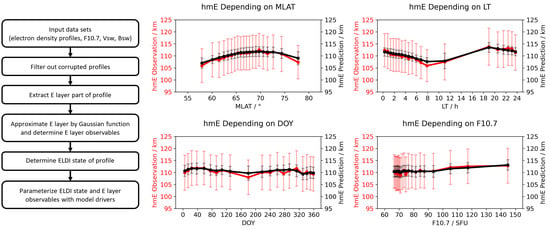
The propagation of HF radio waves also depends on the height of the reflecting layer. In this regard, below, we show the model equation (Equation (4)) and its corresponding coefficients (Table 3) for the peak height of the E layer. Figure 3 shows the related trends and the RMS values for the peak height. Since we found only a negligible variation of depending on the convection electric field magnitude in the initial trend analysis, this quantity is not considered as a driver in the model equation.
As expected, the height of the E layer is rather stable, varying between about 105 and 112 km for both hemispheres, with the RMS values being extended by about 7 km. These observations fit well with those of Cai et al. [10]. They found that at the EISCAT site (69.9°N), which is located inside the auroral oval for most of the time, was about 114 km for the majority of ELDI events. At the ESR site (78°N), which is mostly located outside the auroral oval, this value was around 108 km. The plots presenting the dependencies of on show a maximum in the latitude range between 65° and 70°, indicating the location of the auroral zone. Regarding the dependency on the local time, a minimum can be found around 8:00 to 12:00 LT. In contrast, the dependency on shows only a minor semiannual variation. Furthermore, we find that increases slightly for increasing . This effect could be explained by the higher amount of EUV irradiance and enhanced heating for increasing , which causes an expansion of the upper atmospheric layers in general. For both hemispheres, the range of the observed is largest depending on (north: 7.9 km, south: 6.4 km).
4.3. NEEM-W: Model for the E Layer Vertical Profile Width
As follows, we introduce the model equation (Equation (5)) and its related coefficients (Table 4) for the vertical profile width of the E layer. The corresponding trends and the RMS are given in Figure 4.
As we can see from the plots, the average width of the E layer generally varies between about 15 and 21 km for both hemispheres. This value range is also in the order of magnitude of the E layer thickness observed by Cai et al. [10], who defined this parameter in a similar way to our E layer profile width. They found that at the ESR site, the E layer thickness was about 17 km for most of the ELDI events, while it was about 23 km at the EISCAT site. These observed magnitude ranges are quite different from the sporadic E layer thickness of up to 2 km at mid-latitudes [11,12,13]. It is interesting to note that the trends show a decrease in for increasing geomagnetic latitudes. Furthermore, we see a slight enhancement of around local noon and with increasing solar activity. The dependency shows a minor semidiurnal variation. For both hemispheres, the range of the observed is largest depending on (north: 5.4 km, south: 4.6 km).
4.4. NEEM-P: Model for the ELDI Occurrence Probability %ELDI
As explained in Section 3.2.2, we divided the value ranges of the model drivers into intervals to compute the external model coefficients. On the one hand, the number of intervals of a considered driver and, thus, of the resulting data points must be high enough to adequately represent the curve formed by the base functions included in the associated model term. On the other hand, this number is limited to ensure that each interval key is assigned a sufficiently large amount of profiles to obtain a good resolution. Our initial trend analysis showed that for describing the dependency, a single Gaussian function is suitable. For describing the and dependencies, the superposition of two cosine functions is appropriate in each case. All the listed function terms can be sufficiently approximated by six points each. In comparison, the basically linear and dependencies can be described by three points each. This results in the following interval numbers for the model drivers: : 6, : 6, : 6, : 3, : 3. For the modeling dataset, we want to ensure a minimum resolution of 1% for fitting the model equation to the –model driver combinations of the keys. Hence, we set the threshold for the minimum number of assigned profiles required by a valid key to 100. Table 5 shows statistical information about the keys generated for both hemispheres. Thereafter, we give the model equation (Equation (6)) and its coefficients (Table 6).
Figure 5 shows the corresponding trends and RMS values for the model.
Considering the trends for both hemispheres, we see that the largest value is about 12%. Similar to , also shows a maximum between 65° and 70° , which fits well with the findings of Kamal et al. [8,9]. In the case of a reduced solar zenith angle, as for example around local noon or in local summer, is decreased, which matches the observations of Cai et al. [10] and Kamal et al. [8,9]. A decrease in is also visible for increased solar activity, which was likewise found previously by Kamal et al. [8,9]. These dependencies could be explained by the fact that both a small solar zenith angle and a high solar activity are associated with an increased amount of solar irradiance. This causes an enhanced ionization of the upper ionospheric layers, especially of the F2 layer, thereby hiding the ionization of the E layer produced by particle precipitation. In this way, the number of occurring ELDI events decreases. For an increasing convection electric field magnitude, we also see an increase in , which is in line with the findings for and was also observed by Kamal et al. [9]. For both hemispheres, the range of the observed is largest depending on (north: 9.1 %, south: 13.0 %).
5. Model Validation
In this section, we give the results of validating our models with the test dataset. In this regard, we again show trends for the original model observable values (red) and for those as predicted by our models (black). Furthermore, we show the resulting RMS and NRMS values and compare them with the corresponding values presented in Section 4 for the modeling dataset.
Figure 6 shows the results of validating our model NEEM-N with the test dataset.
For the Northern Hemisphere, we find an NRMS of 36.1% for the modeling dataset, while this value is slightly increased to 36.3% for the test dataset. For the Southern Hemisphere, the NRMS for the test dataset is 46.9%. This value is slightly lower than the NRMS for the modeling data set, which is 47.1%.
Figure 7 shows the results of validating our model NEEM-H with the test dataset.
When comparing the Northern Hemisphere NRMS results for the modeling dataset with those for the test dataset, we find that the NRMS is 6.1 and 6.2%, respectively. For the Southern Hemisphere, we have the same NRMS of 6.3% for both datasets.
Figure 8 shows the validation results for the model NEEM-W after applying it to the test dataset.
By comparing the NRMS results, we see that for the Northern Hemisphere, we have a value of 38.6% for the modeling dataset, while this value is slightly decreased to 38.5% for the test dataset. In the case of the Southern Hemisphere, the NRMS for the two datasets is 41.0 and 41.1%, respectively.
With a share of only 1/10th of the full electron density profile dataset, the test dataset is much smaller than the modeling dataset. Consequently, for the qualitative validation of the model, it was necessary to adjust the interval key formation in such a way that a sufficiently large number of valid keys remain. Therefore, we reduced the threshold for the minimum number of assigned profiles required by each valid key to 50, resulting in a resolution of 2%. In addition, we reduced the number of intervals to four for the model drivers , and . Table 7 shows the corresponding statistical information about the interval keys generated for both hemispheres.
In Figure 9, we show the results of validating our model NEEM-P with the test dataset.
Regarding the NRMS for the Northern Hemisphere, we see a minor increase from 56.5% for the modeling dataset to 57.4% for the test dataset. For the Southern Hemisphere, we observe an increase from 58.7 to 60.3%.
It is interesting to note that for both the modeling dataset (Section 4) and the test dataset (Section 5), the Southern Hemisphere always shows a higher RMS deviation between the observation and the prediction than the Northern Hemisphere. Since we have chosen identical model equations for both hemispheres in all the cases, this effect could be due to a hemispherical asymmetry, which includes many aspects [25,26]. Consequently, further investigations are necessary to find out the exact causes of this effect.
6. Conclusions
In this paper, for the first time, we present the empirical Neustrelitz ELDI Event Model (NEEM), which climatologically describes the variation of the E layer dominated ionosphere (ELDI) for the high latitude regions of both hemispheres. NEEM depends on key model drivers. These are the geomagnetic latitude, day of year, local time, solar activity and convection electric field. The model is based on more than two million vertical electron density profiles covering more than one solar cycle from April 2006 to December 2018. The profiles were obtained from ionospheric GPS radio occultation observations on board the COSMIC/FORMOSAT-3 mission. NEEM consists of four submodels. Each submodel is defined by a parametric function equation, which is multiplicatively composed of several terms, one for each driver. The individual submodels NEEM-N, NEEM-H, NEEM-W and NEEM-P describe the peak density, the corresponding height and the width of the vertical E layer electron density profile, as well as the occurrence probability of the ELDI, respectively. The normalized root mean square deviation (NRMS) between the original and the predicted model observables yields similar values across both datasets and both hemispheres. For NEEM-N, we obtain an NRMS varying between 36.1 and 47.1%, and for NEEM-H between 6.1 and 6.3%. In the case of NEEM-W, the NRMS varies between 38.5 and 41.1%, whereas it varies between 56.5 and 60.3% for NEEM-P. In summary, the proposed NEEM represents a promising initial modeling approach for describing the occurrence probability of ELDI events, as well as the associated impact on the E-layer. As such, it paves the way for future prediction of the ELDI and its properties in applications, especially from the fields of terrestrial and space-based telecommunications and navigation. Nevertheless, several possibilities exist to improve NEEM. For example, increasing the size of the modeling dataset could lead to better statistics of the model observables and, thereby, increase the quality of the estimated coefficients. As with other models previously developed in Neustrelitz, the conversion of geographic into geomagnetic coordinates is based on the dipole magnetic field model. An alternative conversion using the IGRF model instead would cause more precise geomagnetic coordinates and, thus, improve the observed dependencies, especially on the geomagnetic latitude. Furthermore, by increasing the number of base functions contained in the individual model terms, the submodels would have more degrees of freedom available to adequately approximate the observed dependencies. Since NEEM is a climatological model that describes the averaged response of the ELDI to the drivers, the reliability to estimate the occurrence of individual ELDI events, often closely related to perturbation induced particle precipitation, is limited. Consequently, the results could certainly be further improved when considering the time delay between the observed solar wind parameters used as model drivers in this study and the magnetospheric–ionospheric–thermospheric response. This is a challenging task that will be addressed in future work.
Author Contributions
Conceptualization, S.K., N.J. and M.M.H.; methodology, S.K., N.J. and M.M.H.; software, S.K.; formal analysis, S.K., N.J. and M.M.H.; visualization, S.K.; writing—original draft preparation, S.K.; writing—review and editing, S.K., N.J., M.M.H. and J.W.; supervision, N.J. and M.M.H.; funding acquisition, M.M.H. All authors have read and agreed to the published version of the manuscript.
Funding
This research was funded by the German Research Foundation (DFG) under Grant No. HO 6136/1-1.
Acknowledgments
We thank the international team of the COSMIC/FORMOSAT-3 satellite mission for operating the satellites and the COSMIC Data Analysis and Archive Center for providing the derived observation data. We gratefully acknowledge the Space Physics Data Facility of the Goddard Space Flight Center for providing the observation data of the geophysical quantities used as the basis for our investigations in the present work.
Conflicts of Interest
The authors declare no conflict of interest. The funders had no role in the design of the study; in the collection, analyses, or interpretation of data; in the writing of the manuscript, or in the decision to publish the results.
References
- Davies, K. Ionospheric Radio; The Institution of Engineering and Technology: London, UK, 1990; ISBN 978-0863411861. [Google Scholar]
- Bates, H.F.; Hunsucker, D. Quiet and disturbed electron density profiles in the auroral zone ionosphere. Radio Sci. 1974, 9, 455–467. [Google Scholar] [CrossRef]
- Mayer, C.; Jakowski, N. Enhanced E-layer ionization in the auroral zones observed by radio occultation measurements onboard CHAMP and Formosat-3/COSMIC. Ann. Geophys. 2009, 27, 1207–1212. [Google Scholar] [CrossRef]
- Crowley, G.; Carlson, H.C.; Basu, S.; Denig, W.F.; Buchau, J.; Reinisch, B.W. The dynamic ionospheric polar hole. Radio Sci. 1993, 28, 401–413. [Google Scholar] [CrossRef]
- Benson, R.F.; Grebowsky, J.M. Extremely low ionospheric peak altitudes in the polar hole region. Radio Sci. 2001, 36, 277–285. [Google Scholar] [CrossRef] [Green Version]
- Rodger, A. The mid-latitude trough—Revisited. In Midlatitude Ionospheric Dynamics and Disturbances; Kintner, P.M., Coster, A.J., Fuller-Rowell, T., Mannucci, A.J., Mendillo, M., Heelis, R., Eds.; American Geophysical Union: Washington, DC, USA, 2008; Volume 181, pp. 25–33. [Google Scholar] [CrossRef]
- Aa, E.; Zou, S.; Erickson, P.J.; Zhang, S.-R.; Liu, S. Statistical analysis of the main ionospheric trough using swarm in situ measurements. J. Geophys. Res. Space Phys. 2020, 125, e2019JA027583. [Google Scholar] [CrossRef]
- Kamal, S.; Jakowski, N.; Hoque, M.M.; Wickert, J. Evaluation of E layer dominated ionosphere events using COSMIC/FORMOSAT-3 and CHAMP ionospheric radio occultation data. Remote Sens. 2020, 12, 333. [Google Scholar] [CrossRef] [Green Version]
- Kamal, S.; Jakowski, N.; Hoque, M.M.; Wickert, J.E. Layer dominated ionosphere occurrences as a function of geophysical and space weather conditions. Remote Sens. 2020, 12, 4109. [Google Scholar] [CrossRef]
- Cai, H.; Li, F.; Shen, G.; Zhan, W.; Zhou, K.; McCrea, I.W.; Ma, S. E layer dominated ionosphere observed by EISCAT/ESR radars during solar minimum. Ann. Geophys. 2014, 32, 1223–1231. [Google Scholar] [CrossRef]
- Kirkwood, S.; Nilsson, H. High-latitude sporadic-E and other thin layers—The role of magnetospheric electric fields. Space Sci. Rev. 2000, 91, 579–613. [Google Scholar] [CrossRef]
- Wu, D.L.; Ao, C.O.; Hajj, G.A.; de la Torre Juarez, M.; Mannucci, A.J. Sporadic E morphology from GPS-CHAMP radio occultation. J. Geophys. Res. 2005, 110, A01306. [Google Scholar] [CrossRef] [Green Version]
- Arras, C.; Wickert, J. Estimation of ionospheric sporadic E intensities from GPS radio occultation. J. Atmos. Sol. Terr. Phys. 2018, 171, 60–63. [Google Scholar] [CrossRef]
- Rocken, C.; Kuo, Y.-H.; Schreiner, W.S.; Hunt, D.; Sokolovskiy, S.; McCormick, C. COSMIC system description. Terr. Atmos. Ocean. Sci. 2000, 11, 21–52. [Google Scholar] [CrossRef] [Green Version]
- Liou, Y.-A.; Pavelyev, A.G.; Liu, S.-F.; Pavelyev, A.A.; Yen, N.; Huang, C.-Y.; Fong, C.-J. FORMOSAT-3/COSMIC GPS radio occultation mission: Preliminary results. IEEE Trans. Geosci. Remote Sens. 2007, 45, 3813–3826. [Google Scholar] [CrossRef]
- Anthes, R.A.; Bernhardt, P.A.; Chen, Y.; Cucurull, L.; Dymond, K.F.; Ector, D.; Healy, S.B.; Ho, S.-P.; Hunt, D.C.; Kuo, Y.-H.; et al. The COSMIC/FORMOSAT-3 mission: Early results. Bull. Am. Meteorol. Soc. 2008, 89, 313–333. [Google Scholar] [CrossRef]
- Reigber, C.; Lühr, H.; Schwintzer, P.; Wickert, J. Earth Observation with CHAMP: Results from Three Years in Orbit; Springer: Berlin, Germany, 2005; ISBN 978-3-540-26800-0. [Google Scholar]
- Mannucci, A.J.; Tsurutani, B.T.; Verkhoglyadova, O.; Komjathy, A.; Pi, X. Use of radio occultation to probe the high-latitude ionosphere. Atmos. Meas. Tech. 2015, 8, 2789–2800. [Google Scholar] [CrossRef] [Green Version]
- Jakowski, N.; Hoque, M.M.; Mayer, C. A new global TEC model for estimating transionospheric radio wave propagation errors. J. Geod. 2011, 85, 965–974. [Google Scholar] [CrossRef]
- Hoque, M.M.; Jakowski, N. A new global empirical NmF2 model for operational use in radio systems. Radio Sci. 2011, 46, 1–13. [Google Scholar] [CrossRef]
- Hoque, M.M.; Jakowski, N. A new global model for the ionospheric F2 peak height for radio wave propagation. Ann. Geophys. 2012, 30, 797–809. [Google Scholar] [CrossRef] [Green Version]
- CDAAC. COSMIC Data Analysis and Archive Center. Available online: https://cdaac-www.cosmic.ucar.edu/ (accessed on 9 June 2021).
- SPDF. OMNIWeb Service. Available online: https://omniweb.gsfc.nasa.gov/ (accessed on 9 June 2021).
- Kelley, M.C. The Earth’s Ionosphere: Plasma Physics and Electrodynamics, 2nd ed.; Academic Press: Cambridge, MA, USA, 2009; Volume 96, ISBN 978-0120884254. [Google Scholar]
- Förster, M.; Haaland, S. Interhemispheric differences in ionospheric convection: Cluster EDI observations revisited. J. Geophys. Res. Space Phys. 2015, 120, 5805–5823. [Google Scholar] [CrossRef] [Green Version]
- Laundal, K.M.; Cnossen, I.; Milan, S.E.; Haaland, S.E.; Coxon, J.; Pedatella, N.M.; Förster, M.; Reistad, J.P. North–South Asymmetries in Earth’s Magnetic Field. Space Sci. Rev. 2017, 206, 225–257. [Google Scholar] [CrossRef] [Green Version]
Figure 1.
Flowchart of the data pre-processing steps.

Figure 2.
Observed (red) and predicted (black) NmE trends for the modeling dataset. Left column: Northern Hemisphere. Right column: Southern Hemisphere. Last row: root mean square deviation (RMS) and normalized RMS (NRMS) between observation and prediction.
Figure 2.
Observed (red) and predicted (black) NmE trends for the modeling dataset. Left column: Northern Hemisphere. Right column: Southern Hemisphere. Last row: root mean square deviation (RMS) and normalized RMS (NRMS) between observation and prediction.

Figure 3.
Observed (red) and predicted (black) hmE trends for the modeling dataset. Left column: Northern Hemisphere. Right column: Southern Hemisphere. Last row: RMS and NRMS deviation between observation and prediction.
Figure 3.
Observed (red) and predicted (black) hmE trends for the modeling dataset. Left column: Northern Hemisphere. Right column: Southern Hemisphere. Last row: RMS and NRMS deviation between observation and prediction.

Figure 4.
Observed (red) and predicted (black) wvE trends for the modeling dataset. Left column: Northern Hemisphere. Right column: Southern Hemisphere. Last row: RMS and NRMS deviation between observation and prediction.
Figure 4.
Observed (red) and predicted (black) wvE trends for the modeling dataset. Left column: Northern Hemisphere. Right column: Southern Hemisphere. Last row: RMS and NRMS deviation between observation and prediction.

Figure 5.
Observed (red) and predicted (black) %ELDI trends for the modeling dataset. (Left) Northern Hemisphere. (Right) Southern Hemisphere. Last row: RMS and NRMS deviation between observation and prediction.
Figure 5.
Observed (red) and predicted (black) %ELDI trends for the modeling dataset. (Left) Northern Hemisphere. (Right) Southern Hemisphere. Last row: RMS and NRMS deviation between observation and prediction.

Figure 6.
Observed (red) and predicted (black) NmE trends for the test dataset. (Left) Northern Hemisphere. (Right) Southern Hemisphere. Last row: RMS and NRMS deviation between observation and prediction.
Figure 6.
Observed (red) and predicted (black) NmE trends for the test dataset. (Left) Northern Hemisphere. (Right) Southern Hemisphere. Last row: RMS and NRMS deviation between observation and prediction.

Figure 7.
Observed (red) and predicted (black) hmE trends for the test dataset. (Left) Northern Hemisphere. (Right) Southern Hemisphere. Last row: RMS and NRMS deviation between observation and prediction.
Figure 7.
Observed (red) and predicted (black) hmE trends for the test dataset. (Left) Northern Hemisphere. (Right) Southern Hemisphere. Last row: RMS and NRMS deviation between observation and prediction.

Figure 8.
Observed (red) and predicted (black) wvE trends for the test dataset. (Left) Northern Hemisphere. (Right) Southern Hemisphere. Last row: RMS and NRMS deviation between observation and prediction.
Figure 8.
Observed (red) and predicted (black) wvE trends for the test dataset. (Left) Northern Hemisphere. (Right) Southern Hemisphere. Last row: RMS and NRMS deviation between observation and prediction.

Figure 9.
Observed (red) and predicted (black) %ELDI trends for the test dataset. (Left) Northern Hemisphere. (Right) Southern Hemisphere. Last row: RMS and NRMS deviation between observation and prediction.
Figure 9.
Observed (red) and predicted (black) %ELDI trends for the test dataset. (Left) Northern Hemisphere. (Right) Southern Hemisphere. Last row: RMS and NRMS deviation between observation and prediction.


Table 1.
Example interval division for the model drivers LT, DOY and F10.7.
| Interval Index | LT | DOY | F10.7 |
|---|---|---|---|
| 1 | [0.0–12.0) | [1–122] | [60–90) |
| 2 | [12.0–24.0) | [123–244] | [90–160) |
| 3 | [245–366] | [160–250] |
Table 2.
Coefficients of the E layer peak electron density (NmE) model for the Northern and Southern Hemispheres.
Table 2.
Coefficients of the E layer peak electron density (NmE) model for the Northern and Southern Hemispheres.
| NmE Model Coefficients North | NmE Model Coefficients South | ||||||||||
|---|---|---|---|---|---|---|---|---|---|---|---|
| Internal | External | Internal | External | ||||||||
| MLAT0 | = | 67.49° | c1 | = | 1.07 × 10⁻¹ | MLAT0 | = | −69.03° | c1 | = | 6.00 × 101 |
| σMLAT | = | 3.39° | c2 | = | −8.01 × 10⁻² | σMLAT | = | 377.96° | c2 | = | 1.63 × 10⁻² |
| LTD | = | 2.94 h | c3 | = | 6.58 × 10⁻² | LTD | = | 6.36 h | c3 | = | 5.80 × 10⁻² |
| LTSD | = | −2.36 h | c4 | = | 1.92 × 10⁻¹ | LTSD | = | −1.09 h | c4 | = | −2.50 × 10⁻¹ |
| DOYA | = | 165.58 d | c5 | = | −6.08 × 10⁻³ | DOYA | = | 166.77 d | c5 | = | 2.45 × 10⁻² |
| DOYSA | = | −113.12 d | c6 | = | 7.83 × 10⁻³ | DOYSA | = | −70.53 d | c6 | = | −1.07 × 10³ |
| c7 | = | 3.80 × 100 | c7 | = | −7.84 × 10⁻⁷ | ||||||
| c8 | = | 8.20 × 10⁴ | c8 | = | −2.19 × 10⁻² | ||||||
Table 3.
Coefficients of the E layer peak height (hmE) model for the Northern and Southern Hemispheres.
Table 3.
Coefficients of the E layer peak height (hmE) model for the Northern and Southern Hemispheres.
| hmE Model Coefficients North | hmE Model Coefficients South | ||||||||||
|---|---|---|---|---|---|---|---|---|---|---|---|
| Internal | External | Internal | External | ||||||||
| MLAT0 | = | 69.15° | c1 | = | 1.16 × 10⁻¹ | MLAT0 | = | −69.41° | c1 | = | −1.01 × 100 |
| σMLAT | = | 10.82° | c2 | = | 2.73 × 10⁻² | σMLAT | = | 569.19° | c2 | = | 2.12 × 10⁻² |
| LTD | = | −3.71 h | c3 | = | −7.94 × 10⁻³ | LTD | = | −1.12 h | c3 | = | 2.08 × 10⁻³ |
| LTSD | = | −1.79 h | c4 | = | −7.22 × 10⁻³ | LTSD | = | −2.27 h | c4 | = | −1.78 × 10⁻⁴ |
| DOYA | = | −171.11 d | c5 | = | 4.33 × 10⁻³ | DOYA | = | −175.39 d | c5 | = | 5.07 × 10⁻³ |
| DOYSA | = | −110.35 d | c6 | = | 3.25 × 10⁻² | DOYSA | = | −90.90 d | c6 | = | −3.33 × 100 |
| c7 | = | 9.71 × 101 | c7 | = | −1.41 × 10⁴ | ||||||
Table 4.
Coefficients of the E layer vertical profile width (wvE) model for the Northern and Southern Hemispheres.
Table 4.
Coefficients of the E layer vertical profile width (wvE) model for the Northern and Southern Hemispheres.
| wvE Model Coefficients North | wvE Model Coefficients South | ||||||||||
|---|---|---|---|---|---|---|---|---|---|---|---|
| Internal | External | Internal | External | ||||||||
| MLAT0 | = | 58.03° | c1 | = | 2.84 × 10⁻¹ | MLAT0 | = | −57.66° | c1 | = | 2.27 × 10⁻¹ |
| σMLAT | = | 4.55° | c2 | = | 1.03 × 10⁻¹ | σMLAT | = | 2.53° | c2 | = | 8.57 × 10⁻² |
| LTD | = | 11.70 h | c3 | = | −2.68 × 10⁻² | LTD | = | −11.15 h | c3 | = | 4.39 × 10⁻³ |
| LTSD | = | 4.87 h | c4 | = | 7.44 × 10⁻³ | LTSD | = | −6.24 h | c4 | = | −2.96 × 10⁻⁴ |
| DOYA | = | −107.25 d | c5 | = | 1.36 × 10⁻² | DOYA | = | 177.46 d | c5 | = | 3.41 × 10⁻² |
| DOYSA | = | −81.82 d | c6 | = | 4.02 × 10⁻² | DOYSA | = | −80.45 d | c6 | = | 3.36 × 10⁻² |
| c7 | = | 1.45 × 101 | c7 | = | 1.49 × 101 | ||||||
Table 5.
Statistical information about the interval keys of the modeling dataset for the Northern and Southern Hemispheres.
Table 5.
Statistical information about the interval keys of the modeling dataset for the Northern and Southern Hemispheres.
| Quantity | North | South |
|---|---|---|
| Mathematically possible number of keys | 1944 | 1944 |
| Number of keys with less than 100 profiles | 257 | 264 |
| Number of keys used for fitting | 1687 | 1680 |
| Minimum number of profiles per key | 100 | 100 |
| Maximum number of profiles per key | 468 | 437 |
Table 6.
Coefficients of the ELDI occurrence probability (%ELDI) model for the Northern and Southern Hemispheres.
Table 6.
Coefficients of the ELDI occurrence probability (%ELDI) model for the Northern and Southern Hemispheres.
| %ELDI Model Coefficients North | %ELDI Model Coefficients South | ||||||||||
|---|---|---|---|---|---|---|---|---|---|---|---|
| Internal | External | Internal | External | ||||||||
| MLAT0 | = | 68.25° | c1 | = | 8.38 × 100 | MLAT0 | = | −70.33° | c1 | = | −3.79 × 100 |
| σMLAT | = | 5.35° | c2 | = | 9.78 × 10⁻¹ | σMLAT | = | 10.50° | c2 | = | 8.23 × 10⁻¹ |
| LTD | = | 1.77 h | c3 | = | 2.96 × 10⁻² | LTD | = | 1.66 h | c3 | = | 3.40 × 10⁻² |
| LTSD | = | 2.21 h | c4 | = | −5.51 × 10⁻¹ | LTSD | = | 2.81 h | c4 | = | 7.82 × 10⁻¹ |
| DOYA | = | 169.43 d | c5 | = | 4.10 × 10⁻² | DOYA | = | 171.54 d | c5 | = | −6.13 × 10⁻² |
| DOYSA | = | −75.93 d | c6 | = | −6.42 × 10⁻³ | DOYSA | = | −86.53 d | c6 | = | −5.29 × 10⁻³ |
| c7 | = | 9.64 × 10⁻⁴ | c7 | = | −2.22 × 10⁻³ | ||||||
| c8 | = | 1.53 × 100 | c8 | = | −4.89 × 100 | ||||||
Table 7.
Statistical information about the interval keys of the test dataset for the Northern and Southern Hemispheres.
Table 7.
Statistical information about the interval keys of the test dataset for the Northern and Southern Hemispheres.
| Quantity | North | South |
|---|---|---|
| Mathematically possible number of keys | 576 | 576 |
| Number of keys with less than 50 profiles | 118 | 120 |
| Number of keys used for fitting | 458 | 456 |
| Minimum number of profiles per key | 50 | 50 |
| Maximum number of profiles per key | 131 | 130 |
Publisher’s Note: MDPI stays neutral with regard to jurisdictional claims in published maps and institutional affiliations. |
© 2021 by the authors. Licensee MDPI, Basel, Switzerland. This article is an open access article distributed under the terms and conditions of the Creative Commons Attribution (CC BY) license (https://creativecommons.org/licenses/by/4.0/).
Share and Cite
MDPI and ACS Style
Kamal, S.; Jakowski, N.; Hoque, M.M.; Wickert, J. A High Latitude Model for the E Layer Dominated Ionosphere. Remote Sens. 2021, 13, 3769. https://doi.org/10.3390/rs13183769
AMA Style
Kamal S, Jakowski N, Hoque MM, Wickert J. A High Latitude Model for the E Layer Dominated Ionosphere. Remote Sensing. 2021; 13(18):3769. https://doi.org/10.3390/rs13183769
Chicago/Turabian StyleKamal, Sumon, Norbert Jakowski, Mohammed Mainul Hoque, and Jens Wickert. 2021. "A High Latitude Model for the E Layer Dominated Ionosphere" Remote Sensing 13, no. 18: 3769. https://doi.org/10.3390/rs13183769
Note that from the first issue of 2016, this journal uses article numbers instead of page numbers. See further details here.