
Data Processing and Analysis of Eight-Beam Wind Profile Coherent Wind Measurement Lidar
by
Yuefeng Zhao
, 
Xiaojie Zhang
,
Yurong Zhang
,
Jinxin Ding
,
Kun Wang
,
Yuhou Gao
,
Runsong Su
and
Jing Fang
* Shandong Provincial Engineering and Technical Center of Light Manipulations & Shandong Provincial Key Laboratory of Optics and Photonic Device, School of Physics and Electronics, Shandong Normal University, Jinan 250014, China
*
Author to whom correspondence should be addressed.
Remote Sens. 2021, 13(18), 3549; https://doi.org/10.3390/rs13183549
Submission received: 29 June 2021
/
Revised: 2 September 2021
/
Accepted: 3 September 2021
/
Published: 7 September 2021
(This article belongs to the Special Issue Remote Sensing for Wind Speed and Ocean Currents)
Abstract
:Real-time measurement of atmospheric wind field parameters plays an important role in weather analysis and forecasting, including improving the efficiency of wind energy, particle tracking, boundary layer measurements, and airport security. In this study, a wind profile coherent wind Light Detection and Ranging (Lidar) measurement with a wavelength of 1.55 µm was developed and demonstrated based on the principle of eight-beam velocimetry. The wind speed information was retrieved, and vertical and horizontal profiles were calculated via power spectrum estimation of sampled echo signals through the measurement of the atmospheric wind field in Hefei for several consecutive days. The experimental results show that the wind profiles produced using different techniques are quite consistent and the standard error is less than 0.42 m/s compared with three-beam and five-beam wind measurements.
1. Introduction
The real-time measurements of the space atmospheric wind field not only have an impact on our daily lives but also have important applications in aerospace and civil engineering. Atmospheric wind field detection plays an important role in theoretical studies of the space atmosphere [1,2], wind farm performance evaluation [3,4], aviation meteorological safety [5], weather warnings [6], and environmental monitoring [7,8]. Early wind measuring devices included pilot balloons, high-altitude detectors, radio theodolite, and microwave radar. Due to the near detection range, low detection accuracy, and low spatial resolution, these methods cannot meet the actual demand. In 1964, Yeh and Cummius proposed a laser Doppler velocimetry method. In 1968, Browning and Wexler proposed a Doppler Light Detection and Ranging (Lidar) method using the Velocity Azimuth Display (VAD) [9] method to obtain wind profiles, in which the measurements of the radial velocity (also called the line-of-sight velocity) at different azimuth angles are combined to deduce the wind field components. In 1987, a team led by Kane et al. was the first to develop a 1.06-μm Nd: YAG coherent Doppler wind measurement Lidar. In 1998, Frehlich et al. introduced coherent Doppler Lidar measurements for boundary layer wind statistics [10]. Subsequently, Smith et al. [11], Kindler et al. [12], Peña et al. [13], and Wagner et al. [3] confirmed that wind Lidar is a very useful tool for the measurement of wind profiles. The concept of low-coherent Doppler meteorological wind Lidar with a continuous reference wave formed from part of the amplified radiation transistor-transistor-logic (TTL)-modulated Distributed Feedback (DFB)-laser, passing through the fiber ring delay, was proposed for the first time in 2011 [14]. Since then, all-fiber lasers with wavelengths of 1.5–1.6 µm have been used to improve the compactness and efficiency of coherent Lidar systems [2,15]. The data from Lidar wind measurements can be used to retrieve the wind turbulence parameters [16,17,18], identify weather conditions [19], and improve wind energy efficiency. Recently, wind profile Lidar has been demonstrated to have the advantages of high spatial and temporal resolutions, a high measurement accuracy, a long detection range, and strong anti-interference, and it has been widely used for the real-time detection of three-dimensional wind fields in the space atmosphere.
Wind profile Lidar mainly takes clear air as the detection object [20]. In the process of atmospheric propagation, the electromagnetic wave emitted by the laser telescopes is scattered due to the uneven refraction distribution caused by the atmospheric turbulence, and the backscattered energy is received by the wind profile radar [21,22]. The velocity component of the airflow along the direction of the radar beams is determined according to the Doppler effect, and the echo position is determined according to the roundtrip time of the echo signal. Wind profile Lidar has been used on ground-based [23], vehicle-based [24], and airborne platforms [25,26]. Banakh et al. demonstrated the possibility of using a two-beam method for wind profile estimation using pulsed coherent Doppler Lidar [27]. In previous studies, three-beam [28], five-beam, and six-beam Lidar [29] were more common. Because the echo signal is weak, the Lidar detection has been shown to be easily affected by various jamming issues. In the case of heavy rainfall, the Lidar will have a large amplitude interference spectrum peak in the echo power spectrum measured by one or more beam pointing, which will drown the echo signal, resulting in a large error in the wind measurement calculation results [30].
In this study, wind profile coherent wind measurement Lidar was used to transmit eight electromagnetic beams in different directions to detect the upper wind field by driving the exiting telescope with the rotation of the head [31,32]. The sampled echo signals were divided into distance gates matching the pulse width, and the corresponding power spectrum of the echo signal was obtained for each beam after signal processing. Then, the consistency checked method was used to eliminate the polluted echo signals in order to overcome the influence of the interference from the individual beams on the calculation results [33]. Therefore, compared with the three-beam and five-beam methods, the precision of the eight-beam coherent Lidar is higher.
2. Materials and Methods
2.1. Coherent Wind Measurement Lidar System of Wind Profile
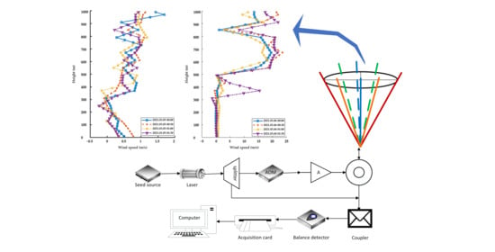
A diagram of the Lidar system is shown in Figure 1. The wind profile coherent wind measurement Lidar system is composed of a laser transmitting module and a receiving module. In this study, the transmitting and receiving modules of the telescope are integrated. In the laser transmitting module, the seed source is used to excite the laser to produce linearly polarized light with a central frequency of f0. The linearly polarized light is divided into a transmitting signal and a local oscillator (LO) signal after the beam splitter. The transmitted signal is modulated by an acousto-optic modulator into a pulse of light and generates a frequency shift of fm. Again, using the power amplifier, the final exit occurs after the circulator in the telescope. Due to the Doppler effect, the echo signal will produce a Doppler frequency shift of fd compared with the outgoing laser in the space atmospheric wind field [34]. The backscattered radiation from the aerosols entrained in the atmosphere is collected by the same telescope. At this time, the frequency of the backscattered echo signal received by the telescope is f0 + fm + fd. In the laser receiving module, the backscattered echo signal is coherently mixed with the LO signal, converted to intermediate frequency electrical signals with a frequency of fm + fd, and focused onto the balance detector. After sampling using the acquisition card, the echo signal is divided into numerous continuous distance gates according to the time sequence. In the digital processing circuit part, the power spectrum of the sampled echo signal is estimated, and the Doppler frequency shift is extracted. Finally, the wind speed information is retrieved through the Doppler frequency shift in the echo signal [35,36].
In this study, we used a pulsed Doppler Lidar system manufactured by Technovo Lidar High Tech Co. Ltd, Hefei, China (model KC-WL-2006 Lidar). The wind profile Lidar used the pulse trigger mode, and the laser wavelength was 1550 nm bands, which has the advantages of a high efficiency, being relatively safe for human eyes, and having a compact structure [37,38]. The all-fiber single-mode laser, which has a pulse width of 200 ns and a repetition frequency of 10 kHz, was used to measure the wind speed within a range of 3 km. The main parameters of the wind profile coherent wind measurement Lidar system are shown in Table 1.
2.2. Scanning Mode
In this study, the Lidar launched eight electromagnetic beams in different directions into the atmosphere by rotating the console to drive the telescope. The aerosol backscattered signals were received by the receiving telescope, and the echo signals were processed for high-altitude detection [39]. In order to synthesize the three-dimensional wind field in the space atmosphere, a series of beams with different directions were scanned via the Lidar to obtain the radial velocities in the different directions. The scanning mode of a Lidar system is divided according to the number of degrees of freedom. As shown in Figure 2, the beam orientation is defined in terms of the azimuth angle θ and the elevation angle φ. In the Vertical Azimuth Display (VAD) scanning technique, the measurement is made in at least three linearly independent directions, and when the wind fields are not uniform, the measurement errors will increase [40,41]. When more than three directions are used, extended tests under uniform and stable conditions can be carried out [21].
As shown in Figure 2, during the experiment, the Lidar operated in the VAD scanning mode for a period of 2.5 min. The elevation angle was fixed at 60°. The azimuth angle changed from 0° to 360°, with an angle step of 45°. Eight-beam wind measurement laser radars in a total of eight directions, namely, 45°, 90°, 135°, 180°, 225°, 270°, 315°, and 360°, were used. The radial spatial resolutions were set at 60 m in the range of 0–2.5 km [19].
2.3. Sample Collection and Data Processing Scheme
This study was conducted in Hefei, which is a typical prefecture-level city in eastern China. From 3 March to 6 March 2021, continuous observation of the wind field was carried out for 4 days. The experimental site was selected on the roof of the C4 Block in the Innovation Industrial Park (117.12°E, 31.85°N). The Lidar used was a 1550 nm eye-safe wind profile Lidar manufactured by Technovo Lidar High tech Co. Ltd. (model KC-WL-2006 Lidar). To prevent obstacles from blocking the laser beam, conical scanning using the probing beam at an elevation angle of φ = 60° was conducted in the experiment [29].
Strict quality control of the data was carried out [33]. The sounding data were checked for error points using a threshold, and the error points were removed. The ground and other noises were removed from the instantaneous data. These quality-controlled datasets were used in our analyses. A combined vertical profile of the magnitude and direction of the horizontal wind speed was obtained every half hour. First, the three-dimensional wind field of the space atmosphere was measured using the wind profile coherent wind measurement Lidar via fixed detection at regular times. In the observation process, the horizontal and vertical wind profiles were analyzed online to verify the consistency of the wind field. In addition, a Lidar with the same parameters produced by the same company was used in the comparison experiment (KC-WL-2003 and KC-WL-2004). A total of 192 groups of wind profiles were collected. In the following sections, representative data were selected for analysis.
In this study, the basic idea of coherent wind measurement Lidar data processing was to mix the received echo signal and to calculate the Doppler frequency shift through joint analysis of the time and frequency domains in order to synthesize the wind speed [42]. The time-domain analysis contains all of the information about the signal, which is more visual and can clearly illustrate the change in the signal. The frequency-domain analysis refers to the analysis of the time-domain signal through fast Fourier transform into the frequency domain, and the sampling of the time-domain signal follows the Nyquist sampling theorem. The specific data processing workflow is shown in Figure 3.
As shown in Figure 3, the data processing was conducted as follows. The binary data collected by the wind profile Lidar were divided into several continuous distance gates according to chronological order through the measurement of the atmospheric wind field in Hefei during several consecutive days. In the digital processing circuit, the power spectrum of the sampled echo signal was estimated, and the Doppler frequency shift was extracted through cumulative averaging of the pulses [43,44]. Finally, the wind speed information was retrieved through the Doppler frequency shift in the echo signal.
2.4. Range Gate Division of the Sampling Echo Signal
In this study, the pulse width was τ = 200 ns, the sampling frequency was fs = 1 GHz, and the number of sampling points at each radial distance was N = 400. To simplify the analysis, a section of effective data containing the peak value in the power spectrum was intercepted for analysis. The actual effective number of data points was Np = 112, and the corresponding range resolution was as follows:
The height of the blind area is related to the width of the mirror, i.e., the pulse width. In this study, the pulse width was τ = 200 ns; so, the blind area was B = 30 m. The single distance door diameter length L can be calculated using the following formula:
Therefore, the length of the nth distance from the door radial center is Ln = B + L × (n − 0.5), and the nth vertical center height of the distance gate is related to the wedge deflection angle θ. In this study, the wedge deflection angle was θ = 30°; so, the vertical center height of the nth distance gate was Ln times cosine of theta. For example, the center of the first distance gate was 60 m in the radial direction (Lr1) and 51.96 m in the vertical direction (Lv1).
The data collected by the eight-beam wind profile coherent wind measurement Lidar were divided into a number of continuous distance doors according to the time sequence. The eight-beam wind measurement Lidar has eight directions, namely, 45°, 90°, 135°, 180°, 225°, 270°, 315°, and 360°, a total of 65,536 power spectrum data points in each direction, and a total of 128 effective power spectrum data. Each range gate has 112 data points, that is, 1–14,336 points are effective data and the rest of the data are white noise data. As shown in Figure 4, the data in the first distance gate are noise data, and the corresponding sampling data points are points 1–112. The second and third distance gate data are the mirror data, and the corresponding sample data are points 113–336. The mirror data are formed by the reflection and refraction phenomenon of the telescope system itself. The data in the 4th to the 128th distance gates are valid data.
2.5. Methods of Wind Field Retrieval
The Doppler effect is used in velocity measurements of wind profile Lidar [35,42]. When there is a relative velocity between the target and the Lidar, the received echo signal will produce a frequency shift relative to the transmitted signal, which is the Doppler frequency shift. By extracting the Doppler frequency shift of the echo signal, the wind speed information can be retrieved.
The relationship between the Doppler frequency shift and the radial velocity is as follows:
where fd is the Doppler frequency shift, fr is the frequency of the echo signal, ft is the frequency of the output laser, Vr is the radial velocity of the target moving toward the radar, and λ is the laser wavelength. Therefore, the wind profile coherent wind measurement Lidar can effectively measure the space atmospheric wind field by checking the Doppler frequency shift of the echo signal. In this study, the frequency modulation Vm used in the wind profile coherent wind measurement Lidar was 80 MHz. When the wavelength was 1550 nm and the frequency modulation was 80 MHz, according to the Doppler frequency shift formula, the range of the measurable wind speed was ±62 m/s.
The atmospheric wind field is usually a function of space and time and has three-dimensional vector characteristics. Therefore, the measurement of the seasonal wind field at a certain position often requires the measurement of the three vector components of the wind field. However, a single-beam Lidar system can only measure the component of the wind vector along the line of sight of the laser beam. To accurately calculate the three-dimensional vector distribution of the wind field, at least three Lidar beams must pass the consistency test.
In this study, the sine-fitting method was used to retrieve the radial velocities from the VAD scanning. The sine-fitting method uses the azimuthal angular distribution of the radial velocity to find a fitted sine-curve function in the form described by Park et al., Augere et al. and Banakh et al. [45,46,47]. The following is an example of such an equation:
The three-dimensional wind vector V is calculated using Equation (7) with the same constants as in Equation (6):
Constants a, b, and θmax in Equation (6) are the offset, amplitude, and phase shift of the sine curve that best fits the VAD scan, respectively. θ and φ are the azimuth and elevation angle of the lidar beam, respectively. The horizontal wind direction γ is expressed as follows:
2.6. Calculation of the Wind Profile Lidar’s Carrier-to-Noise Ratio
The carrier-to-noise ratio (CNR) is an important index used to detect the performance of Lidar. The CNR directly determines the Lidar detection height. The CNR is dependent on both the instrument and the atmospheric variabilities within the resolution volume. In the radar system, the carrier-to-noise ratio refers to the ratio of the under modulated echo signal to the noise power. The accuracy of the velocity estimation is mainly determined by the CNR [48], that is, the carrier-to-noise ratio can be expressed as
where Ps is the power of the unmodulated echo signal, and Pn is the noise power. For each range-gate signal, subtract (para minus) the base noise signal of the first range-gate, and add the mean value of the base noise, and the resulting spectrum will be a flat base spectrum as shown in Figure 5. Then, find the maximum value of the power spectrum after denoising, and find the first point with a different downward trend on both sides successively (Figure 5). Divide the area of the red part by the area of the entire purple part, and the result is the CNR. In this paper, a threshold technique based on the CNR was applied to verify the validity of the data. The manufacturer of the Stream Line Doppler Lidar suggests using a threshold signal-to-noise ratio (SNR) of −18.2 dB (0.015) [49].
3. Results and Discussion
3.1. Error Analysis of the Three-Dimensional Wind Field Measurements
The wind profile Lidar is often interfered with by various noises during the detection process, which affects the spectral data. The environmental pollution sources of the spectral data include precipitation pollution, ground object clutter, and electromagnetic interference. Determining an accurate wind profile, especially at higher heights, is a challenging task due to these factors. Compared with clear-air turbulence, precipitation particles are strong scattering targets; so, the power spectrum within the range gate exhibits double peaks or even multiple peaks [50]. Cluttering, i.e., echoes, is produced by the presence of nearby stationary and slow-moving terrestrial targets such as trees and buildings. It presents as symmetrically placed low-frequency Doppler components around a frequency of 0 Hz [51,52]. Under the influence of radio signals in the environment surrounding the radar, narrow and sharp salt and pepper noise caused by the electromagnetic interference will appear in the power spectrum, which has a certain influence on the wind measurements. Due to the nature of the coherent detection, the main noise in the coherent Lidar system is proportional to the local oscillator power, such as the relative intensity noise; while the noise sources independent of the local oscillator power can be ignored [53]. In actual studies, it has been demonstrated that the maximum height that the radar system can detect is about 2.5 km after noise reduction processing; so, it can only extract 50 echo signals around the distance gate.
Figure 6 shows the power spectrum graph corresponding to the fourth range gate after Gaussian fitting. It can be seen from the graph that there are differences in the amplitude and frequency corresponding to the highest peak of the echo signal of the beam in different directions. The amplitude of the echo signal indicates the strength of the echo signal. In a certain amplitude range, it has no effect on the extraction of the Doppler frequency shift. After coherent beat demodulation, the difference between the corresponding frequencies of the highest peak of the echo signal directly reflects the magnitude of the Doppler frequency shift corresponding to the beam in the different directions, and this difference ultimately affects the magnitude and direction of the radial wind speed of the beam in the different directions.
3.2. Results of the Three-Dimensional Wind Field Measurements
Figure 7 shows the atmospheric vertical wind component information below 1 km observed in the Hefei area from 5 March to 6 March 2021. The horizontal coordinate represents the wind speed, and the vertical coordinate represents the height. Each profile in this figure shows the wind profile retrieved from the Lidar measurements for one scan (2 min) every half hour. It can be seen from Figure 7 that the wind speed did not change significantly below 300 m on 6 March and the average vertical wind speed was about 0.33 m/s. A low-level wind shear occurred below 400 m at 01:30 a.m. due to the turbulence of the low altitude upswing. As shown in Figure 7, the vertical wind direction diagram can more directly illustrate the drastic changes in the wind speed and direction with height perpendicular to the direction of the landmark.
The profiles from four consecutive Lidar volume scans (Figure 8) demonstrate the severe variations in the wind speed and direction with height, which may have been caused by turbulent changes before dawn. Each panel of this figure shows the wind profiles retrieved from Lidar measurements for one scan (2 min) every half hour. Taking into account that these measurements were conducted at a strongly stable stratification, we can assume that the variations in wind profiles for 1 h were most likely caused by the nonstationary process (mesoscale process) than by small-scale turbulence. It can be seen that the wind speed and direction changes were not significant (below 300 m), and the mean horizontal wind speed below 300 m was 11.4 m/s. An important feature of the VAD scanning Lidar analysis is the ability to provide accurate profiles in a short observation time compared with other radar products.
The experimental results show that the accuracies of the wind speed and direction measurements of the KC-WL-2006 Lidar are better than 0.2 m/s and 3°, respectively. The wind vectors were retrieved from eight radial wind velocity directions via the sine-fitting method. Thus, the eight-beam method partly overcomes the significant probe volume averaging problem, which is otherwise observed when using the VAD method. Compared with previous techniques, the eight-beam method has a higher wind measurement accuracy and the wind profile is smoother and no longer exhibits an obvious step shape. It has the capacity to detect the horizontal and vertical wind fields and to obtain large-scale, high-precision, high-resolution three-dimensional wind field data in real-time, which can be used for atmospheric boundary layer observations, wind field and flux observations and analysis, and aerosol spatial and temporal distribution analysis.
3.3. Contrast Observations
Generally, a set of radial velocity measurements are combined with appropriate assumptions to extract useful information for wind field analysis, such as the wind speeds and directions [21]. A 30-min average profile of the wind vector was calculated based on the assumption of a horizontally homogeneous wind field. There is a degree of correlation between the symmetrical beam measurements [41,54].
The combined calculation of the wind field using the eight-beam points can overcome the pollution of the individual beam effectively and can improve the quality of the calculated data. In order to verify the performance of the eight-beam wind profile coherent wind measurement Lidar system, a comparative experiment of wind measurement using wind profile Lidar was carried out successfully. Over 48 h of data were obtained for the entire comparison experiment. Figure 9 shows a comparison of the horizontal winds at 7:30 a.m. on 5 March 2021. The quality-controlled Lidar measurements were compared with independent reference data from two collocated operational Lidar wind profiles running in three-beam and five-beam Doppler beam swinging modes. The parameters of the instruments used for the three experiments were the same. The directions of the three-beam wind measurements were north (0°), east (90°), and vertical. The directions of the five-beam wind measurements were north (0°), east (90°), south (180°), west (270°), and vertical. During the experiment, an elevation angle of 60° and a range resolution of 30 m were used for the measurements. A combined vertical profile of the magnitude and direction of the horizontal wind speed was obtained every half hour. The main purpose of the experiment was to compare the magnitudes and directions of the horizontal wind fields measured using the three techniques in the same time and space domains under the same weather conditions.
As shown in Figure 9, the wind profiles obtained using the different techniques exhibit good consistency. Within the height range of 1 km, from 7:00 to 7:30 in the morning, the maximum values of the standard deviation of the magnitude and direction of the horizontal wind speed measured using the three instruments were 2.44 m/s and 43.15°, respectively, with average values of 0.42 m/s and 6.70°, respectively. These errors include the systematic measurement errors and the errors caused by atmospheric changes during the 30-min measurement period. At altitudes greater than 700 m, the difference in the wind speeds measured using the eight-beam and other techniques was observed, especially at altitudes of 800–1000 m.
The experimental results show that the standard error was less than 0.42 m/s compared with the results obtained from the three-beam and five-beam wind measurements. As can be seen from Figure 10, the absolute error varied with height. The average absolute error between the eight-beam and three-beam techniques was 0.34 m/s at heights of <300 m. The average absolute error between the eight-beam and five-beam techniques was −0.094 m/s at heights of <300 m. A positive number indicates a high wind speed measured by the eight-beam, and vice versa. At this time, the accuracy of the wind measurements was greatly affected by the cluttering near the ground objects. The average absolute error between the eight-beam and the three-beam techniques was 0.01 m/s below heights of 300–700 m. The average absolute error between the eight-beam and the five-beam techniques was 0.23 m/s below heights of 300–700 m. During this period, the influence of the near-ground cluttering decreased significantly, and the results obtained using the eight-beam technique are in good agreement with those obtained using the other techniques. Since the climatic conditions were relatively stable during the entire measurement period, these calculated variances in the data can serve as a reference for evaluating the measurement error of the system.
3.4. Calculation of the Wind Profile Lidar’s Carrier-to-Noise Ratio
Figure 11 shows the relationship between the CNR and the detection distance (Baud ratio) drawn according to the above calculation method. As can be seen from the figure, the CNR approximately decreases with increasing detection distance. This shows that the dynamic variation range of the echo signals is large and the amplitude of the echo signal decreases with the increasing detection distance. The wind profile coherent wind measurement Lidar system is a weak signal detection system. Under the condition that the detection distance is as long as possible to ensure the accuracy of extracting the wind field information, the weak signal is always the difficulty in coherent wind measurement Lidar.
4. Conclusions
In this study, we took advantage of the wind profile Lidar’s high spatial and temporal resolutions, high measurement accuracy, long-distance detection, and strong anti-interference characteristics to develop a method to measure the three-dimensional atmospheric wind speed field. In addition, by dividing the range gate to calculate the wind speed at different altitudes, the noise data and mirror data were limited to the first three range gates. Based on this, we proposed a method to calculate the CNR of the wind profile coherent wind measurement Lidar system. The experimental results show that the wind profiles obtained using the different techniques are quite consistent and the standard error is less than 0.42 m/s compared with the three-beam and five-beam wind measurements. In summary, based on an in-depth analysis of the power spectrum of the echo signal, the proposed method has good accuracy and provides robust atmospheric wind measurements.
Author Contributions
Conceptualization, Y.G. and R.S.; investigation, Y.Z. (Yurong Zhang), J.D. and K.W.; methodology, X.Z.; resources, Y.Z. (Yuefeng Zhao); supervision, J.F.; writing—original draft, X.Z.; writing—review and editing, Y.Z. (Yuefeng Zhao). All authors have read and agreed to the published version of the manuscript.
Funding
This research was funded by the Natural Science Foundation of Shandong Province, grant number ZR2020MA082 and Key Technology Research and Development Program of Shandong, grant number 2016GGX101016.
Conflicts of Interest
The authors declare no conflict of interest.
References
- Shangguan, M.; Xia, H.; Wang, C.; Qiu, J.; Shentu, G.; Zhang, Q.; Dou, X.; Pan, J.W. All-fiber upconversion high spectral resolution wind lidar using a Fabry-Perot interferometer. Opt. Express 2016, 24, 19322–19336. [Google Scholar] [CrossRef] [PubMed]
- Jiang, S.; Jiang, S.; Sun, D.S.; Han, Y.L.; Han, F.; Zhou, A.R.; Zheng, J. Performance of Continuous-wave Coherent Doppler Lidar for Wind Measurement. Curr. Opt. Photonics 2019, 3, 466–472. [Google Scholar]
- Wagner, R.; Courtney, M.; Gottschall, J.; Lindelow-Marsden, P. Accounting for the speed shear in wind turbine power performance measurement. Wind. Energy 2011, 14, 993–1004. [Google Scholar] [CrossRef] [Green Version]
- Bohme, G.S.; Fadigas, E.A.; Martinez, J.R.; Tassinari, C.E.M. Analysis of the Use of Remote Sensing Measurements for Developing Wind Power Projects. J. Sol. Energy Eng. 2019, 141, 041005. [Google Scholar] [CrossRef]
- Targ, R.; Kavaya, M.J.; Huffaker, R.M.; Bowles, R.L. Coherent lidar airborne windshear sensor: Performance evaluation. Appl. Opt. 1991, 30, 2013–2026. [Google Scholar] [CrossRef] [PubMed]
- Zhang, H.W.; Wu, S.H.; Wang, Q.C.; Liu, B.Y.; Yin, B.; Zhai, X.C. Airport low-level wind shear lidar observation at Beijing Capital International Airport. Infrared Phys. Technol. 2019, 96, 113–122. [Google Scholar] [CrossRef] [Green Version]
- Xia, H.Y.; Shentu, G.L.; Shangguan, M.J.; Xia, X.X.; Jia, X.D.; Wang, C.; Zhang, J.; Pelc, J.S.; Fejer, M.M.; Zhang, Q.; et al. Long-range micro-pulse aerosol lidar at 1.5 mu m with an upconversion single-photon detector. Opt. Lett. 2015, 40, 1579–1582. [Google Scholar] [CrossRef] [PubMed]
- Wang, X.; Cai, Y.J.; Wang, J.J.; Zhao, Y.F. Concentration monitoring of volatile organic compounds and ozone in Xi’an based on PTR-TOF-MS and differential absorption lidar. Atmos. Environ. 2021, 245, 12. [Google Scholar] [CrossRef]
- Xu, Q.; Nai, K.; Wei, L. Fitting VAD winds to aliased Doppler radial-velocity observations: A global minimization problem in the presence of multiple local minima. Q. J. R. Meteorol. Soc. 2010, 136, 451–461. [Google Scholar] [CrossRef]
- Frehlich, R.; Hannon, S.M.; Henderson, S.W. Coherent Doppler lidar measurements of wind field statistics. Bound.-Layer Meteorol. 1998, 86, 233–256. [Google Scholar] [CrossRef]
- Smith, D.A.; Harris, M.; Coffey, A.S.; Mikkelsen, T.; Jorgensen, H.E.; Mann, J.; Danielian, G. Wind lidar evaluation at the Danish wind test site in Hovsore. Wind Energy 2006, 9, 87–93. [Google Scholar] [CrossRef]
- Kindler, D.; Oldroyd, A.; Macaskill, A.; Finch, D. An eight month test campaign of the Qinetiq ZephIR system: Preliminary results. Meteorol. Z. 2007, 16, 479–489. [Google Scholar] [CrossRef]
- Pefia, A.; Hasager, C.B.; Gryning, S.E.; Courtney, M.; Antoniou, I.; Mikkelsen, T. Offshore Wind Profiling Using Light Detection and Ranging Measurements. Wind Energy 2009, 12, 105–124. [Google Scholar]
- Grishin, A.I.; Matvienko, G.G.; Polyakov, S.N. All-fiber wind low-coherent Doppler meteorological lidar. Prikl. Fiz. 2011, 4, 121–125. [Google Scholar]
- Zhou, P.; Wang, X.L.; Ma, Y.X.; Han, K.; Liu, Z.J. Stable all-fiber dual-wavelength thulium-doped fiber laser and its coherent beam combination. Laser Phys. 2011, 21, 184–187. [Google Scholar] [CrossRef]
- Banakh, V.A.; Smalikho, I.N.; Falits, A.V. Estimation of the height of the turbulent mixing layer from data of Doppler lidar measurements using conical scanning by a probe beam. Atmos. Meas. Tech. 2021, 14, 1511–1524. [Google Scholar] [CrossRef]
- Li, S.W.; Tse, K.T.; Weerasuriya, A.U.; Chan, P.W. Estimation of turbulence intensities under strong wind conditions via turbulent kinetic energy dissipation rates. J. Wind. Eng. Ind. Aerodyn. 2014, 131, 1–11. [Google Scholar] [CrossRef]
- Smalikho, I.N.; Banakh, V.A. Measurements of wind turbulence parameters by a conically scanning coherent Doppler lidar in the atmospheric boundary layer. Atmos. Meas. Tech. 2017, 10, 4191–4208. [Google Scholar] [CrossRef] [Green Version]
- Yuan, J.L.; Xia, H.Y.; Wei, T.W.; Wang, L.; Yue, B.; Wu, Y.B. Identifying cloud, precipitation, windshear, and turbulence by deep analysis of the power spectrum of coherent Doppler wind lidar. Opt. Express 2020, 28, 37406–37418. [Google Scholar] [CrossRef]
- Kameyama, S.; Ando, T.; Asaka, K.; Hirano, Y.; Wadaka, S. Compact all-fiber pulsed coherent Doppler lidar system for wind sensing. Appl. Opt. 2007, 46, 1953–1962. [Google Scholar] [CrossRef]
- Liu, Z.L.; Barlow, J.F.; Chan, P.W.; Fung, J.C.H.; Li, Y.G.; Ren, C.; Mak, H.W.L.; Ng, E.A. A Review of Progress and Applications of Pulsed Doppler Wind LiDARs. Remote Sens. 2019, 11, 2522. [Google Scholar] [CrossRef] [Green Version]
- Gao, J.; Gao, J.; Pan, J.; Wang, J.J.; Cai, Y.J.; Zhao, Y.F. Triple charge-coupled device cameras combined backscatter lidar for retrieving PM2.5 from aerosol extinction coefficient. Appl. Opt. 2020, 59, 10369–10379. [Google Scholar] [CrossRef] [PubMed]
- Dolfi-Bouteyre, A.; Canat, G.; Valla, M.; Augere, B.; Besson, C.; Goular, D.; Lombard, L.; Cariou, J.P.; Durecu, A.; Fleury, D.; et al. Pulsed 1.5-mu m LIDAR for Axial Aircraft Wake Vortex Detection Based on High-Brightness Large-Core Fiber Amplifier. Ieee J. Sel. Top. Quantum Electron. 2009, 15, 441–450. [Google Scholar] [CrossRef]
- Zhang, G.Z.; Li, J.; Wang, Y.; Liu, Z.S.; Chang, D.L.; Tian, J.H. Vehicle-mounted validations of a 1.55-mu m all-fiber continuous-wave coherent laser radar for measuring aircraft airspeed. Opt. Eng. 2019, 58, 9. [Google Scholar]
- Greco, S.; Emmitt, G.D.; DuVivier, A.; Hines, K.; Kavaya, M. Polar Winds: Airborne Doppler Wind Lidar Missions in the Arctic for Atmospheric Observations and Numerical Model Comparisons. Atmosphere 2020, 11, 1141. [Google Scholar] [CrossRef]
- Chouza, F.; Reitebuch, O.; Gross, S.; Rahm, S.; Freudenthaler, V.; Toledano, C.; Weinzierl, B. Retrieval of aerosol backscatter and extinction from airborne coherent Doppler wind lidar measurements. Atmos. Meas. Tech. 2015, 8, 2909–2926. [Google Scholar] [CrossRef] [Green Version]
- Banakh, V.A.; Smalikho, I.N.; Falits, A.V.; Gordeev, E.V.; Sukharev, A.A. Demonstration of the possibility of using a duo-beam method for wind profile estimation by pulsed coherent Doppler lidar. Russ. Phys. J. 2017, 60, 175–178. [Google Scholar]
- Prasad, N.S.; Mylapore, A.R. Three-beam aerosol backscatter correlation lidar for wind profiling. Opt. Eng. 2017, 56, 031222. [Google Scholar] [CrossRef]
- Sathe, A.; Mann, J.; Vasiljevic, N.; Lea, G.A. A six-beam method to measure turbulence statistics using ground-based wind lidars. Atmos. Meas. Tech. 2015, 8, 729–740. [Google Scholar] [CrossRef] [Green Version]
- Chumchean, S.; Sharma, A.; Seed, A. Radar rainfall error variance and its impact on radar rainfall calibration. Phys. Chem. Earth 2003, 28, 27–39. [Google Scholar] [CrossRef]
- Liu, H.T.; Wang, Z.Z.; Zhao, J.X.; Ma, J.J. Error Accumulation and Transfer Effects of the Retrieved Aerosol Backscattering Coefficient Caused by Lidar Ratios. Curr. Opt. Photonics 2018, 2, 119–124. [Google Scholar]
- Henderson, S.W.; Hale, C.P.; Magee, J.R.; Kavaya, M.J.; Huffaker, A.V. Eye-safe coherent laser radar system at 2.1 microm using Tm,Ho:YAG lasers. Opt. Lett. 1991, 16, 773–775. [Google Scholar] [CrossRef]
- Holleman, I. Quality control and verification of weather radar wind profiles. J. Atmos. Ocean. Technol. 2005, 22, 1541–1550. [Google Scholar] [CrossRef] [Green Version]
- Frehlich, R.; Kelley, N. Measurements of Wind and Turbulence Profiles With Scanning Doppler Lidar for Wind Energy Applications. IEEE J. Sel. Top. Appl. Earth Obs. Remote. Sens. 2008, 1, 42–47. [Google Scholar] [CrossRef]
- Kameyama, S.; Ando, T.; Asaka, K.; Hirano, Y.; Wadaka, S. Performance of Discrete-Fourier-Transform-Based Velocity Estimators for a Wind-Sensing Coherent Doppler Lidar System in the Kolmogorov Turbulence Regime. Ieee Trans. Geosci. Remote Sens. 2009, 47, 3560–3569. [Google Scholar] [CrossRef]
- Wu, S.H.; Liu, B.Y.; Liu, J.T.; Zhai, X.C.; Feng, C.Z.; Wang, G.N.; Zhang, H.W.; Yin, J.P.; Wang, X.T.; Li, R.Z. Wind turbine wake visualization and characteristics analysis by Doppler lidar. Opt. Express 2016, 24, A762–A780. [Google Scholar] [CrossRef]
- Shangguan, M.J.; Wang, C.; Xia, H.Y.; Shentu, G.L.; Dou, X.K.; Zhang, Q.; Pan, J.W. Brillouin optical time domain reflectometry for fast detection of dynamic strain incorporating double-edge technique. Opt. Commun. 2017, 398, 95–100. [Google Scholar] [CrossRef] [Green Version]
- Karlsson, C.J.; Olsson, F.A.A.; Letalick, D.; Harris, M. All-fiber multifunction continuous-wave coherent laser radar at 1.55 mu m for range, speed, vibration, and wind measurements. Appl. Opt. 2000, 39, 3716–3726. [Google Scholar] [CrossRef]
- Panne, U. Laser remote sensing. Trac-Trends Anal. Chem. 1998, 17, 491–500. [Google Scholar] [CrossRef]
- Liang, X.D. An integrating velocity-azimuth process single-Doppler radar wind retrieval method. J. Atmos. Ocean. Technol. 2007, 24, 658–665. [Google Scholar] [CrossRef]
- Teschke, G.; Lehmann, V. Mean wind vector estimation using the velocity-azimuth display (VAD) method: An explicit algebraic solution. Atmos. Meas. Tech. 2017, 10, 3265–3271. [Google Scholar] [CrossRef] [Green Version]
- Wang, C.; Xia, H.Y.; Liu, Y.P.; Lin, S.F.; Dou, X.K. Spatial resolution enhancement of coherent Doppler wind lidar using joint time-frequency analysis. Opt. Commun. 2018, 424, 48–53. [Google Scholar] [CrossRef]
- Akhmetianov, V.R.; Mishina, O.A. Processing of Wind Coherent Doppler Lidar Data on the Base of Gaussian Approximation Method. Izvestiya vysshikh uchebnykh zavedenii. Priborostroenie 2010, 53, 20–26. [Google Scholar]
- Beyon, J.Y.; Koch, G.J. Novel nonlinear adaptive Doppler-shift estimation technique for the coherent Doppler validation lidar. Opt. Eng. 2007, 46, 10. [Google Scholar]
- Park, S.J.; Kim, S.W.; Park, M.S.; Song, C.K. Measurement of Planetary Boundary Layer Winds with Scanning Doppler Lidar. Remote Sens. 2018, 10, 1261. [Google Scholar] [CrossRef] [Green Version]
- Augere, B.; Valla, M.; Durécu, A.; Dolfi-Bouteyre, A.; Goular, D.; Gustave, F.; Planchat, C.; Fleury, D.; Huet, T.; Besson, C. Three-Dimensional Wind Measurements with the Fibered Airborne Coherent Doppler Wind Lidar LIVE. Atmosphere 2019, 10, 549. [Google Scholar] [CrossRef] [Green Version]
- Banakh, V.A.; Brewer, A.; Pichugina, E.I.; Smalikho, I.N. Wind velocity and direction measurement with a coherent Doppler lidar under conditions of weak echo signal. Atmos. Oceanic. Opt. 2010, 23, 333–340. [Google Scholar] [CrossRef]
- Wang, C.; Xia, H.Y.; Shangguan, M.J.; Wu, Y.B.; Wang, L.; Zhao, L.J.; Qiu, J.W.; Zhang, R.J. 1.5 mu m polarization coherent lidar incorporating time-division multiplexing. Opt. Express 2017, 25, 20663–20674. [Google Scholar] [CrossRef] [Green Version]
- Liu, H.; Yuan, L.C.; Fan, C.H.; Liu, F.F.; Zhang, X.; Zhu, X.P.; Liu, J.Q.; Zhu, X.L.; Chen, W.B. Performance validation on an all-fiber 1.54-mu m pulsed coherent Doppler lidar for wind-profile measurement. Opt. Eng. 2020, 59, 11. [Google Scholar] [CrossRef] [Green Version]
- Schween, J.H.; Hirsikko, A.; Lohnert, U.; Crewell, S. Mixing-layer height retrieval with ceilometer and Doppler lidar: From case studies to long-term assessment. Atmos. Meas. Tech. 2014, 7, 3685–3704. [Google Scholar] [CrossRef] [Green Version]
- Hooper, D.A. Signal and noise level estimation for narrow spectral width returns observed by the Indian MST radar. Radio Sci. 1999, 34, 859–870. [Google Scholar] [CrossRef]
- Sinha, S.; Sarma, T.V.C.; Regeena, M.L. Estimation of Doppler Profile Using Multiparameter Cost Function Method. IEEE Trans. Geosci. Remote. Sens. 2017, 55, 932–942. [Google Scholar] [CrossRef]
- Harris, M.; Pearson, G.N.; Vaughan, J.M.; Letalick, D.; Karlsson, C. The role of laser coherence length in continuous-wave coherent laser radar. J. Mod. Opt. 1998, 45, 1567–1581. [Google Scholar] [CrossRef]
- Paeschke, E.; Leinweber, R.; Lehmann, V. An assessment of the performance of a 1.5 mu m Doppler lidar for operational vertical wind profiling based on a 1-year trial. Atmos. Meas. Tech. 2015, 8, 2251–2266. [Google Scholar] [CrossRef] [Green Version]
Figure 1.
Wind profile Lidar system.

Figure 2.
Schematic diagram of eight-beam coherent wind measurement Lidar.

Figure 3.
Data processing flowchart.

Figure 4.
Power spectrum of the raw data.

Figure 5.
The method of calculating the CNR of the range gate division of the Lidar.

Figure 6.
Beam frequency shift contrast diagram.

Figure 7.
Wind profiles obtained for two consecutive days in the vertical direction.

Figure 8.
Profiles of the horizontal wind speed and direction from 00:00 to 01:30 on 6 March 2021.

Figure 9.
Comparisons of the calculation results of the eight-beam check with the three-beam and five-beam wind measurements.
Figure 9.
Comparisons of the calculation results of the eight-beam check with the three-beam and five-beam wind measurements.

Figure 10.
Variation in the absolute deviation with height between the different beam measurements.

Figure 11.
The relationship between the CNR and the detection range.


Table 1.
Wind profile radar system parameters.
| Component | Qualification | Specification |
|---|---|---|
| Transmitter | Operating wavelength | 1550 nm |
| Pulse energy | 145 μJ | |
| Pulse repetition | 10 KHz | |
| Pulse width | 200 ns | |
| Transceiver | Laser mode | Pulse |
| Scan mode | Conical | |
| Elevation angle | 60° | |
| Start angle | 0° | |
| Step angle | 45° | |
| Data-Acquisition | Sampling frequency | 1 GHz |
| Sampling points | 150 | |
| Range resolution | 30 m | |
| Blind range | 30 m | |
| Gate number | 128 |
Publisher’s Note: MDPI stays neutral with regard to jurisdictional claims in published maps and institutional affiliations. |
© 2021 by the authors. Licensee MDPI, Basel, Switzerland. This article is an open access article distributed under the terms and conditions of the Creative Commons Attribution (CC BY) license (https://creativecommons.org/licenses/by/4.0/).
Share and Cite
MDPI and ACS Style
Zhao, Y.; Zhang, X.; Zhang, Y.; Ding, J.; Wang, K.; Gao, Y.; Su, R.; Fang, J. Data Processing and Analysis of Eight-Beam Wind Profile Coherent Wind Measurement Lidar. Remote Sens. 2021, 13, 3549. https://doi.org/10.3390/rs13183549
AMA Style
Zhao Y, Zhang X, Zhang Y, Ding J, Wang K, Gao Y, Su R, Fang J. Data Processing and Analysis of Eight-Beam Wind Profile Coherent Wind Measurement Lidar. Remote Sensing. 2021; 13(18):3549. https://doi.org/10.3390/rs13183549
Chicago/Turabian StyleZhao, Yuefeng, Xiaojie Zhang, Yurong Zhang, Jinxin Ding, Kun Wang, Yuhou Gao, Runsong Su, and Jing Fang. 2021. "Data Processing and Analysis of Eight-Beam Wind Profile Coherent Wind Measurement Lidar" Remote Sensing 13, no. 18: 3549. https://doi.org/10.3390/rs13183549
Note that from the first issue of 2016, this journal uses article numbers instead of page numbers. See further details here.