Evaluating Simulated RADARSAT Constellation Mission (RCM) Compact Polarimetry for Open-Water and Flooded-Vegetation Wetland Mapping

Canada Centre for Mapping and Earth Observation, Natural Resources Canada, 560 Rochester St, Ottawa, ON K1S 5K2, Canada
*
Author to whom correspondence should be addressed.
Remote Sens. 2020, 12(9), 1476; https://doi.org/10.3390/rs12091476
Submission received: 6 March 2020
/
Revised: 30 April 2020
/
Accepted: 2 May 2020
/
Published: 6 May 2020
(This article belongs to the Special Issue Wetland Landscape Change Mapping Using Remote Sensing)
Abstract
:When severe flooding occurs in Canada, the Emergency Geomatics Service (EGS) is tasked with creating and disseminating maps that depict flood extents in near real time. EGS flood mapping methods were created with efficiency and robustness in mind, to allow maps to be published quickly, and therefore have the potential to generate high-repeat water products that can enhance frequent wetland monitoring. The predominant imagery currently used is synthetic aperture radar (SAR) from RADARSAT-2 (R2). With the commissioning phase of the RADARSAT Constellation Mission (RCM) complete, the EGS is adapting its methods for use with this new source of SAR data. The introduction of RCM’s circular-transmit linear-receive (CTLR) beam mode provides the option to exploit compact polarimetric (CP) information not previously available with R2. The aim of this study was to determine the most effective CP parameters for use in mapping open water and flooded vegetation, using current EGS methodologies, and compare these products to those created by using R2 data. Nineteen quad-polarization R2 scenes selected from three regions containing wetlands prone to springtime flooding were used to create reference flood maps, using existing EGS tools. These scenes were then used to simulate 22 RCM CP parameters at different noise floors and spatial resolutions representative of the three RCM beam modes. Using multiple criteria, CP parameters were ranked in order of importance and entered into a stepwise classification procedure, for evaluation against reference R2 products. The top four CP parameters —m-chi-volume or m-delta-volume, RR intensity, Shannon Entropy intensity (SEi), and RV intensity—achieved a maximum agreement with baseline R2 products of upward of 98% across all 19 scenes and three beam modes. Separability analyses between flooded vegetation and other land-cover classes identified four candidate CP parameters—RH intensity, RR intensity, SEi, and the first Stokes parameter (SV0)—suitable for flooded-vegetation-region growing. Flooded-vegetation-region-growing CP thresholds were found to be dependent on incidence angle for each of these four parameters. After region growing using each of the four candidate CP parameters, RH intensity was deemed best to map flooded vegetation, based on our evaluations. The results of the study suggest a set of suitable CP parameters to generate flood maps from RCM data, using current EGS methodologies that must be validated further as real RCM data become available.
1. Introduction
Wetlands supply clean water and support food production for human populations worldwide, in addition to the intrinsic value they provide by sustaining wildlife. Wetlands are increasingly threatened by climate change and land use, including agriculture and urban development [1], which can compromise their ecosystem function and the services they deliver. Wetlands are characterized by periodic saturation of soils [2] and therefore inundation monitoring can inform changes in wetland function due to progressive wetting or drying, and it can also assist in detecting the presence of wetlands where inventories are lacking. Thus, surface-water mapping with high repeat frequency can help locate wetlands and monitor their changes due to land use and climate.
The Emergency Geomatics Service (EGS) of Natural Resources Canada (NRCan) maps flooding in Canada and internationally and disseminates generated flood extents in near real time. EGS flood maps must be highly accurate, to ensure that information used in emergency management is correct, and they must be generated quickly and efficiently, to minimize the latency between image acquisition and product availability to end-users to four hours or less. The open-water and flooded-vegetation mapping methods developed by EGS for this purpose have also been applied to historical satellite imagery in [3,4], to generate products depicting surface water dynamics, and as such can also serve to map wetland dynamics with high repeat frequency. The primary data that the EGS currently acquires and analyzes for this purpose are dual-polarization synthetic aperture radar (SAR) imagery from Canada’s C-band RADARSAT-2 satellite (R2). While R2 continues to operate well past its planned mission length, the end of its lifecycle inevitably approaches. Following the recent launch of the RADARSAT Constellation Mission (RCM) in the summer of 2019, the EGS is adapting its tools and methods for implementation with new data from RCM, to ensure that operations transition seamlessly once RCM begins acquiring imagery.
The use of SAR is favored over optical satellite data to examine water dynamics for a number of reasons. In order to properly map water dynamics, the full range of water extents should be represented. Water extents achieve their maximum during flooding, which often occurs due to heavy rainfall, and radar microwaves are able to transmit unobstructed through cloud cover and precipitation. In addition, due to the active nature of SAR sensors, they are able to capture data during both day and night [5,6,7,8]. A SAR sensor functions by transmitting microwaves that interact with the Earth’s surface and then measures the magnitude of the returning scattered waves. In the case of fully polarimetric SAR systems, differences in relative phase between the transmitted and received waves are also measured [8]. The manner in which these waves interact with features on the surface of the Earth is influenced by a variety of factors, ranging from the incident angle and wavelength of the transmitted waves, to the physical geometry and dielectric properties of surface features [6,7]. The characteristics of the transmitted waves are always known, as they are determined by the SAR system itself. Any observed changes of the characteristics of the received waves are predominantly caused by interactions with the surface and can therefore be used to characterize and classify its features.
Whether a surface is considered smooth or rough is relative to the wavelength and incidence angle of the transmitted microwaves interacting with it. Depending on incidence angle, if surface-height variations are small compared to the wavelength of the incident waves, the surface can be considered smooth [9]. Flat, smooth surfaces cause specular reflection, which reflects microwaves away from the sensor. These single-bounce interactions produce dark features in SAR imagery that indicate very little return signal. For this reason, smooth open water appears dark in SAR imagery. Conversely, flooded vegetation often appears bright due to double-bounce interactions. The interface between the horizontal surface of the water and the vertical vegetation stems creates natural corner reflectors, which cause incident waves to double-bounce, leading to a high signal return in the direction of the sensor [7,10]. However, single- and double-bounce radar interactions with open water and flooded vegetation are not unique to these cover types, and this can lead to confusion when performing a classification. For example, roads and airport runways are also flat and smooth, so they often appear dark in SAR imagery, due to single-bounce interactions. Urban areas typically appear very bright due to double-bounce, as the ground and buildings produce numerous corner reflectors. Wind can create waves on a body of water that increase the water’s surface roughness, causing the water to appear brighter than on a calm day. Slopes adjacent to bodies of water can also appear bright, as waves reflecting off hillsides perpendicular to the incident beam cause a high return due to foreshortening and double-bounce. These are just some of the factors that can lead to confusion when distinguishing open water and flooded vegetation from other land-cover types in SAR imagery that must be accounted for when the EGS derives flood-extent products by using this type of data.
The majority of R2 imagery currently used during EGS operations is dual-polarization. Dual-polarization and quad-polarization beam modes transmit and receive microwaves in both horizontal and vertical polarizations. Dual-polarization transmits only one of the two polarizations and receives both, resulting in two channels: one co-polarization channel (HH or VV) and one cross-polarization channel (HV or VH). Quad-polarization transmits and receives both polarizations, resulting in four channels: two co-polarization channels (HH and VV) and two cross-polarization channels (HV and VH). Only one polarization is transmitted at a time, so when acquiring a scene in the quad-polarization beam mode, the SAR must switch back and forth between horizontal and vertical polarizations while emitting signals. This results in a swath width essentially half that of a scene acquired by using the dual-polarization beam mode, which is not required to switch polarizations during transmission [11]. EGS’s preference for dual-polarization data is largely due to this increased swath size in comparison to quad-polarization data. In the context of open-water mapping, cross-polarization channels are less sensitive to water-surface roughness and will typically show higher contrast between land and water when weather conditions are unfavorable. However, the HH channel performs better than either cross-polarization channel under calm conditions [12,13,14]. Co-polarization channels often show high contrast between flooded vegetation and other land-cover types, including open water, with HH being particularly effective, making these polarizations useful for mapping flooded vegetation [7,10,12,15,16].
Sending and receiving in both orthogonal polarizations means that the quad-polarization beam mode is fully polarimetric. This makes it possible to measure changes in relative phase between transmitted and received signals, allowing for the calculation of more complex characteristics of the received waves [8,11]. While using the fully polarimetric quad-polarization beam mode allows for the exploitation of polarimetric information, including derived parameters and decompositions, the trade-off in swath size in comparison to dual-polarization data is undesirable when analyzing large-scale flood events. Dual-polarization data have proved to be sufficient to create accurate flood maps, while still being able to cover relatively large study areas. Although not as comprehensive as fully polarimetric quad-polarization data, the advent of RCM and its hybrid dual-polarization compact polarimetric mode will provide the EGS with the option to exploit polarimetric information without compromising swath width. This compact polarimetric mode transmits microwaves in a circular polarization and receives return signals in both horizontal and vertical linear polarizations, resulting in two channels: CH and CV. These beam modes may sometimes be labeled more specifically, to indicate the rotational direction of the circular transmission. In the case of RCM, which sends outgoing compact polarimetric signals in a right-hand rotation, CH and CV are alternately referred to as RH and RV. Transmitting in a circular polarization allows both horizontal and vertical components to be present in the transmitted signals, while also eliminating the need to switch between polarizations during transmission. Relative phase information can be retained in the received backscatter, while still maintaining a larger swath width, enabling derivation of compact polarimetric (CP) parameters and decompositions representing information that would otherwise be limited to quad-polarization beam modes [11,17]. While increasing the amount of data that can be extracted and analyzed from a scene does not necessarily lead to an increase in relevant, useable information, certain CP parameters may prove to be more effective in classifying open-water and flooded vegetation than the orthogonal polarization channels currently used.
By assessing the performance of simulated CP parameter RCM data, potential increases in efficiency, accuracy, and speed while generating emergency flood mapping products may be uncovered. Determining which of these derived parameters are the most useful to map open-water and flooded vegetation is a valuable insight for when flood-extent products are created from genuine RCM data. The aim of this study was to identify the most promising CP parameters for mapping open-water and flooded vegetation, using the EGS’s current methodologies. These were determined by simulating RCM data over three flood-prone areas in Canada and evaluating input parameters by using a combination of model variable importance, separability and correlation analyses, and the consultation of the recent scientific literature. A secondary objective is to assess the quality of products created with simulated RCM data, using current EGS flood products from R2 data as a reference. The ultimate goal of this work is to produce RCM-derived surface water products that are comparable with R2 products, to ensure continuity from one sensor to the next.
The current EGS flood mapping methodology using R2 data relies on historical inundation frequency maps and a machine-learning classification algorithm to first generate open-water extents, followed by region growing, using a backscatter intensity threshold to map adjacent flooded vegetation. While the most important source of input satellite data for EGS flood mapping is currently R2, the methodology has also been successfully applied to data from a range of other radar and optical sensors received through the International Charter on Space and Major Disasters during large-scale flood events in Eastern Canada, in both 2017 and 2019 [18]. The methodology has proven to be largely sensor-independent, and the robustness of the approach suggests that high-quality results should be achievable with RCM data; however, the evaluations performed in this work and the resulting optimizations and recommendations are necessary to attain the best results possible.
2. Materials and Methods
2.1. Study Areas
The study was conducted across three broad regions surrounding the Saint John, Richelieu, and Ottawa Rivers in the southeastern-temperate mixed broadleaved forests of Canada (Figure 1). All three regions contain wetlands that have flooded in recent years. Specific details of each of the three study regions are as follows.
2.1.1. Saint John
The lower Saint John River traverses cropland, cities, and towns, as well as large floodplains consisting mostly of large herb and broadleaved-shrub-covered marshes with pockets of trees [19]. Severe flooding has occurred every 10 years, on average, during the past century, as a result of surface runoff from rain and snowmelt that can be exacerbated by ice jams, with recent flooding occurring in 2008 and again in 2018.
2.1.2. Richelieu
The Richelieu River traverses agriculture and towns flowing northward from Lake Champlain, in the US, to where it empties into Canada’s Saint Lawrence River. The study area consists of two separate regions along the river that are prone to flooding, namely a northern region at Lac Saint-Pierre and a southern region at the northern tip of Lake Champlain. Wetlands are sporadic along the river’s edge and consist mainly of smaller swamps and some marshes [19]. Recent severe flooding occurred in 2011 and 2019.
2.1.3. Ottawa
The Ottawa River flows eastward through hardwood forests, until roughly 100 km west of Ottawa, where land use becomes mostly agriculture. The river flows between cities of Ottawa and Gatineau, eventually emptying into the Saint Lawrence River, approximately 150 km downstream. Wetlands occur along floodplains and consist mostly of large broadleaved shrub and treed marshes and swamps [19]. Severe flooding occurred in 2017 and again in 2019.
2.2. Overview of Flood Extraction Process
Baseline open-water classifications were generated from R2 data, using current EGS flood tools developed in R statistics [20], to serve as reference for products generated from simulated RCM data. While no independent ground-truth data were available to assess map accuracies, due to the dynamic nature of flooding, the current methodology has previously been validated on products generated from historical Landsat data over the Saint John River [3] and from R2 data during 2017 flood-response operations in Eastern Canada [21]. In [3], predicted springtime flood extents were significantly correlated with same-day hydrometric flood-depth measurements, while predicted summertime water-extent products showed an overall accuracy of 97.38% when compared to reference orthophoto data. Resulting products from [21] were assessed against visually interpreted oblique air photos, producing an overall accuracy of 86.2% in the flood margin. Limiting the number of RCM CP parameters required to attain an accurate product is desired, as the time required to generate products, including deriving CP parameters and decompositions for classification, increases with the number of predictors used. An optimal set of input CP parameters to map open water and flooded vegetation should represent the smallest possible number of parameters that both maximizes agreement with baseline R2 products and minimizes processing time.
In order to evaluate the simulated RCM CP parameters for open-water classification, a forward stepwise procedure was implemented by adding one parameter at a time to the classification algorithm and assessing the resulting product agreement with baseline R2 products at each step. The order in which CP parameters were added was determined by using a point ranking system established by assessing correlation between parameters, land-cover-class separability for each parameter, and the attribute usage of each parameter from baseline classification trials, where all CP parameters were used as predictors. Open-water-classification quality was assessed by calculating omission, commission, and overall agreement of RCM classifications compared to baseline products created by using the source R2 imagery.
Following open-water classification, flooded vegetation was mapped by region growing from open water into adjacent areas of high-signal-return characteristic of double-bounce interactions. Since flooded vegetation is mapped by assessing backscatter intensities adjacent to open water, an ideal candidate to classify flooded vegetation should show high separability between flooded vegetation and other land-cover types. Using the results of separability analyses, we tested the four RCM CP parameters showing the highest separability between flooded vegetation and other land-cover classes. In order to compare the effectiveness of the four parameters to map flooded vegetation, omission was calculated for maps generated from each parameter, using user-defined polygons covering known areas of flooded vegetation. A form of commission was also calculated for each parameter by determining the amount of flooded vegetation predicted on slopes where water is unable to pool and therefore where flooding cannot occur. The ideal combinations of CP parameters for use in the full EGS flood-map production are those that show both high accuracy in open-water classification and high separability between flooded vegetation and other land-cover classes (Figure 2).
2.3. RADARSAT-2 Sample Scenes
Nineteen quad-polarization R2 scenes acquired over the three study areas were selected for analysis. Suitable sample scenes needed to be quad-polarization data in order to simulate CP data, cover one of the three study areas, and be captured between the months of April and November, to avoid ice coverage. Attempts were also made to include scenes with flooded vegetation. Sample scenes were acquired through the Earth Observation Data Management System (EODMS), and selection was ultimately limited by the number of scenes that met the above criteria. Of the 19 sample scenes, five were from the Ottawa River region centered over the National Capital Region. Ten additional scenes were from the Richelieu River region covering portions of Lac Saint Pierre and Northern Lake Champlain. The final four scenes were from the Saint John River region from Keswick Ridge to Oromocto.
All scenes from the Ottawa–Gatineau region were acquired between April and May 2017, while scenes from the Richelieu region covered dates from April to May 2011. The Saint John region scenes were acquired from April to July, between 2008 and 2010. Further details of the sample R2 scenes are summarized in Table 1, while a map of the study regions covered by the 19 sample scenes is shown in Figure 1.
2.4. RCM Simulation and Preprocessing
The 19 quad-polarization R2 sample scenes were used to create simulated RCM data by using the RCM CP simulator developed at the Canada Centre for Mapping and Earth Observation (CCMEO) [11]. Data were simulated for three different RCM beam modes, each with a different pixel resolution and noise floor (noise-equivalent sigma zero (NESZ) value). Details regarding the expected characteristics of the RCM beam modes simulated in this study are summarized in Table 2. The specific beam modes selected were those predicted to be the most viable for flood-product creation, given current EGS product standards.
The RCM Compact Polarimetry v3.1 simulator was used to generate simulated RCM CP parameters for the 19 sample scenes. For each R2 sample scene, CP parameters were generated for three different noise floors, namely −19, −25, and −24 dB, using the native R2 resolution read from the input scene. These noise floors represent the expected noise floors of the 5 m High Resolution, 16 m Medium Resolution, and 30 m Medium Resolution RCM beam modes, respectively [22]. During simulation, CP parameters were filtered twice with a Refined Lee filter, using a window size of 5 × 5 pixels for each pass. The RCM CP simulator initially generates 12 CP products, five of which include multiple channels. The channels of each multichannel parameter were exported to separate files, resulting in a total of 22 parameters per beam mode for each input R2 scene (Table 3).
To prepare for analysis, all simulated CP-parameter images were orthorectified by using bilinear interpolation to the NAD83 Canada Atlas Lambert projection (EPSG: 3978), using PCI Geomatica 2015. The digital elevation models (DEMs) used in the corrections were assembled for each study region, from Canadian Digital Surface Model (CDSM) tiles. While each CP-parameter image was simulated at the same resolution as its corresponding input R2 scene, the images were resampled to the pixel spacing of the specified target RCM beam mode during orthorectification. All simulated parameters generated with a noise floor of −19 dB were orthorectified to 5 m × 5 m, as the corresponding RCM beam mode with a noise floor of −19 dB is the 5 m High Resolution beam mode. By extension, all CP-parameter images simulated at noise floors of −25 and of −24 dB were orthorectified to corresponding 16 m × 16 m and 30 m × 30 m resolutions, respectively.
2.5. Open-Water Analysis
2.5.1. Baseline RADARSAT-2 Product Generation
The original 19 R2 scenes used to generate the simulated RCM data were processed by using current EGS open-water extraction methods [18]. The R2 scenes were first orthorectified to the same NAD83 Canada Atlas Lambert projection (EPSG: 3978) used for the simulated RCM data and resampled by using bilinear interpolation to a pixel resolution of 5 m × 5 m. Each scene was filtered twice, using an Enhanced Lee filter with a filter window size of 5 × 5 pixels for each pass, and classified to open water and land, using the C5.0 classification algorithm [23,24] trained on scene-specific samples obtained beneath masks generated from a global water-occurrence map [25]. Water occurrence, also referred to as inundation frequency, maps the percentage that a location is inundated, where 0% frequency depicts permanent land where standing water has never been observed and 100% inundation represents permanent water. The training occurrence layer was clipped to the same extent as each input sample scene and then reclassified so that all areas with a water occurrence of 80% or higher were considered permanent water, and all areas with a water occurrence of 0% were land. Locations between 0% and 80% occurrence represent areas of ephemeral water, where water may or may not be present during scene acquisition, depending on water extents. The resulting binary land/water occurrence mask was then used to generate training samples for each scene that were input into the C5.0 algorithm, with all four R2 polarization channels as predictors. Urban areas were removed in the resulting classification, using the urban class in the 2010 Land Cover of Canada product created by [26], to remove urban shadow falsely detected as open water. Following this, a 3x3 pixel mode filter was applied to remove speckle from the classification output.
2.5.2. Baseline RCM Classification
The same process used to create the baseline R2 open-water products was used to create baseline simulated RCM open-water products. For each sample scene and for each of the three simulated RCM beam modes, open water and land were classified by using the C5.0 classification algorithm and water-occurrence masks described above. In this case, all 22 CP parameters were used as predictors, as opposed to the four polarization channels used previously to generate R2 baseline products. Each time the C5.0 algorithm completed a classification, a summary was generated, showing the classification tree, as well as the attribute usage, which represents the variable importance of each of the 22 CP parameters input as predictors for that classification. For each scene and beam mode, the C5.0 classification was run 20 times, generating 20 separate classification trees. In addition to the text summary, the classification was output as a raster image for half of these trials. Operationally, these output open-water maps are the input for the subsequent processing step to generate flooded vegetation by using region growing. In this case, they were also used to assess the quality of each open-water classification. As with the baseline R2 products, each classification had water in urban areas removed, using a land cover mask, as well as a 3x3 pixel mode filter applied to reduce speckle.
2.5.3. Parameter Selection Process for Stepwise Classification
The intent of the open-water analysis was to determine the minimum number of parameters and which parameters to use in the C5.0 classification algorithm to classify open water, while meeting requirements of high accuracy, processing speed, and efficiency. A forward stepwise procedure was implemented to select the final set of CP parameters. The classification was first run with a single parameter that was assessed to be the most useful, and then it was rerun after adding one parameter at a time and assessing against baseline R2 classifications at each step, until an optimal selection and number of parameters were found. In order to determine which CP parameters to test in the classification and in what order, a ranking system was implemented by using the results of analyses that evaluated variables based on three criteria: attribute usage, separability, and correlation.
Attribute usage: The attribute usage or variable importance of a predictor indicates how much each predictor’s training data was used in a classification tree and is represented as a percent value. In the case of baseline RCM products, the predictors used were all 22 CP parameters. Parameters that split the classification tree near the top have a high attribute usage, since they contribute to the classification of a large percentage of data, while further down the tree, parameters that split the lower branches have lower importance, since they are used to classify a smaller percentage of the data. As a summary measure, attribute usage indicates both the parameters that are highest in the tree and the number of times they are used to split training data to predict different classes. To ensure robustness and consistency in the attribute rankings, 20 trials were run for each scene and each beam mode, using all 22 CP parameters as predictors each time. By consulting the resulting classification summaries, overall attribute usage for each parameter was calculated for each scene and beam mode, by averaging each parameter’s usage over the 20 classification trials. Using the mean parameter usage per scene, we calculated the average usage of each parameter per beam mode for each of the three study regions. This provided the average importance of each CP parameter by study region for each of the three simulated beam modes.
Separability: Nonparametric two-sample Kolmogorov–Smirnov tests (K–S tests) [27] were conducted to calculate separability between open water, flooded vegetation, and the various upland land-cover types present in each study region, with 9 different classes in the Ottawa and Saint John regions, and 10 classes in the Richelieu region. In a two-sample K–S test, separability indicates the probability that two sample distributions are statistically different from one another. Parameters showing high separability between open water, flooded vegetation, and other land-cover classes should indicate ideal candidates for classifying both open water and flooded vegetation, since this suggests that these classes are more easily distinguishable in those parameters. Tests were performed on each simulated RCM scene and beam mode for all 22 CP parameters, to determine which parameters showed the highest separability. The results of each K–S test provide a distance measure ranging from 0 to 1, with a value closer to 1 indicating a higher degree of separability between classes. Separability thresholds of <0.50 for poor separability, 0.50−0.70 for some separability, 0.70−0.85 for good separability, and >0.85 for excellent separability were chosen to maintain consistency with thresholds used in recent studies performing similar analyses [28,29]. Upland classes and open water were defined by using the Landsat-based 2010 Land Cover of Canada [26]. For flooded vegetation, polygons were created manually by visually assessing source R2 imagery to identify areas of high-backscatter response typical of flooded vegetation. Areas of flooded vegetation were verified through consultation of optical imagery from Google Earth to verify the presence of tall vegetation on a floodplain, as well as hydrometric water level data to confirm flooding [30]. Hydrometric data supported the absence of flooded vegetation in three sample scenes identified in Table 1. The two Ottawa scenes that did not appear to contain flooded vegetation also had the lowest daily water levels of the five Ottawa scenes. The same was true of the single Saint John scene that did not contain flooded vegetation, which had the lowest daily water level of the four scenes in that study region.
Correlation: For each sample scene and beam mode, pairwise Pearson correlation analyses were conducted between all CP parameters, to reduce the dimensionality of the full set of 22 parameters by removing highly correlated, redundant features. Correlation coefficients range from −1 to 1, with positive or negative values further away from 0 indicating higher correlation between two parameters. A high correlation indicates a linear relation between two parameters that likely share redundant information. Matrices showing the correlation coefficients between all 22 CP parameters were constructed for each scene and each beam mode. If a pair of parameters was highly correlated, the parameter with the highest mean absolute correlation with all other parameters was removed from the matrix. The process was repeated until only a selection of uncorrelated parameters remained in the matrix. An absolute correlation value greater than 0.7 was used as the threshold to indicate high correlation. The total number of scenes in a region for which a parameter remained in the matrix after removing the highly correlated parameters was recorded, and used as an indicator of parameters that likely contained unique information.
2.5.4. Determining Optimal Classification Parameters
Upon the completion of the three analyses described above, CP parameters were ranked, using points from the results of these analyses. Rankings were determined by assigning points to each parameter, based on average attribute usage in the initial 22 CP parameter baseline classifications, separability between open water and other land-cover types for each parameter, and how often a parameter remained after highly correlated parameters were removed to reduce dimensionality. Rankings were first calculated for each of the three resolutions in each of the three study regions, resulting in nine rankings. An overall ranking was determined for each of the study regions and resolution pairings by summing parameter rankings from the attribute usage, separability, and correlation analyses.
To determine points for attribute usage, each resolution in each study area had the attribute usages for all scenes in that region averaged. Based on this average, each parameter was ranked from 1 to 22, with 22 being the highest average usage and 1 being the lowest. For separability, ranks were first established for each individual resolution and region, with points assigned to each parameter depending on how many of the upland land-cover classes present in the scene showed some, good, or excellent separability with open water, using the K–S thresholds defined earlier. One point was assigned if a parameter showed some separability with an upland land-cover class, two points were assigned for good separability, and three points were assigned for excellent separability. For correlation, parameters were assessed first based on each of the nine resolution and region pairings. Points were assigned depending on the number of scenes in a resolution and region where a parameter remained after all other highly correlated parameters were removed. The points for each parameter were totaled and ranked from highest to lowest.
To establish a final parameter ranking, the points accumulated by each parameter across the three analyses needed to be totaled. Because raw point totals would have disproportionately weighted the results toward one of the three analyses, due to the nature of how points were awarded differently amongst them, point totals for each analysis were normalized from 0 to 1, prior to final summation, by dividing each parameter’s score by the maximum score for each of the three analyses. By totaling the normalized points each parameter had accumulated from all three analyses, a master ranking was established, with the parameter with the most points assumed to be most important for open-water classification. It was this order in which the CP parameters were added stepwise to the classification algorithm, to test their effectiveness for open-water classification.
2.5.5. Stepwise Open-Water Classification
With the final CP-parameter rankings established, the top five parameters were selected for testing in the stepwise procedure, assuming that higher-ranking parameters would be most promising for open-water classification. The parameters were tested by adding them to the classification algorithm one at a time, in a stepwise fashion. Beginning with only the top parameter, each sample scene had the open-water classification run 10 times, following the same processing workflow used to create the baseline RCM and RS2 products, with the resulting classification image output each time. This process was repeated for each of the three test resolutions of each scene. Following the completion of all trials, using only the highest-ranking parameter, the second highest-ranking parameter was added to the algorithm, and the process was repeated for each sample scene and resolution, again performing 10 trials for each. The stepwise process was continued, adding the third, then fourth, and finally fifth highest-ranking CP parameters to the classification algorithm, with 10 trials being performed for each scene and resolution at each stage and all open-water classifications being output.
2.5.6. Open-Water Classification Assessment
Establishing a reliable ground-truth measurement when examining hydrographic features can be difficult due to the ephemeral nature of water. This is made more difficult when assessing flood events for which limited coincident ground-truth data exist. In this study, agreement with corresponding baseline R2 products of each scene was chosen as a measure of quality, as opposed to a comparison to some other static dataset, such as the National Hydrographic Network (NHN) [31]. Methods used to create baseline R2 products have been validated elsewhere [3,18], and baseline products represent identical surface-water conditions as RCM products, since both are generated from the same source satellite data. In theory, quad-polarization R2 data should produce the best possible result, and therefore, high agreement between baseline R2 and RCM products suggests accurate RCM flood maps, with good continuity between products generated from consecutive sensors. Following the addition of each parameter into the stepwise classification procedure, the resulting open-water products were compared with the matching baseline R2 products for that scene. The baseline R2 products were resampled to match the pixel size of each RCM beam mode being tested, and confusion matrices were constructed to calculate omission, commission, and overall agreement for each scene and beam mode. The expected trend is toward increasing agreement with the baseline R2 product with the addition of parameters to the classification, if those parameters are important predictors of open water. The final selection and number of CP parameters for use in open-water classification should be the minimal set where no further increase in agreement with baseline products occurs with the addition of parameters, or when the number of parameters required as input to the classification algorithm becomes unacceptably high due to processing time.
Water omission, commission, and overall agreement were calculated by using traditional accuracy-assessment statistics calculated from contingency tables [32] between baseline R2 open-water classifications and corresponding simulated RCM classifications created by using the five highest-ranking CP parameters. Mean omission, commission, and overall agreement were the averages of the results of the 10 classification trial outputs for each scene. These averages were calculated for each scene and all three beam modes for all five runs, where the number of input CP parameters ranged from 1 to 5, depending on the stage in the stepwise procedure.
2.5.7. Assessing Processing Time
While classification accuracy is important, limiting processing time is also crucial to EGS operations, to ensure latency between image acquisition and product dissemination is less than 4 h. Small improvements in classification accuracy with more input parameters may not always be worth a marked increase in processing time. Processing time tends to increase as the pixel resolution of input scenes increases due to a greater volume of data, so the addition of more parameters to the classification algorithm should have a greater impact on processing speed when using higher-resolution beam modes, as compared to lower ones. In order to assess differences in processing time, open-water classifications were created by using one-to-five input parameters for each of the three simulated RCM beam modes, and the processing time required to complete each trial on a high-end 64-bit Windows workstation with dual XEON processors and 56 cores, running at 2 GHz, with 256 Gb of RAM, was recorded. Results from this analysis were used to better inform the decision on how many CP parameters to select for open-water classification, particularly in the context of an operational setting, if minor improvements in accuracy are outweighed by a substantial increase in processing time.
2.6. Flooded-Vegetation Analysis
2.6.1. Region Growing Using Thresholding
Using classifications from the open-water analysis, a selection of parameters was required in order to test the region growing process for flooded-vegetation mapping. Ideal parameters for flooded-vegetation extraction were those that showed high separability between flooded vegetation and other land-cover classes in the previous separability analyses. Parameters were ranked in the same fashion as in the open-water separability analysis, with points assigned to each parameter based on how many land-cover types showed some, good, or excellent separability with flooded vegetation. Parameters that had already shown usefulness in the open-water classification analysis were also more desirable, in order to reduce the processing time required to generate separate CP parameters for flooded-vegetation mapping.
Unlike the open-water classification, only one parameter is used in the flooded-vegetation-region growing. A constant threshold is typically used for R2, or is manually selected by having a trained user assign a scene-specific threshold value between open water, flooded vegetation, and upland areas, when using data from other sensors. The region growing algorithm evaluates pixels adjacent to the previously mapped open water and assesses the pixel values compared to the user-defined thresholds. If the adjacent pixel’s value is greater than the threshold value, then the pixel is classified as flooded vegetation, and the process is repeated until no additional pixels meet the threshold criterion.
Each scene’s open-water classification that showed the highest overall agreement with its corresponding R2 baseline product was used as the starting point for flooded vegetation-region growing. While all three beam modes were tested in the prior analyses in this study, following the open-water analysis, the 16 m pixel resolution beam mode was deemed the most suitable and was chosen as the sole beam mode for testing in the flooded-vegetation analysis.
Since different CP parameters are measured in different units, thresholds needed to be identified for each of the top four CP parameters that showed the highest separability between flooded vegetation and other land-cover classes. Using the previously delineated flooded-vegetation polygons created for the separability analysis, the average pixel values of the areas covered by these polygons was calculated for each scene and each of the top four parameters. In addition to visual checking of flooded-vegetation areas, average pixel values were used to aid in establishing suitable thresholds to use for each parameter in the region growing algorithm. The average values were also compared with the average incidence angle of each scene, to assess if flooded-vegetation threshold values were dependent on viewing geometry. Following the identification of appropriate threshold values for each parameter and incidence angle, flooded-vegetation-region growing was performed on the selected open-water classifications, resulting in one final flood-extent image for each sample scene. These images represent all inundated areas in the sample scene, including both open water and flooded vegetation, in addition to permanent water.
2.6.2. Flooded-Vegetation-Region-Growing Assessment
Flooded-vegetation omission was calculated for each CP parameter by examining the amount of flooded vegetation that was mapped in areas covered by the user-defined flooded-vegetation polygons. While these polygons are not representative of all flooded vegetation present in each scene, they still serve to compare the relative performance of each parameter, as they represent some of the most prominent flooded vegetation in each region. In order to assess one form of commission, the amount of flooded vegetation mapped in each scene outside of the polygon areas was calculated. Only areas with slopes more than 4 degrees were included in the commission calculations, since flooding should not occur on sloped terrain. The slope threshold of 4 degrees was chosen due to imperfect DEM data, with slope maps created for each scene using the DEMs previously constructed for orthorectification.
3. Results
3.1. Open-Water Analysis
3.1.1. Attribute Usage
The top five most important CP parameters for the Ottawa region, based on the average usage across all scenes and beam modes, were mdeltaVolume, RR, SEi, RH, and SEp. The top five most important CP parameters for the Richelieu region were mdeltaVolume, RH, RL, SEi, and RR. Finally, the top five most important CP parameters for the Saint John region were RH, RR, RL, mdeltaVolume, and SEi. The top five parameters in Ottawa all had average attribute usages over 70%, while the top five parameters in Richelieu had usages over 80%. For the Saint John region, only the top four parameters had average usages over 70%. Four CP parameters common to the top five parameters across all three regions were mdeltaVolume, RR, SEi, and RH, while the RL parameter was found in the top five parameters for the Richelieu and Saint John regions only. The remaining parameter in Ottawa’s top five was the SEp parameter. The top five most important CP parameters, based on summed ranks across all regions and beam modes, were mdeltaVolume, RH, RR, SEi, and RL (Table 4).
3.1.2. Separability
The total points accumulated by each CP parameter across all regions and beam modes, based on the level of separability between open water and other land-cover classes, are summarized in Table 5. The top six parameters where open water showed the highest separability with other land-cover classes were mchiVolume, mdeltaVolume, RR, RH, SEi, and SV0. It should be noted that the parameters mchiVolume and mdeltaVolume are calculated by using the same formula, and they therefore share the same number of points. For this reason, the top six parameters are highlighted, as opposed to the top five highlighted in attribute usage and correlation summaries. RR possessed the second highest number of points, while the remaining three parameters, RH, SEi, and SV0, all shared the same number of points, tying for the third most-separable parameter between upland cover and open water (Table 5).
3.1.3. Correlation
In the Ottawa region, the five CP parameters that remained most frequently after removing all other highly correlated parameters were delta, SV1, SV2, m, and mdeltaEven. For the Richelieu region, the five CP parameters that remained most frequently were SV1, SV2, delta, m, and mdeltaEven. Finally, for the Saint John region, the most frequent remaining five CP parameters were delta, mdeltaEven, SEp, SV1, and SV2. All five top parameters in the Saint John region remained for every scene in all three beam modes. The parameters SV1 and SV2 also remained in every scene for every beam mode in the other two study regions. The same was true of the delta parameter, except for a single scene and beam mode in the Richelieu region. Overall, across all regions and beam modes, the highest-ranking parameters were SV1, SV2, delta, m, and mdeltaEven (Table 6).
3.1.4. Final Parameter Rankings and Stepwise Open-Water Classification
Based on the sum of the normalized ranking of points accumulated over the attribute usage, separability, and correlation analyses (Table 7), the top five highest-scoring parameters— mdeltaVolume, RR, SEi, RV, and SV1—were entered, in this order, into the stepwise classification procedure.
3.1.5. Omission, Commission, and Overall Agreement
The number of scenes each set of input parameters showed minimum omission and commission, and maximum overall agreement for each study region is summarized in Table 8. For example, out of five sample scenes for the 5 m beam mode in the Ottawa region, two omitted the least amount of water when using four input features, while two, three, and five input parameters all had the lowest omission for a single scene each. No scenes showed their lowest omission when using only one input parameter. A row showing the percentage of all trial scenes in each region where omission, commission, or agreement were at their best is also included in the table, with the best result for each region and accuracy test highlighted. Again, using omission results from the Ottawa region as an example, across all three resolutions, the number of input features that most frequently showed the least omission was three input features, accounting for roughly 33% of the lowest omission scenes out of the 15 total scenes tested.
The average omission, commission, and overall agreement percentages across beam modes for each number of input parameters and region are shown in Table 9, with the best result for each region and accuracy test being highlighted in green. This table also includes the average omission, commission, and overall agreement of the baseline 22 CP parameter classification, with its corresponding R2 classification for each region. While the best results of the one-to-five input parameter trials are highlighted in green, cases where the 22 CP parameter trial showed the best result are highlighted in blue. For example, the lowest average omission in the Ottawa region was found by using five input parameters, with an average omission of 10.42%, while the baseline 22 CP parameter trial showed even lower omission, on average, than the other five cases (10.26%). While it may be expected that the baseline classification using all 22 parameters should tend to show better results than when using one-to-five parameters, this was not always the case.
3.1.6. Processing Time
Results of the time trials using a varying number of input parameters show that, as predicted, the amount of time required to complete the open-water classification increases as the number of parameters used in the classification algorithm increases. The effect, however, is much more pronounced when using images at a higher pixel resolution, as can be seen in Figure 3. The 5 m resolution trials show a substantial increase in processing time compared to the 16 and 30 m trials, even when using only one input parameter. While the 16 m tests show a higher processing time than the 30 m, the differences are significantly less when compared to the 5 m tests.
3.2. Flooded-Vegetation Analysis
3.2.1. Separability
Parameters were ranked based on separability in the same fashion as in the open-water analysis, with points assigned to each parameter based on how many land-cover types showed some, good, or excellent separability with flooded vegetation. The top five parameters where flooded vegetation showed the highest separability with other land-cover classes were RH, RR, SEi, SV0, and mchiEven (Table 10). The second-, third-, and fourth-place parameters all scored extremely close, with RR being only one point higher than SEi and SV0, which were tied. All parameters had fairly consistent point rankings across the three resolutions and beam modes, except for mchiEven, which ranked lower in the Saint John region than the other top four parameters in all three beam modes.
3.2.2. Region Growing Using Thresholding
Flooded-Vegetation Thresholds
Average values for the top four most-separable flooded-vegetation parameters beneath each flooded-vegetation polygon show a dependence on incidence angle (Figure 4). Based on these graphs, two separate groups separated at 30 degrees incidence angle can be seen for three of four parameters, while the distinction is less clear for RR. Final threshold values are plotted as horizontal dotted lines on the y-axis, with higher threshold values set for incidence angles below 30 degrees. These thresholds were initially set below average polygon values to ensure that region growing captured the majority of flooded vegetation that is brighter than threshold values. Final threshold values were determined based on these graphs, by visually checking the original data, and through region growing trial and error. For certain parameters, for example SEi, the threshold value of 0.25 for incidence angles above 30 degrees was set higher than the average value of three polygons. While this created an omission error for these three polygons, it was set at this value in order to reduce commission, since setting the threshold lower resulted in region growing into bright targets other than flooded vegetation.
Accuracy Assessment
The omission error and commission error for the outputs of the flooded-vegetation-region-growing analysis, using final threshold values, are shown for each of the four CP parameters analyzed on each 16 m sample scene in Table 11. For each scene, the parameter showing the lowest percentage error has been highlighted. While there is high variability in error between scenes depending on the amount of flooded vegetation present, the RH parameter omitted the least amount of flooded vegetation in delineated flooded-vegetation polygons. For commission error, there does not appear to be a pronounced pattern among the other three parameters to indicate that one of them performed best.
4. Discussion
An examination of omission, commission, and agreement of the RCM products with R2-derived open-water products should enable the selection of an optimal set of CP parameters to classify open water. Based on the multicriteria ranking, the five highest CP parameters were mdeltaVolume, RR, SEi, RV, and SV1. The parameters mdeltaVolume and mchiVolume are very similar and represent the volume component of the m-chi and m-delta decompositions, respectively. These decompositions are used to describe physical scattering mechanisms, with the other two components representing even-bounce and odd-bounce [33]. Because mdeltaVolume and mchiVolume are nearly identical, they are interchangeable when deciding on final mapping parameters. The volume component of these decompositions indicates the amount of volume backscatter compared to even- or odd-bounce scattering. Volume scattering occurs when a signal has bounced more than two times, often to the point of random polarization. Due to the predominance of single-bounce interactions with the flat surface of open water, very little of the transmitted signal becomes unpolarized; therefore, the amount of volume scattering detected is low, particularly compared to upland cover. While one might assume that single-bounce scattering would be a good indicator of open water, in this case, it appears that the absence of volume scattering is more important.
The second and fourth highest-ranking parameters are two intensity channels: RR and RV. RV is one of the two native CP channels available from RCM, representing right-hand circular transmit and vertical receive, and shows high contrast between open water and other land-cover types. RR represents right-hand circular transmit and right-hand circular receive and also shows high contrast, but requires further processing to generate from received RCM data. As these channels depict backscatter intensity, low received backscatter from open water due to specular reflection causes a high contrast with surrounding features. The presence of surface roughness from wind may alter this effect depending on the channel. From a visual assessment of scenes with wind present, the RR channel appeared to be less sensitive to the effects of water-surface roughness than the RV channel. It should be stressed that there is a large caveat in the use of the native RV and RH channels themselves for classification. The outgoing microwaves of RCM’s CP mode are transmitted in a circular polarization, containing both horizontal and vertical components, while backscatter is received in either horizontal or vertical polarization, depending on the channel. For this reason, backscatter received by the RH channel can be thought of as a combination of HH and VH data, while that received by the RV channel would be a combination of HV and VV data. In both cases, the contributions from each of the two comprising components cannot be separated or quantified. For this reason, methodologies relying on these channels on their own are discouraged. A more appropriate approach would be to use these channels to generate covariance matrices, Stokes vectors, and other parameters that serve as input for classification [34]. However, in the context of emergency flood mapping, the goal is to create the most accurate product possible in a period of under four hours. This relies on the ability to exploit the relative contrast between open water, flooded vegetation, and upland land cover, which is often based simply on intensity differences or other measurable pixel values. In this case, the use of the RV and RH channels may be acceptable or even desirable if they show high contrast between the three classes listed above, regardless of any ambiguity present in the polarization components.
The third highest-ranking parameter was the intensity component of Shannon entropy. Shannon entropy is a measure of disorder or randomness and comprises two contributions relating to intensity and degree of polarization, with the intensity component depending on total backscattered power [35,36]. Again, as open water is typically dominated by specular reflection, backscatter intensity from these areas can be expected to be much lower than other land-cover types which would include more double-bounce and volume scattering. The fifth highest-ranking parameter is the second element of the Stokes vector, SV1, which represents differences in the degree of horizontal and vertical polarization measured in received backscatter. SV1 values that drift further positively or negatively from 0 indicate a greater degree of horizontal or vertical polarization, respectively [8,29]. In this case, it was found that values closer to 0 were determined to be a better predictor of open water, indicating less difference between horizontal and vertical polarizations.
Table 9 showed that agreement between RCM and R2 open-water classifications was generally not significantly worse, using between four to five CP parameters, compared to all 22 parameters, for classification. Based on top rankings, the ideal parameters to use are mdeltaVolume, RR, SEi, and RV. While mdeltaVolume ranked highest, mchiVolume may be substituted, as it is nearly identical and therefore shows the same high separability between flooded vegetation and other land-cover classes. This suggests that the m-chi decomposition may be more useful, since the mchiEven parameter was the fifth highest-ranking parameter for flooded-vegetation-region growing. By substituting mchiVolume for mdeltaVolume, the time needed to run the full flood mapping process may be reduced, as separate parameters will not need to be processed to map open water and flooded vegetation if mchiEven is used as the flooded-vegetation growing parameter.
Although there is high variability between individual scenes, there appears to be a general trend of decreasing omission and commission and increasing overall agreement as the number of CP parameters used in the classifications increases. This is more apparent when viewing the average omission, commission, and agreement percentages in Table 9 as opposed to the percentages of best-case scenes calculated in Table 8. Changes in omission, commission, and agreement are not always in the same direction as the number of input parameters increases. For example, while a classification with three parameters may have less omission than the two-parameter classification, omission may increase again with the addition of a fourth parameter. By examining results across all scenes and beam modes, there does not appear to be a consistent number of parameters where a marked improvement is seen. For the majority of scenes and beam modes, omission, commission, and overall agreement with the baseline 22 parameter classification appear to level off when using four parameters.
An optimal set of input parameters for open-water classification appears to depend somewhat on the region. Omission error reaches a minimum by using one input feature (mdeltaVolume) for Richelieu and Saint John, while at least three input features are needed to minimize omission error over Ottawa. Commission and overall agreement appear to be more consistent between regions, achieving minimum and maximum values, respectively, at four to five input features. Omission is deemed to be less important than commission, as the majority of these errors are removed in postprocessing, using NHN data to infill permanent water, and automated methods, including filtering and morphological operators, to infill flooded areas. Commission is currently the source of error that requires the most time and effort to remove, since it is largely performed by using manual editing. Work is currently underway to generate masks where flooding can occur, using Height Above Nearest Drainage (HAND) terrain models [37] that will be used to largely automate removal of false positives.
Averaging the percentages of best-case scenes in Table 8 for number of input features across all three regions and resolutions suggests the first four or five input features represent the optimal set that minimizes omission and commission, while maximizing overall agreement with baseline R2 products. Across all regions and beam modes, using four input features was ranked highest for 27% of scenes, followed by five features at 24%, with one and three features tied at 17%. While it may be difficult to determine a fixed number of features that consistently generates the best product, it appears that the first four features should perform best in the majority of cases, with only a small quality penalty compared to five features, in rare cases. While in this study the top-ranking parameters were tested by adding them to the classification algorithm in a set order, it is possible that different combinations of the top parameters could improve accuracy from the results seen here.
Of the three RCM beam modes simulated in this study, the 16 m Medium Resolution appears to be the most suitable for EGS flood mapping operations. Examining the predicted characteristics of each beam mode, we see the 16 m mode has the best balance of pixel resolution, noise floor, and swath width. While the 30 m Medium Resolution has a large swath width at 125 km and a comparatively low noise floor of −24 dB, a 30 m pixel resolution is likely too coarse for the majority of flood-mapping operations. The 5 m High-Resolution and 16 m Medium-Resolution beam modes share the same swath width at 30 km, and while the finer resolution of 5m would typically be more desirable, the −19 dB noise floor of this beam mode is considerably worse than the 16 m beam mode at −25 dB and is likely unacceptable for accurate mapping of surface water. While a 30 km swath width is narrower than desired, the noise floor and pixel resolution of the 16 m Medium Resolution beam mode are adequate and the best compromise among the three modes examined. As was shown in the analysis conducted on processing time, a coarser resolution can be desirable due to decreased processing times, if sufficient detail can still be maintained in the imagery, to create satisfactory map products. While the main drawback of the 5 m High Resolution beam mode is the high noise floor, it should be noted that these predicted NESZ values are the worst cases expected, so perhaps this beam mode will be better in reality than currently assumed. Accuracy assessments of the open-water classifications also showed that the 5 m High Resolution beam mode, on average, had higher omission and commission and lower overall agreement than the other two beam modes, which only showed marginal differences in these measurements between one another. For these reasons, the 16 m Medium Resolution beam mode was the sole mode tested in the flooded-vegetation-region-growing analysis and will likely remain the primary RCM beam mode of choice for future EGS flood mapping operations (Figure 5).
As expected, an increase in processing time is seen as the number of CP parameters used in the classification algorithm increases; however, the pixel resolution of the input parameters has a much greater effect on processing time than the number of parameters used. The effect of adding more parameters to the classification algorithm is therefore much more costly as the pixel resolution of the input data decreases. For example, viewing Figure 2, the difference in processing time required for a one-parameter classification and a five-parameter classification using 30 m input data is roughly 3 min, while the difference between the same two classifications using 5 m input data is roughly 13.5 min. While the optimal number of parameters for open-water classification was found to be four or five in most cases, due to the fact that the 16 m Medium Resolution beam mode is the most promising, the number of input parameters will have less of an impact on processing time than if the 5 m High Resolution beam mode was used.
Separability analyses indicated that the top four candidates for flooded-vegetation-region growing were RH, RR, SEi, and SV0. All four parameters are associated with measurements of backscatter intensity: RH and RR are intensity channels, SV0 is the first element of the Stokes vector that represents total backscatter power, and SEi indicates the intensity component of Shannon entropy. The fifth best candidate was mchiEven, the component of the m-chi decomposition describing even- or double-bounce physical scattering. M-chi has also been shown to exhibit reliable separability based on the Transformed Divergence statistic between flooded vegetation and upland land cover in [14]. The more recent literature [28] evaluated R2 and simulated RCM backscatter intensity, polarimetry, compact polarimetry, and coherence to map flooded vegetation in the Peace Athabasca Delta. Similar to results obtained here, [28] found the RH, mchiEven, and SEi parameters to be effective at separating flooded vegetation, upland land-cover classes, and open water, although separability varied considerably, depending on flooded-vegetation type. While they did not consider intensity channels RR and RL, they found the RR/RL ratio showed poor separability between flooded vegetation and classes other than open water. Different study regions support diverse flooded and upland vegetation types, which may account for dissimilar separabilities across regions; however, results obtained here and in [28] are consistent enough to suggest robustness across the four regions tested in these studies.
RH had the highest-ranking flooded-vegetation separability, and following the region growing analysis, showed the lowest omission when compared to defined flooded-vegetation polygons. The other top three parameters that ranked highest in separability with flooded vegetation were RR, SEi, and SV0. RH has a slight advantage over these three in terms of processing requirements, as it is a native RCM channel available by default when ordering CTLR products and therefore does not require any extra processing to derive it. As mentioned earlier when addressing the use of the RV channel in open-water classification, the use of the RH channel in this case for flooded-vegetation classification may be considered acceptable regardless of the ambiguity between the horizontal and vertical components of received backscatter. Flooded-vegetation-region growing uses pixel-value-based thresholding, which only requires that the parameter used shows high separability between flooded vegetation and any adjacent classes. While the other three parameters would require extra processing to generate, RR and SEi are already in the top five highest candidates for open-water classification and may need to be generated anyway. While SV0 may not be in the top five open-water classification parameters, the Stokes parameters are often required to calculate further parameters and decompositions, including the m-chi and m-delta decompositions [11,33]. If either of these decompositions needs to be generated, the four Stokes parameters will be calculated in the process anyway, including SV1, the fifth highest-ranking open-water classification parameter. While RH showed the lowest omission error of the top region growing parameters, on average, the other three parameters appeared to show lower commission error with less flooded vegetation predicted on slopes greater than four degrees. Examining the average omission error of each parameter across all scenes, we see that RH had an average omission of roughly 14.53% less than the next best parameter, RR. In terms of commission, RH had an average only 1.84% worse than the best parameter, SV0 (Table 11). It is for this reason that, although commission was deemed a higher priority than omission when selecting parameters, in this case, RH is only marginally worse than the other parameters in terms of commission, but substantially better in terms of omission. Therefore, RH was selected as the optimal parameter for flooded-vegetation-region growing.
A trade-off between omission and commission is not uncommon, as it follows that, if a parameter has increased rates of omission, meaning it has not predicted flooded vegetation where it occurs, then it is likely that it will not have over-predicted flooded vegetation in other regions where there is none. The method of calculating omission and commission for the flooded-vegetation analysis was also unorthodox compared to a traditional assessment, but was necessary due to the ephemeral nature of flooding and a lack of flooded-vegetation ground-truth coincident with each scene’s acquisition time. The thresholds used in the region growing procedure are also a large variable affecting omission and commission outcomes. While traditionally R2’s HH channel is used with known threshold values, the EGS would like to continue to rely on automated identification of appropriate thresholds that can be applied to a variety of different parameters using different units of measurement. In this study, a link between incidence angle and flooded-vegetation values was identified, and this link supports studies that have shown that steeper incidence angles are better able to separate flooded from non-flooded vegetation [15,38] with an incidence angle, in our case, of approximately 30 degrees marking a division between two classes. While an approximate threshold value can be identified by using statistics extracted from known flooded-vegetation areas, it is not perfect without the intervention of a user to manually verify the thresholds and make adjustments based on individual scenes. Further study on the relationship between incidence angle and flooded-vegetation values are required to solidify a method for automated threshold calculations. In this study, the average incidence angle was calculated, and the average flooded-vegetation backscatter values beneath the flooded-vegetation polygons were identified, in order to create a relationship between the two. The mean value of flooded vegetation in a scene will not be a valid threshold value, as the value should be the minimum flooded-vegetation value that is also greater than the value of other land cover, to minimize commission error. The error introduced by the threshold selection in this study may have slightly affected results, but the method was applied in this manner to all four tested parameters and all scenes, for the sake of consistency.
The assumption that using all 22 CP parameters to create the baseline RCM products would yield the most accurate products is not necessarily correct. The addition of so many parameters may lead to classification overfitting and ultimately result in a more inaccurate product. This could also explain slight variations in omission and commission results where a trial that used less parameters yielded a better agreement with corresponding baseline R2 products. A similar correlation analysis to the one performed in this study could have been used to immediately remove redundant parameters and reduce the number of input features prior to the creation of the baseline products. One large example was the inclusion of both mdeltaVolume and mchiVolume. While mdeltaVolume was ranked the most promising parameter for open-water classification, mchiVolume was consistently ranked last in the attribute usage, even though they are identical in their derivation. Another path of further study could be testing different permutations and combinations of top parameters, as opposed to adding them to the algorithm one at a time, in order. Due to the number of parameters and sheer quantity of combinations possible, it was deemed outside of the scope of this project to test all of them, but perhaps moving forward, different combinations of the top-ranking parameters could be assessed once real RCM data are acquired. Another possible improvement would be testing different parameter ratios or indices, such as RV/RH. Again, compounding parameters would introduce a quantity of testing required that would exceed what was reasonable during the time available to conduct this study; however, preliminary tests show that this path may prove to be promising.
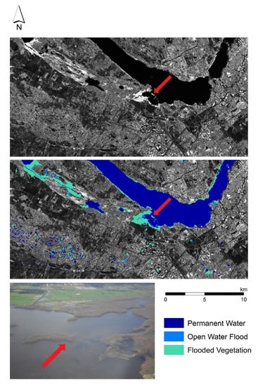
This study adds to a growing body of literature on the use of compact polarimetry for surface-water and wetland mapping. It presents a full set of CP parameters that produce the best open-water and flooded-vegetation mapping results, using EGSs’ machine learning and region growing methods for inundation mapping, which can also be applied to dense time-series for wetland identification and monitoring. It identifies CP parameters that show promise for surface-water mapping, regardless of the method used, and justifies them on statistical and physical bases, using a large number of scenes in three separate regions of Canada (Figure 6). It also supports and confirms the choice of parameters for flooded-vegetation mapping determined in other regions of Canada. We expect results to be transferrable to other parts of the world with similar vegetation; the results are also largely applicable to regions that are different, due to the universality of radar’s physical interactions with water.
5. Conclusions
The Emergency Geomatics Services has spent considerable effort developing open-water and flooded-vegetation mapping methods for near-real-time flood mapping that may also be useful to consistently and efficiently monitor wetland dynamics. Simulated RADARSAT Constellation Mission compact polarimetry has been shown to generate flood maps, including for open-water and flooded vegetation, that are consistent with current maps produced by EGS from RADARSAT-2. Using a stepwise classification procedure that entered CP parameters in order, based on a multi-criterion ranking that included variable importance, separability, and correlation, to remove redundant features, the top four parameters (mdelta/mchiVolume, RR, Sei, and RV) produced open-water maps consistent with baseline RADARSAT-2 maps when evaluated using omission, commission, and overall agreement. Separability analysis identified four promising parameters (RH, RR, SEi, and SV0) for regions growing flooded vegetation, based on intensity thresholds. An examination of intensity beneath known flooded-vegetation targets revealed a dependence on incidence angle, with two separate groups occurring at greater than and less than 30 degrees. By examining intensity values at each incidence angle range and through trial and error, thresholds were determined and applied to regions growing flooded vegetation, for each parameter and incidence angle. An assessment of flooded-vegetation maps showed that the most separable parameter (RH) had the lowest omission evaluated against delineated flooded-vegetation polygons, while differences were smaller between the four top parameters for commission evaluated on upland slopes, where flooding cannot occur. The 16 m Medium Resolution beam mode with a noise floor of −25 dB will likely be the requested beam mode for flood-response operations, providing the best combination of pixel resolution, noise floor, processing time, and swath width compared to the 5 m High Resolution and 30 m Medium Resolution beam modes. The final set of CP parameters required to run the full operational flood-mapping procedure includes both native parameters RH and RV, in addition to three derived parameters, mdelta/mchiVolume, RR and SEi. While further development would be required to add CP parameter generation to current flood tools, there are other projects currently underway at the CCMEO, with similar objectives. Toolboxes are being developed to create value-added products from RCM data, including deriving CP parameters such as the ones highlighted above. While these products would not be created in near real time, the underlying processes could potentially aid in accelerating the EGS’s tool development. Regardless, work is still needed to modify existing tools to ingest and process real RCM data’s file formats and directory structure. Additional testing will also be necessary upon reception of real RCM data, to validate the results obtained here.
Author Contributions
I.O. developed software, conceptualized the study and assembled and edited the final paper. T.R. conducted the analyses and wrote the initial draft. All authors have read and agreed to the published version of the manuscript.
Funding
Funding was provided by the Canadian Space Agency, under the RADARSAT Constellation Mission’s Data Utilization and Application Plan.
Acknowledgments
The authors would like to thank Brian Brisco, François Charbonneau, Torsten Geldzetser, Brad Lehrbass, and Joost van der Sanden for their input, review, and comments during the preparation of this article.
Conflicts of Interest
The authors declare no conflict of interest.
References
- Maltby, E.; Acreman, M.C. Ecosystem services of wetlands: Pathfinder for a new paradigm. Hydrol. Sci. J. 2011, 56, 1341–1359. [Google Scholar] [CrossRef]
- Keddy, P.A. Wetland Ecology: Principles and Conservation, 2nd ed.; Cambridge University Press: New York, NY, USA, 2010; ISBN 978-0521519403. [Google Scholar]
- Olthof, I. Mapping seasonal inundation frequency (1985–2016) along the St-John River, New Brunswick, Canada using the Landsat archive. Remote Sens. 2017, 9, 143. [Google Scholar] [CrossRef]
- Olthof, I.; Tolszczuk-Leclerc, S. Comparing landsat and RADARSAT for current and historical dynamic flood mapping. Remote Sens. 2018, 10, 780. [Google Scholar] [CrossRef] [Green Version]
- Brisco, B.; Short, N.; Van der Sanden, J.; Landry, R.; Raymond, D. A semi-automated tool for surface water mapping with RADARSAT-1. Can. J. Remote Sens. 2009, 35, 336–344. [Google Scholar] [CrossRef]
- Catry, T.; Li, Z.; Roux, E.; Herbreteau, V.; Gurgel, H.; Mangeas, M.; Seyler, F.; Dessay, N. Wetlands and Malaria in the Amazon: Guidelines for the Use of Synthetic Aperture Radar Remote-Sensing. Int. J. Environ. Res. Public Health 2018, 15, 468. [Google Scholar] [CrossRef] [Green Version]
- Kasischke, E.S.; Melack, J.M.; Craig Dobson, M. The use of imaging radars for ecological applications—A review. Remote Sens. Environ. 1997, 59, 141–156. [Google Scholar] [CrossRef]
- Lee, J.S.; Pottier, E. Polarimetric Radar Imaging: From Basics to Applications; CRC Press: Boca Raton, FL, USA, 2009. [Google Scholar] [CrossRef]
- Simpson, R.A.; Harmon, J.K.; Zisk, S.H.; Thompson, T.W.; Muhleman, D.O. Radar determination of Mars surface properties. In Mars; Kieffer, H.H., Jakosky, B.M., Snyder, C.W., Matthews, M.S., Eds.; University of Arizona Press: Tucson, AZ, USA, 1992; pp. 686–729. [Google Scholar]
- Baghdadi, N.; Bernier, M.; Gauthier, R.; Neeson, I. Evaluation of C-band SAR data for wetlands mapping. Int. J. Remote Sens. 2001, 22, 71–88. [Google Scholar] [CrossRef]
- Charbonneau, F.J.; Brisco, B.; Raney, R.K.; McNairn, H.; Liu, C.; Vachon, P.W.; Shang, J.; DeAbreu, R.; Champagne, C.; Merzouki, A.; et al. Compact polarimetry overview and applications assessment. Can. J. Remote Sens. 2010, 36 (Suppl. 2), S298–S315. [Google Scholar] [CrossRef]
- Bolanos, S.; Stiff, D.; Brisco, B.; Pietroniro, A. Operational surface water detection and monitoring using RADARSAT-2. Remote Sens. 2016, 8, 285. [Google Scholar] [CrossRef] [Green Version]
- Van der Sanden, J.J.; Geldsetzer, T. Compact polarimetry in support of lake ice breakup monitoring: Anticipating the RADARSAT Constellation Mission. Can. J. Remote Sens. 2015, 41, 440–457. [Google Scholar] [CrossRef]
- White, L.; Brisco, B.; Pregitzer, M.; Tedford, B.; Boychuk, L. RADARSAT-2 beam mode selection for surface water and flooded vegetation mapping. Can. J. Remote Sens. 2014, 40, 135–151. [Google Scholar] [CrossRef]
- Bourgeau-Chavez, L.L.; Kasischke, E.S.; Brunzell, S.M.; Mudd, J.P.; Smith, K.B.; Frick, A.L. Analysis of space-borne SAR data for wetland mapping in Virginia riparian ecosystems. Int. J. Remote Sens. 2001, 22, 3665–3687. [Google Scholar] [CrossRef]
- Hess, L.L.; Melack, J.M.; Filoso, S.; Wang, Y. Delineation of inundated area and vegetation along the Amazon floodplain with the SIR-C synthetic aperture radar. IEEE Trans. Geosci. Remote. Sens. 1995, 33, 896–904. [Google Scholar] [CrossRef] [Green Version]
- Raney, R.K. Hybrid-Polarity SAR Architecture. In Proceedings of the 2006 IEEE International Symposium on Geoscience and Remote Sensing, Denver, CO, USA, 31 July–4 August 2006; pp. 3846–3848. [Google Scholar] [CrossRef] [Green Version]
- Olthof, I.; Tolszczuk-Leclerc, S.; Lehrbass, B.; Shelat, Y.; Neufeld, V.; Decker, V. New flood mapping methods implemented during the 2017 spring flood activation in southern Quebec. Geomat. Can. 2018, 38, 16. [Google Scholar] [CrossRef]
- Canadian Wetland Inventory (CWI). Canadian Space Agency, Ducks Unlimited Canada, Environment Canada and North American Wetlands Conservation Council (Canada). 2020. Available online: https://maps.ducks.ca/cwi/ (accessed on 30 April 2020).
- R Core Team. R: A Language and Environment for Statistical Computing; R Foundation for Statistical Computing: Vienna, Austria, 2018; Available online: https://www.R-project.org/ (accessed on 30 April 2020).
- Olthof, I.; Tolszczuk-Leclerc, S.; Lerhbass, B.; Shelat, Y.; Neufeld, V.; Decker, V. Flood mapping from multi-sensor Earth Observation data for near real-time infrastructure impact assessment: Lessons learned from the 2017 spring flood in eastern Canada. In Advances in Remote Sensing for Infrastructure Monitoring; Singhroy, V., Ed.; Springer: New York, NY, USA, in press.
- Canadian Space Agency (CSA). Technical Characteristics. Available online: https://www.asc-csa.gc.ca/eng/satellites/radarsat/technical-features/characteristics.asp (accessed on 14 May 2019).
- Kuhn, M.; Quinlan, R. C50: C5.0 Decision Trees and Rule-Based Models. R Package Version 0.1.2. 2018. Available online: https://CRAN.R-project.org/package=C50 (accessed on 30 April 2020).
- Quinlan, R. C4.5: Programs for Machine Learning; Morgan Kaufmann Publishers: San Mateo, CA, USA, 1993. [Google Scholar]
- Pekel, J.-F.; Cottam, A.; Gorelick, N.; Belward, A.S. High-resolution mapping of global surface water and its long-term changes. Nature 2016, 540, 418–436. [Google Scholar] [CrossRef]
- Latifovic, R.; Pouliot, D.; Olthof, I. Circa 2010 land cover of Canada: Local optimization of methodology and product development. Remote Sens. 2017, 9, 1098. [Google Scholar] [CrossRef] [Green Version]
- Massey, F.J. The Kolmogorov-Smirnov test for goodness of fit. J. Am. Stat. Assoc. 1951, 46, 68–78. [Google Scholar] [CrossRef]
- Brisco, B.; Shelat, Y.; Murnaghan, K.; Montgomery, J.; Fuss, C.; Olthof, I.; Hopkinson, C.; Deschamps, A.; Poncos, V. Evaluation of C-band SAR for identification of flooded vegetation in emergency response products. Can. J. Remote Sens. 2019, 45, 73–87. [Google Scholar] [CrossRef]
- Mohammadimanesh, F.; Salehi, B.; Mahdianpari, M.; Brisco, B.; Gill, E. Full and simulated compact polarimetry SAR responses to canadian wetlands: Separability analysis and classification. Remote Sens. 2019, 11, 516. [Google Scholar] [CrossRef] [Green Version]
- Environment and Climate Change Canada (ECCC). Historical Hydrometric Data. Available online: https://wateroffice.ec.gc.ca/mainmenu/historical_data_index_e.html (accessed on 5 August 2019).
- Natural Resources Canada (NRCan). National Hydrographic Network. Available online: https://www.nrcan.gc.ca/science-and-data/science-and-research/earth-sciences/geography/topographic-information/geobase-surface-water-program-geeau/national-hydrographic-network/21361 (accessed on 25 April 2019).
- Congalton, R.G. A review of assessing the accuracy of classifications of remotely sensed data. Remote Sens. Environ. 1991, 37, 35–46. [Google Scholar] [CrossRef]
- Raney, R.K.; Cahill, J.T.S.; Patterson, G.W.; Bussey, D.B.J. The m-chi decomposition of hybrid dual-polarimetric radar data with application to lunar craters. J. Geophys. Res. 2012, 117, E00H21. [Google Scholar] [CrossRef]
- Raney, R.K. Hybrid dual-polarization synthetic aperture radar. Remote Sens. 2019, 11, 1521. [Google Scholar] [CrossRef] [Green Version]
- Marechal, C.; Pottier, E.; Hubert-Moy, L.; Rapinel, S. One year wetland survey investigations from quad-pol RADARSAT-2 time-series SAR images. Can. J. Remote Sens. 2012, 38, 240–252. [Google Scholar] [CrossRef]
- Morio, J.; Réfrégier, P.; Goudail, F.; Dubois-Fernandez, P.; Dupuis, X. Application of information theory measures to polarimetric and interferometric SAR images. In Proceedings of the 5th International Conference on Physics in Signal Image Processing, Mulhouse, France, 31 January–2 February 2007. [Google Scholar]
- Nobre, A.D.; Cuartas, L.A.; Hodnett, M.; Renno, C.D.; Rodrigues, G.; Silveira, A.; Waterloo, M.; Saleska, S. Height above the nearest drainage—A hydrologically relevant new terrain model. J. Hydrol. 2011, 404, 13–29. [Google Scholar] [CrossRef] [Green Version]
- Hess, L.L.; Melack, J.M.; Simonett, D.S. Radar detection of flood beneath the forest canopy: A review. Int. J. Remote Sens. 1990, 11, 1313–1325. [Google Scholar] [CrossRef]
Figure 1.
Coverage of sample scenes from the three flood-prone study regions in Eastern Canada.

Figure 2.
Overview of Compact Polarimetric feature selection for open-water and flooded-vegetation mapping.
Figure 2.
Overview of Compact Polarimetric feature selection for open-water and flooded-vegetation mapping.

Figure 3.
Processing time in relation to number of input parameters and pixel resolution.

Figure 4.
Mean flooded-vegetation polygon values versus mean scene incidence angle and chosen threshold values (horizontal dashed lines) for the top four CP parameters, showing highest separability between flooded vegetation and other land-cover classes.
Figure 4.
Mean flooded-vegetation polygon values versus mean scene incidence angle and chosen threshold values (horizontal dashed lines) for the top four CP parameters, showing highest separability between flooded vegetation and other land-cover classes.

Figure 5.
Simulated 16 m RADARSAT Constellation Mission (RCM) Right-Horizontal (RH) channel (top) from RS2 imagery acquired west of Ottawa, on 30 April 2017, showing bright areas characteristic of double-bounce interactions with flooded vegetation. The derived open-water and flooded-vegetation map (middle) and National Aerial Surveillance Program (NASP) oblique image acquired 15 May 2017, confirming vegetation flooding. The red arrow indicates the look direction.

Figure 6.
Emergency Geomatics Service (EGS) flood maps generated from R2 imagery (left column), with corresponding products generated from 16 m simulated RCM imagery (right column), over portions of the three study areas, using the best parameters determined from this study.
Figure 6.
Emergency Geomatics Service (EGS) flood maps generated from R2 imagery (left column), with corresponding products generated from 16 m simulated RCM imagery (right column), over portions of the three study areas, using the best parameters determined from this study.


Table 1.
RADARSAT-2 sample scene information.
| Region | Acquisition Date | Acquisition Start Time | Beam Mode | Pixel Resolution (m) [Rng × Az] | Average Incidence Angle (°) | Swath Width (km) [Rng × Az] | Flooded Vegetation Present |
|---|---|---|---|---|---|---|---|
| Ottawa | 02 April 2017 | 11:26:02 | Fine Quad Wide—FQ1W | 4.73 × 4.83 | 19.40 | 50 × 25 | No |
| Ottawa | 26 April 2017 | 11:26:01 | Fine Quad Wide—FQ1W | 4.73 × 4.83 | 19.41 | 50 × 25 | Yes |
| Ottawa | 30 April 2017 | 11:09:23 | Fine Quad Wide—FQ20W | 4.73 × 5.07 | 39.99 | 50 × 25 | Yes |
| Ottawa | 20 May 2017 | 11:26:00 | Fine Quad Wide—FQ1W | 4.73 × 4.83 | 19.40 | 50 × 25 | Yes |
| Ottawa | 24 May 2017 | 11:09:22 | Fine Quad Wide—FQ20W | 4.73 × 5.07 | 39.99 | 50 × 25 | No |
| Richelieu | 11 April 2011 | 10:57:34 | Fine Quad—FQ22 | 4.73 × 5.49 | 41.79 | 25 × 25 | Yes |
| Richelieu | 11 April 2011 | 10:57:37 | Fine Quad—FQ22 | 4.73 × 5.49 | 41.80 | 25 × 25 | Yes |
| Richelieu | 18April 2011 | 10:53:24 | Fine Quad—FQ27 | 4.73 × 4.86 | 45.90 | 25 × 25 | Yes |
| Richelieu | 18 April 2011 | 10:53:28 | Fine Quad—FQ27 | 4.73 × 4.86 | 45.90 | 25 × 25 | Yes |
| Richelieu | 05 May 2011 | 10:57:14 | Standard Quad—SQ21 | 11.83 × 5.13 | 40.92 | 25 × 25 | Yes |
| Richelieu | 05 May 2011 | 10:57:17 | Standard Quad—SQ21 | 11.83 × 5.13 | 40.92 | 25 × 25 | Yes |
| Richelieu | 08 May 2011 | 22:30:30 | Standard Quad—SQ2 | 7.98 × 4.87 | 20.85 | 25 × 25 | Yes |
| Richelieu | 08 May 2011 | 22:30:33 | Standard Quad—SQ2 | 7.98 × 4.87 | 20.85 | 25 × 25 | Yes |
| Richelieu | 22 May 2011 | 11:01:32 | Fine Quad—FQ17 | 4.73 × 5.47 | 37.23 | 25 × 25 | Yes |
| Richelieu | 22 May 2011 | 11:01:44 | Fine Quad—FQ17 | 4.73 × 5.47 | 37.23 | 25 × 25 | Yes |
| Saint John | 04 July 2008 | 10:44:03 | Fine Quad—FQ8 | 4.73 × 4.78 | 27.85 | 25 × 25 | Yes |
| Saint John | 19 May 2009 | 10:40:13 | Fine Quad—FQ11 | 4.73 × 5.59 | 31.14 | 25 × 25 | Yes |
| Saint John | 27 April 2010 | 10:36:15 | Fine Quad—FQ16 | 4.73 × 5.16 | 36.27 | 25 × 25 | Yes |
| Saint John | 21 May 2010 | 10:36:14 | Fine Quad—FQ16 | 4.73 × 5.16 | 36.27 | 25 × 25 | No |
Table 2.
Assumed specifications of selected RADARSAT Constellation Mission beam modes.
| Beam Mode | Resolution (m) | Noise Floor/Nominal NESZ (dB) | Swath Width (km) | Looks (Rng × Az) |
|---|---|---|---|---|
| 5 m High Resolution | 5 | −19 | 30 | 1 × 1 |
| 16 m Medium Resolution | 16 | −25 | 30 | 1 × 4 |
| 30 m Medium Resolution | 30 | −24 | 125 | 2 × 2 |
Table 3.
Simulated compact polarimetric parameters, corresponding equations, and identifying variable names used in this study.
Table 3.
Simulated compact polarimetric parameters, corresponding equations, and identifying variable names used in this study.
| Compact Polarimetric Parameter | Variable Name(s) | Equation |
|---|---|---|
| Alpha S angle | alphaS | |
| Circular polarization ratio | circ | |
| Conformity coefficient | conformity | |
| Relative phase between RV and RH | delta | |
| Degree of polarization | m | |
| m-chi decomposition ▪ Even-bounce ▪ Volume ▪ Odd-bounce | mchiEven mchiVolume mchiOdd | |
| m-delta decomposition ▪ Even-bounce ▪ Volume ▪ Odd-bounce | mdeltaEven mdeltaVolume mdeltaOdd | |
| Correlation coefficient of RV and RH | rho/rhoAdjust | |
| Intensity channels ▪ 4 channels | RH RV RR RL | |
| Shannon entropy ▪ Intensity ▪ Polarimetric | SEi SEp | |
| Stokes vector ▪ 4 elements | SV0 SV1 SV2 SV3 |
Table 4.
Total attribute usage points for each compact polarimetric (CP) parameter, across regions and beam modes.
Table 4.
Total attribute usage points for each compact polarimetric (CP) parameter, across regions and beam modes.
| Ottawa | Richelieu | Saint John | Total | |||||||
|---|---|---|---|---|---|---|---|---|---|---|
| Parameter | 5 m | 16 m | 30 m | 5 m | 16 m | 30 m | 5 m | 16 m | 30 m | |
| mdeltaVolume | 22 | 22 | 22 | 22 | 22 | 22 | 20 | 19 | 20 | 191 |
| RH | 18 | 19 | 20 | 21 | 21 | 21 | 22 | 22 | 21 | 185 |
| RR | 21 | 21 | 21 | 18 | 19 | 18 | 18 | 21 | 22 | 179 |
| SEi | 20 | 20 | 18 | 19 | 18 | 19 | 17 | 18 | 17 | 166 |
| RL | 17 | 14 | 15 | 20 | 20 | 20 | 21 | 20 | 19 | 166 |
| SEp | 19 | 18 | 19 | 15 | 16 | 17 | 15 | 13 | 15 | 147 |
| SV0 | 16 | 17 | 16 | 17 | 12 | 14 | 19 | 16 | 16 | 143 |
| RV | 12 | 15 | 11 | 13 | 15 | 13 | 16 | 17 | 18 | 130 |
| SV2 | 10 | 11 | 10 | 14 | 14 | 15 | 14 | 14 | 13 | 115 |
| SV1 | 11 | 9 | 9 | 16 | 17 | 16 | 11 | 12 | 10 | 111 |
| conformity | 14 | 16 | 17 | 6 | 4 | 8 | 12 | 15 | 4 | 96 |
| m | 13 | 12 | 12 | 12 | 13 | 12 | 7 | 5 | 9 | 95 |
| rhoAdjust | 15 | 10 | 14 | 10 | 9 | 10 | 9 | 4 | 6 | 87 |
| circ | 9 | 8 | 13 | 2 | 5 | 6 | 13 | 10 | 14 | 80 |
| SV3 | 7 | 13 | 8 | 11 | 8 | 9 | 6 | 2 | 5 | 69 |
| mchiEven | 8 | 7 | 7 | 8 | 11 | 11 | 2 | 8 | 3 | 65 |
| mdeltaEven | 4 | 5 | 4 | 7 | 7 | 7 | 8 | 7 | 7 | 56 |
| mdeltaOdd | 5 | 3 | 3 | 4 | 3 | 3 | 10 | 11 | 12 | 54 |
| delta | 3 | 6 | 6 | 5 | 6 | 5 | 3 | 9 | 8 | 51 |
| mchiOdd | 6 | 2 | 5 | 3 | 2 | 2 | 4 | 6 | 11 | 41 |
| alphaS | 2 | 4 | 2 | 9 | 10 | 4 | 5 | 3 | 2 | 41 |
| mchiVolume | 1 | 1 | 1 | 1 | 1 | 1 | 1 | 1 | 1 | 9 |
Table 5.
Total open-water separability points for each CP parameter, across regions and beam modes.
| Ottawa | Richelieu | Saint John | ||||||||
|---|---|---|---|---|---|---|---|---|---|---|
| Parameter | 5 m | 16 m | 30 m | 5 m | 16 m | 30 m | 5 m | 16 m | 30 m | Total |
| mchiVolume | 25 | 25 | 25 | 33 | 33 | 33 | 14 | 14 | 13 | 215 |
| mdeltaVolume | 25 | 25 | 25 | 33 | 33 | 33 | 14 | 14 | 13 | 215 |
| RR | 24 | 24 | 24 | 33 | 33 | 33 | 13 | 14 | 13 | 211 |
| RH | 12 | 12 | 12 | 26 | 26 | 26 | 14 | 14 | 14 | 156 |
| SEi | 12 | 12 | 12 | 26 | 26 | 26 | 14 | 14 | 14 | 156 |
| SV0 | 12 | 12 | 12 | 26 | 26 | 26 | 14 | 14 | 14 | 156 |
| RL | 11 | 11 | 11 | 21 | 22 | 23 | 15 | 15 | 13 | 142 |
| RV | 9 | 10 | 9 | 22 | 23 | 23 | 13 | 15 | 13 | 137 |
| mchiEven | 12 | 14 | 14 | 19 | 22 | 23 | 1 | 1 | 1 | 107 |
| mdeltaEven | 9 | 11 | 11 | 15 | 20 | 19 | 0 | 0 | 0 | 85 |
| mchiOdd | 4 | 6 | 5 | 10 | 12 | 12 | 11 | 11 | 10 | 81 |
| mdeltaOdd | 0 | 1 | 1 | 5 | 9 | 9 | 10 | 10 | 10 | 55 |
| SV1 | 3 | 3 | 3 | 12 | 12 | 12 | 1 | 1 | 1 | 48 |
| circ | 2 | 6 | 6 | 6 | 11 | 10 | 0 | 0 | 0 | 41 |
| conformity | 2 | 6 | 6 | 6 | 11 | 10 | 0 | 0 | 0 | 41 |
| SV3 | 1 | 1 | 1 | 4 | 4 | 4 | 8 | 9 | 8 | 40 |
| alphaS | 1 | 3 | 3 | 5 | 8 | 8 | 0 | 0 | 0 | 28 |
| SEp | 2 | 6 | 4 | 0 | 2 | 1 | 0 | 0 | 0 | 15 |
| rhoAdjust | 1 | 2 | 3 | 0 | 3 | 2 | 0 | 0 | 0 | 11 |
| delta | 0 | 0 | 1 | 2 | 3 | 4 | 0 | 0 | 0 | 10 |
| m | 1 | 2 | 3 | 0 | 2 | 2 | 0 | 0 | 0 | 10 |
| SV2 | 1 | 1 | 1 | 1 | 2 | 3 | 0 | 0 | 0 | 9 |
Table 6.
Total correlation points for each CP parameter, across regions and beam modes.
| Ottawa (n = 5) | Richelieu (n = 10) | Saint John (n = 4) | ||||||||
|---|---|---|---|---|---|---|---|---|---|---|
| Parameter | 5 m | 16 m | 30 m | 5 m | 16 m | 30 m | 5 m | 16 m | 30 m | Total |
| SV1 | 5 | 5 | 5 | 10 | 10 | 10 | 4 | 4 | 4 | 57 |
| SV2 | 5 | 5 | 5 | 10 | 10 | 10 | 4 | 4 | 4 | 57 |
| delta | 5 | 5 | 5 | 10 | 9 | 10 | 4 | 4 | 4 | 56 |
| m | 3 | 5 | 5 | 9 | 9 | 9 | 3 | 3 | 3 | 49 |
| mdeltaEven | 4 | 4 | 4 | 6 | 8 | 8 | 4 | 4 | 4 | 46 |
| SEp | 2 | 2 | 2 | 7 | 7 | 7 | 4 | 4 | 4 | 39 |
| RV | 2 | 4 | 3 | 6 | 4 | 6 | 1 | 1 | 1 | 28 |
| mdeltaVolume | 4 | 3 | 3 | 5 | 1 | 1 | 2 | 2 | 2 | 23 |
| SV3 | 2 | 2 | 2 | 2 | 4 | 4 | 0 | 0 | 0 | 16 |
| SEi | 2 | 3 | 4 | 1 | 3 | 2 | 0 | 0 | 0 | 15 |
| alphaS | 2 | 1 | 1 | 1 | 2 | 2 | 2 | 2 | 2 | 15 |
| mdeltaOdd | 3 | 2 | 3 | 0 | 0 | 0 | 1 | 1 | 1 | 11 |
| mchiOdd | 0 | 0 | 0 | 1 | 3 | 2 | 0 | 0 | 0 | 6 |
| rhoAdjust | 1 | 0 | 0 | 0 | 0 | 0 | 1 | 1 | 1 | 4 |
| mchiVolume | 0 | 0 | 0 | 0 | 0 | 0 | 1 | 1 | 1 | 3 |
| mchiEven | 0 | 0 | 0 | 0 | 1 | 1 | 0 | 0 | 0 | 2 |
| RL | 0 | 0 | 0 | 0 | 1 | 1 | 0 | 0 | 0 | 2 |
| circ | 0 | 0 | 0 | 0 | 0 | 0 | 0 | 0 | 0 | 0 |
| conformity | 0 | 0 | 0 | 0 | 0 | 0 | 0 | 0 | 0 | 0 |
| RH | 0 | 0 | 0 | 0 | 0 | 0 | 0 | 0 | 0 | 0 |
| RR | 0 | 0 | 0 | 0 | 0 | 0 | 0 | 0 | 0 | 0 |
| SV0 | 0 | 0 | 0 | 0 | 0 | 0 | 0 | 0 | 0 | 0 |
Table 7.
Normalized final point ranking of all compact polarimetric parameters.
| Parameter | Attribute Usage | Separability | Correlation | Normalized Points |
|---|---|---|---|---|
| mdeltaVolume | 1.00 | 1.00 | 0.40 | 2.40 |
| RR | 0.94 | 0.98 | 0.00 | 1.92 |
| SEi | 0.87 | 0.73 | 0.26 | 1.85 |
| RV | 0.68 | 0.64 | 0.49 | 1.81 |
| SV1 | 0.58 | 0.22 | 1.00 | 1.80 |
| RH | 0.97 | 0.73 | 0.00 | 1.69 |
| SV2 | 0.60 | 0.04 | 1.00 | 1.64 |
| RL | 0.87 | 0.66 | 0.04 | 1.56 |
| SEp | 0.77 | 0.07 | 0.68 | 1.52 |
| mdeltaEven | 0.29 | 0.40 | 0.81 | 1.50 |
| SV0 | 0.75 | 0.73 | 0.00 | 1.47 |
| m | 0.50 | 0.05 | 0.86 | 1.40 |
| delta | 0.27 | 0.05 | 0.98 | 1.30 |
| mchiVolume | 0.05 | 1.00 | 0.05 | 1.10 |
| mchiEven | 0.34 | 0.50 | 0.04 | 0.87 |
| SV3 | 0.36 | 0.19 | 0.28 | 0.83 |
| mdeltaOdd | 0.28 | 0.26 | 0.19 | 0.73 |
| mchiOdd | 0.21 | 0.38 | 0.11 | 0.70 |
| conformity | 0.50 | 0.19 | 0.00 | 0.69 |
| circ | 0.42 | 0.19 | 0.00 | 0.61 |
| alphaS | 0.21 | 0.13 | 0.26 | 0.61 |
| rhoAdjust | 0.46 | 0.05 | 0.07 | 0.58 |
Table 8.
Number of scenes showing lowest omission and commission and highest overall agreement of open-water classifications, based on number of input parameters across study regions and beam modes.
Table 8.
Number of scenes showing lowest omission and commission and highest overall agreement of open-water classifications, based on number of input parameters across study regions and beam modes.
| Lowest Omission | Lowest Commission | Highest Overall Agreement | ||||||||||||||
|---|---|---|---|---|---|---|---|---|---|---|---|---|---|---|---|---|
| # Parameters → Beam Mode ↓ | 1 | 2 | 3 | 4 | 5 | 1 | 2 | 3 | 4 | 5 | 1 | 2 | 3 | 4 | 5 | |
| Ottawa | 5 m | 0 | 1 | 1 | 2 | 1 | 0 | 0 | 3 | 1 | 1 | 0 | 0 | 2 | 2 | 1 |
| 16 m | 1 | 1 | 3 | 0 | 0 | 0 | 1 | 0 | 3 | 1 | 0 | 0 | 1 | 2 | 2 | |
| 30 m | 1 | 2 | 1 | 1 | 0 | 1 | 1 | 0 | 2 | 1 | 0 | 0 | 1 | 1 | 3 | |
| % Scenes | 13.33 | 26.67 | 33.33 | 20.00 | 6.67 | 6.67 | 13.33 | 20.00 | 40.00 | 20.00 | 0.00 | 0.00 | 28.57 | 35.71 | 35.71 | |
| Richelieu | 5 m | 5 | 1 | 1 | 3 | 0 | 0 | 2 | 1 | 1 | 6 | 0 | 0 | 1 | 4 | 5 |
| 16 m | 6 | 2 | 2 | 0 | 0 | 1 | 2 | 0 | 2 | 5 | 1 | 1 | 3 | 3 | 2 | |
| 30 m | 5 | 3 | 0 | 1 | 1 | 1 | 2 | 0 | 2 | 5 | 2 | 1 | 0 | 3 | 4 | |
| % Scenes | 53.33 | 20.00 | 10.00 | 13.33 | 3.33 | 6.67 | 20.00 | 3.33 | 16.67 | 53.33 | 10.00 | 6.67 | 13.33 | 33.33 | 36.67 | |
| Saint John | 5 m | 3 | 0 | 0 | 1 | 0 | 0 | 0 | 1 | 0 | 3 | 0 | 0 | 0 | 3 | 1 |
| 16 m | 1 | 2 | 0 | 1 | 0 | 0 | 0 | 3 | 0 | 1 | 1 | 1 | 0 | 2 | 1 | |
| 30 m | 3 | 1 | 0 | 0 | 0 | 0 | 0 | 1 | 2 | 1 | 0 | 1 | 0 | 2 | 1 | |
| % Scenes | 58.33 | 25.00 | 0.00 | 16.67 | 0.00 | 0.00 | 0.00 | 41.67 | 16.67 | 41.67 | 7.69 | 15.38 | 0.00 | 53.85 | 23.08 | |
Table 9.
Average omission, commission, and overall agreement of open-water classifications, based on number of input parameters across regions, compared to baseline 22 CP parameter classifications. The best results of the one-to-five input parameter trials are highlighted in green, and cases where the 22 CP parameter trial was best are also highlighted in blue.
| Number of Input Parameters | |||||||
|---|---|---|---|---|---|---|---|
| 1 | 2 | 3 | 4 | 5 | 22 | ||
| Omission | Ottawa | 12.55 | 12.29 | 11.07 | 10.69 | 10.42 | 10.26 |
| Richelieu | 4.03 | 6.30 | 4.76 | 4.66 | 4.61 | 5.35 | |
| Saint John | 17.67 | 20.45 | 26.47 | 20.03 | 20.74 | 20.70 | |
| Commission | Ottawa | 11.21 | 11.19 | 9.53 | 9.30 | 9.39 | 9.37 |
| Richelieu | 5.19 | 4.14 | 4.06 | 3.98 | 3.93 | 3.92 | |
| Saint John | 21.49 | 20.23 | 17.04 | 17.74 | 17.62 | 17.49 | |
| Overall Agreement | Ottawa | 98.90 | 98.92 | 99.07 | 99.09 | 99.10 | 99.11 |
| Richelieu | 98.78 | 98.76 | 98.85 | 98.86 | 98.90 | 98.89 | |
| Saint John | 99.57 | 99.57 | 99.57 | 99.60 | 99.60 | 99.61 | |
Table 10.
Total flooded vegetation separability points for each CP parameter, across regions and beam modes.
Table 10.
Total flooded vegetation separability points for each CP parameter, across regions and beam modes.
| Ottawa | Richelieu | Saint John | ||||||||
|---|---|---|---|---|---|---|---|---|---|---|
| Parameter | 5 m | 16 m | 30 m | 5 m | 16 m | 30 m | 5 m | 16 m | 30 m | Total |
| RH | 20 | 20 | 20 | 17 | 17 | 18 | 20 | 21 | 20 | 173 |
| RR | 22 | 22 | 22 | 19 | 20 | 20 | 10 | 11 | 11 | 157 |
| SEi | 17 | 18 | 18 | 15 | 15 | 16 | 19 | 19 | 19 | 156 |
| SV0 | 17 | 18 | 18 | 15 | 15 | 16 | 19 | 19 | 19 | 156 |
| mchiEven | 15 | 16 | 16 | 18 | 19 | 19 | 5 | 5 | 5 | 118 |
| mdeltaEven | 13 | 13 | 13 | 17 | 17 | 18 | 3 | 4 | 4 | 102 |
| SV1 | 15 | 15 | 15 | 14 | 14 | 15 | 1 | 1 | 1 | 91 |
| mchiVolume | 10 | 12 | 12 | 8 | 10 | 11 | 8 | 8 | 7 | 86 |
| mdeltaVolume | 10 | 12 | 12 | 8 | 10 | 11 | 8 | 8 | 7 | 86 |
| RL | 8 | 9 | 10 | 5 | 5 | 6 | 11 | 11 | 10 | 75 |
| alphaS | 5 | 6 | 6 | 9 | 10 | 11 | 6 | 6 | 6 | 65 |
| circ | 2 | 2 | 2 | 7 | 9 | 10 | 9 | 9 | 9 | 59 |
| conformity | 2 | 2 | 2 | 7 | 9 | 10 | 9 | 9 | 9 | 59 |
| RV | 4 | 4 | 4 | 5 | 5 | 6 | 10 | 11 | 9 | 58 |
| SV3 | 1 | 1 | 1 | 7 | 7 | 8 | 10 | 10 | 10 | 55 |
| delta | 1 | 1 | 2 | 7 | 7 | 8 | 0 | 0 | 0 | 26 |
| SV2 | 4 | 4 | 4 | 2 | 2 | 2 | 0 | 0 | 0 | 18 |
| SEp | 2 | 2 | 2 | 0 | 2 | 1 | 2 | 2 | 2 | 15 |
| m | 1 | 0 | 1 | 0 | 0 | 1 | 10 | 0 | 0 | 13 |
| mchiOdd | 0 | 0 | 0 | 1 | 1 | 2 | 2 | 2 | 1 | 9 |
| mdeltaOdd | 0 | 0 | 0 | 0 | 0 | 1 | 1 | 1 | 1 | 4 |
| rhoAdjust | 1 | 0 | 1 | 0 | 0 | 1 | 0 | 0 | 0 | 3 |
Table 11.
Flooded-vegetation omission and commission for all scenes for top four CP parameters found most separable between flooded vegetation and other land-cover classes.
Table 11.
Flooded-vegetation omission and commission for all scenes for top four CP parameters found most separable between flooded vegetation and other land-cover classes.
| Omission | Commission | ||||||||
|---|---|---|---|---|---|---|---|---|---|
| Scene Dates | RH | RR | SEi | SV0 | RH | RR | SEi | SV0 | |
| Ottawa | 26 April 2017—112601 | 25.64 | 67.39 | 27.00 | 32.24 | 2.02 | 1.02 | 3.07 | 2.43 |
| 30 April 2017—110923 | 17.79 | 18.44 | 32.41 | 33.40 | 3.25 | 2.36 | 2.13 | 2.04 | |
| 20 May 2017—112600 | 68.49 | 100.00 | 72.25 | 98.57 | 0.77 | 0.51 | 1.04 | 0.81 | |
| Richelieu | 11 April 2011—105734 | 12.67 | 14.14 | 33.43 | 35.63 | 14.59 | 8.80 | 9.10 | 8.45 |
| 11 April 2011—105737 | 16.29 | 17.89 | 37.49 | 40.63 | 15.98 | 12.06 | 11.12 | 10.88 | |
| 18 April 2011—105324 | 17.83 | 16.73 | 39.53 | 42.31 | 5.44 | 4.75 | 3.53 | 3.56 | |
| 18 April 2011—105328 | 16.52 | 16.09 | 39.94 | 47.66 | 6.75 | 5.70 | 4.63 | 4.53 | |
| 05 May 2011—105714 | 9.84 | 11.90 | 26.44 | 28.04 | 16.48 | 12.47 | 13.10 | 12.79 | |
| 05 May 2011—105717 | 5.61 | 6.42 | 17.33 | 18.84 | 11.89 | 8.36 | 7.74 | 7.70 | |
| 08 May 2011—223030 | 10.85 | 60.18 | 12.80 | 20.64 | 4.17 | 3.63 | 5.48 | 4.31 | |
| 08 May 2011—223033 | 11.69 | 41.08 | 13.97 | 24.32 | 2.42 | 2.00 | 3.88 | 3.15 | |
| 22 May 2011—110132 | 6.30 | 9.63 | 19.18 | 21.09 | 16.49 | 13.10 | 13.72 | 13.55 | |
| 22 May 2011—110144 | 35.00 | 45.38 | 71.50 | 73.38 | 2.15 | 1.40 | 1.23 | 1.21 | |
| Saint John | 04 July 2008—104403 | 100.00 | 100.00 | 35.94 | 98.68 | 0.88 | 0.80 | 1.28 | 1.03 |
| 19 May 2009—104013 | 12.39 | 38.69 | 51.40 | 52.59 | 4.52 | 2.25 | 2.28 | 2.11 | |
| 27 April 2010—103615 | 16.72 | 52.24 | 85.82 | 86.05 | 0.31 | 0.23 | 0.16 | 0.16 | |
| Average | 23.98 | 38.51 | 38.53 | 47.13 | 6.76 | 4.96 | 5.22 | 4.92 | |
| # Lowest Cases | 13 | 2 | 1 | 0 | 0 | 7 | 3 | 7 | |
© 2020 by the authors. Licensee MDPI, Basel, Switzerland. This article is an open access article distributed under the terms and conditions of the Creative Commons Attribution (CC BY) license (http://creativecommons.org/licenses/by/4.0/).
Share and Cite
MDPI and ACS Style
Olthof, I.; Rainville, T. Evaluating Simulated RADARSAT Constellation Mission (RCM) Compact Polarimetry for Open-Water and Flooded-Vegetation Wetland Mapping. Remote Sens. 2020, 12, 1476. https://doi.org/10.3390/rs12091476
AMA Style
Olthof I, Rainville T. Evaluating Simulated RADARSAT Constellation Mission (RCM) Compact Polarimetry for Open-Water and Flooded-Vegetation Wetland Mapping. Remote Sensing. 2020; 12(9):1476. https://doi.org/10.3390/rs12091476
Chicago/Turabian StyleOlthof, Ian, and Thomas Rainville. 2020. "Evaluating Simulated RADARSAT Constellation Mission (RCM) Compact Polarimetry for Open-Water and Flooded-Vegetation Wetland Mapping" Remote Sensing 12, no. 9: 1476. https://doi.org/10.3390/rs12091476
Note that from the first issue of 2016, this journal uses article numbers instead of page numbers. See further details here.