Causal Analysis of Accuracy Obtained Using High-Resolution Global Forest Change Data to Identify Forest Loss in Small Forest Plots


1
Department of Forest Management, Forestry and Forest Products Research Institute, 1 Matsunosato, Tsukuba, Ibaraki 305-8687, Japan
2
Faculty of Human Sciences, Waseda University, 2-579-15 Mikajima, Tokorozawa, Saitama 359-1192, Japan
*
Author to whom correspondence should be addressed.
Remote Sens. 2020, 12(15), 2489; https://doi.org/10.3390/rs12152489
Submission received: 24 June 2020
/
Revised: 30 July 2020
/
Accepted: 1 August 2020
/
Published: 3 August 2020
(This article belongs to the Special Issue Monitoring of Forest Ecological Environment Based on Remote Sensing Technology)
Abstract
:Identifying areas of forest loss is a fundamental aspect of sustainable forest management. Global Forest Change (GFC) datasets developed by Hansen et al. (in Science 342:850–853, 2013) are publicly available, but the accuracy of these datasets for small forest plots has not been assessed. We used a forest-wide polygon-based approach to assess the accuracy of using GFC data to identify areas of forest loss in an area containing numerous small forest plots. We evaluated the accuracy of detection of individual forest-loss polygons in the GFC dataset in terms of a “recall ratio”, the ratio of the spatial overlap of a forest-loss polygon determined from the GFC dataset to the area of a corresponding reference forest-loss polygon, which we determined by visual interpretation of aerial photographs. We analyzed the structural relationships of recall ratio with area of forest loss, tree species, and slope of the forest terrain by using linear non-Gaussian acyclic modelling. We showed that only 11.1% of forest-loss polygons in the reference dataset were successfully identified in the GFC dataset. The inferred structure indicated that recall ratio had the strongest relationships with area of forest loss, forest tree species, and height of the forest canopy. Our results indicate the need for careful consideration of structural relationships when using GFC datasets to identify areas of forest loss in regions where there are small forest plots. Moreover, further studies are required to examine the structural relationships for accuracy of land-use classification in forested areas in various regions and with different forest characteristics.
1. Introduction
Because forest losses greatly affect the benefits derived from the preservation of ecosystems [1,2,3], understanding their spatial distribution is important for effective forest management. Many research projects have identified the ecological importance of the spatial patterns of forest and areas of forest degradation or loss [4,5]. For example, forest loss in riparian areas often results in deterioration of stream water quality [6,7,8]. However, appropriate application of a mosaic approach to early stage reforestation can improve biodiversity by providing habitats for specific species [9,10]. Understanding the regional distribution of areas of forest, forest loss, and forest degradation is also useful for taking stock of the current situation, predicting future conditions, and undertaking sustainable forest planning [11,12,13]. Thus, detecting forest losses is a fundamental requirement for sustainable forest management.
Monitoring forest disturbances is a major interest in the remote-sensing community and many researchers have produced forest disturbance maps based on time-series satellite imagery at regional or broader scales [14,15,16]. The global forest change (GFC) dataset provides annual public domain maps of global forest loss [17] that have allowed researchers without specialist expertise in processing of remote sensing data to analyze spatial and temporal forest loss. The dataset publicly provides worldwide forest cover and change of forest cover maps at 30-m resolution, derived mainly from Landsat archives dating back to 2000.
Although it was developed on a global scale, the GFC dataset has been used in various fields at regional or local scale, for example, for estimations of carbon flux [18,19], for government policy assessments [20,21], and for biodiversity conservation programs [22,23]. It is, therefore, important to understand its accuracy at regional and local scale, where inaccurate data might compromise its use for forest management [24]. Some researchers have attempted to verify the accuracy of regional forest loss maps based on the GFC dataset by using pixel-based sampling points to ground-truth larger-scale regional map areas [25,26]. However, forest loss generally affects landscape units with clear areal extents, so such assessments are inappropriate at the level of forest stand or forest management unit [27]. Linke et al. reported that the probabilities of detecting forest harvesting at regional scale were sufficiently high if a polygon-based approach was used. They showed that 85% of GFC-based forest-loss polygons in a temperate forest region of Canada overlapped with more than half of those of the provincial forest harvest inventory [28]. Although their results held promise for establishing the regional accuracy of the GFC dataset, their study area was well suited to satellite image classification in that each reference area was more than 1 ha and the regional topography was of relatively low relief. The results of assessments of the regional accuracy of the GFC dataset in less favorable regions might produce different results. For example, it might be difficult to detect smaller patches (<1 ha) of forest loss in areas of steep terrain. To date, we know of no assessments of the accuracy of the GFC dataset for regional analyses of small areas of forest loss in regions of rugged topography.
The objective of this study was to evaluate the accuracy of the GFC dataset for detection of forest loss in regions of rugged terrain where there are small privately owned forest plots. In such regions, small areas of forest loss may compromise high-precision land classification. We investigated the accuracy by comparing polygonal areas of forest loss defined by the GFC dataset with a reference dataset of polygons of forest-loss data that we interpreted from aerial photographs covering our entire study area. We then investigated the structural relationships of accuracy of the GFC data to area of forest loss, forest species, and local slope. Finally, we considered the effectiveness of the GFC dataset as a tool to detect forest loss in our study area.
2. Materials and Methods
2.1. Study Area
Our study area is in the Bungo-Ono municipality of Oita Prefecture, south-west Japan (centered on 32°58′N, 131°35′E; Figure 1a,b). Its total area is 60,314 ha and it includes 44,659 ha of forest. Apart from areas of urban development and cropland, almost all of the study area is mountainous, with a mean slope of 28.8° in forested areas. The region is dominated by plantations of Japanese cedar (Cryptomeria japonica), Japanese cypress (Chamaecyparis obtusa), and red pine (Pinus densiflora), and deciduous broad-leaved forest including sawtooth oak (Quercus acutissima) (Figure 1c). Within the study area, 84% of the forested area is privately owned and 69% of the private forest plots are of less than 1 ha in area. Forestry is a major industry in the region and timber supply in the region has been required to meet increasing demand in recent years. Because there have been no large-scale natural disasters in the region for at least a decade, human activities have been the main cause of forest loss. Most of the harvesting of timber in the study area during the recent decades has been by clear-cutting; there have been episodes of moderate forest thinning.
2.2. Data
2.2.1. Reference Data
We generated a reference map of areas of forest loss by using aerial photographs acquired in 2014 and 2016 (Figure 2a,b). In 2014, photos were taken of the northern part of the study area on 1 June and those of the southern part on 9 September. In 2016, photos were taken of the entire study area on 8 December. We generated three-dimensional point clouds from both vintages of aerial photographs by using the Structure from Motion approach in PhotoScan Professional software (Agisoft LLC, Saint-Petersburg, Russian Federation). Both point clouds were then converted to digital surface models (DSMs) and ortho-images were produced at 0.5-m resolution. Then, the 2016 DSM was subtracted from the 2014 DSM and locations where the difference exceeded 5 m were extracted to represent areas of forest loss between 2014 and 2016. The forest loss map for the entire study area was then visually checked for credibility. We used the 2014 ortho-images to visually identify four categories of forest species present at that time, Japanese cedar, cypress, red pine, broad-leaved trees, as well as non-forested areas. Given the high resolution of the aerial photographs and the careful interpretation of the aerial photographs, the uncertainty in the reference dataset was considered to be sufficiently small.
2.2.2. Global Forest Cover Change Datasets
We used the 10° lat × 10° long annual forest-loss map data (top left corner at 40°N, 130°E) from the GFC dataset ver. 1.6 [17] and used SAGA GIS v.2.3.2 open-source software to vectorize the data. To cover the period of our reference forest-loss map, we extracted polygons for forest losses from June 2014 to December 2016 and masked the data outside our study area (Figure 2c,d).
2.3. Accuracy Assessment
To assess the accuracy of the GFC dataset we compared the areal extent, local slope, and tree species of the forest-loss polygons obtained from the GFC dataset with those from our reference dataset. Because forests of the study area are too dense to generate digital terrain model (DTM) from aerial photographs, slope was calculated at 5-m resolution based on a 5-m DTM published by the Geospatial Information Authority of Japan. The raster ortho-image showing the initial (2014) tree species was resampled to 5-m resolution to reduce computation time and then masked with the forest-loss polygons derived from the 2016 GFC forest-loss or the reference dataset. Areas classified as non-forest were included in forest-loss polygons because the raster image that we used for land classification was resampled to a lower resolution; consequently, the edges of some of the polygons categorized as forest loss may actually represent non-forest areas (Figure 3).
To quantify the accuracy of the GFC dataset in our study area, we used a method developed by Linke et al. [28]. We overlaid the forest-loss polygons of the reference data and GFC data and calculated the areas of overlap. We defined the ratio of the area of overlap of each GFC polygon to the entire area of the corresponding reference polygon as the “recall ratio”, and the ratio of the area of overlap of each GFC polygon with the corresponding reference polygon to the entire area of the GFC polygon as the “precision ratio” (Figure 4). We considered reference polygons with high recall ratios to have been detected in the GFC dataset, and GFC polygons with high precision ratios to have detected the forest loss of the reference data.
To investigate the influence of polygon area on the accuracy of the GFC dataset, we estimated the distributions of recall and precision ratios for five ranges of reference and GFC polygon area (ha) determined on the basis of the number of GFC raster cells they enclosed: ≤36, >0.36–0.81, >0.81–1.44, >1.44–2.25, and >2.25 ha. For our calculation of precision ratios, we used GFC polygons showing forest loss only between the summers of 2014 and 2016, because those showing forest losses between the summers of 2016 and 2017 included losses outside the range of the reference data (i.e., from the summer of 2014 and winter of 2016).
Reference forest-loss polygons with recall ratios >50% were considered to have been successfully detected by from the GFC dataset. Likewise, GFC forest-loss polygons with precision ratios >50% were considered to have successfully detected the forest loss of the reference dataset. We also compared the proportions of the areas of these polygons for the five ranges of reference polygon area defined above.
We made all of the above calculations by using the Pandas v. 1.0.3 and Geopandas v. 0.7.0 modules of the Python v. 3.8.1 programing language. The confidence intervals of the accuracies were not required, because of the forest-wide assessment approach we used in this study.
2.4. Inferences on a Structural Relationship
For local forest management, overlooking the occurrence of forest loss should be avoided in order to reduce disaster risk. Determining whether factors such as the size of the areas of forest loss or the local slope directly influence the accuracy of forest loss determined from the GFC dataset (and if so, by how much) should further indicate the utility of the GFC data for this purpose. Since identifying where omission occurs is important in local forest management, relationships between recall ratio and forest losses were analyzed. We used a linear non-Gaussian acyclic model (LiNGAM) to infer a structure of the direct relationships. LiNGAM uniquely and empirically identifies a model structural equation with a semiparametric approach that supposes linearity for relationship functions and non-Gaussian distributions for error variables [29]. Using the assumption of linearity for causal functions, causality is inferred in LiNGAM according to the equation
where and are continuous observed and exogenous variables, is the connection strength from to [30]. Equation (1) can be converted into matrix form,
where and are vectors of observed and exogenous variables, respectively, is an matrix of coefficients, where is the number of observed variables. If is not zero, has a direct influence on and larger values of represent stronger connections. Diagonal components of (i.e., ) are zero because the model is assumed to be acyclic. LiNGAM infers from observed data using either an independent component analysis [29] or an approach using regression analysis and examination of independence (DirectLiNGAM algorithm) [31]. We used the DirectLiNGAM algorithm in this study.
The parameters we input to LiNGAM as observed data for each reference forest-loss polygon were area of forest loss, mean slope, mean value of the digital canopy model (DCM), dominant tree species, and recall ratio. DCM was estimated by subtracting the 2014 DEM from the 2014 DSM. Although tree species is a categorical variable, we assigned four real numbers to represent an order of ease of the detection [32,33,34]: 1, Japanese cedar; 2, cypress; 3, red pine; 4, sawtooth oak and other deciduous trees. LiNGAM was built and solved in Python v. 3.8.1 programming language with the NumPy v. 1.18.4, Lingam v. 1.1.0, and Pandas v. 1.0.1 modules.
3. Results
3.1. Descriptions of Forest Loss
The GFC dataset within our study area contained 1141 forest-loss polygons with a total area of 586.7 ha. The reference data contained 1480 polygons with a total area of 780.0 ha. The mean areas of forest loss were 0.51 ha for the GFC dataset and 0.52 ha for the reference data. Although these means are almost the same, their distributions differ. The distribution in the GFC data was biased towards polygons of smaller area than those of the reference data (Figure 5). This difference might reflect the different intervals of data collection for the two sources: the reference data identified the forest loss over the two-year interval between the summers of 2014 and 2016, whereas the GFC data identified annual forest loss. Consequently, an apparently single period of forest loss in the reference data might be represented by more than one polygon in the GFC dataset.
Forest losses identified from the GFC dataset were on slightly steeper slopes than those in the reference data (Figure 6). The mean slopes of these areas in the GFC and reference datasets were 25.9° and 24.0°, respectively. The mean slope of the entire forested part of the study area was 28.8°. Forest losses recorded in both datasets were from forest on slopes gentler than the mean slope for the entire forested area, likely reflecting preferential selection of gentler slopes for forest harvesting.
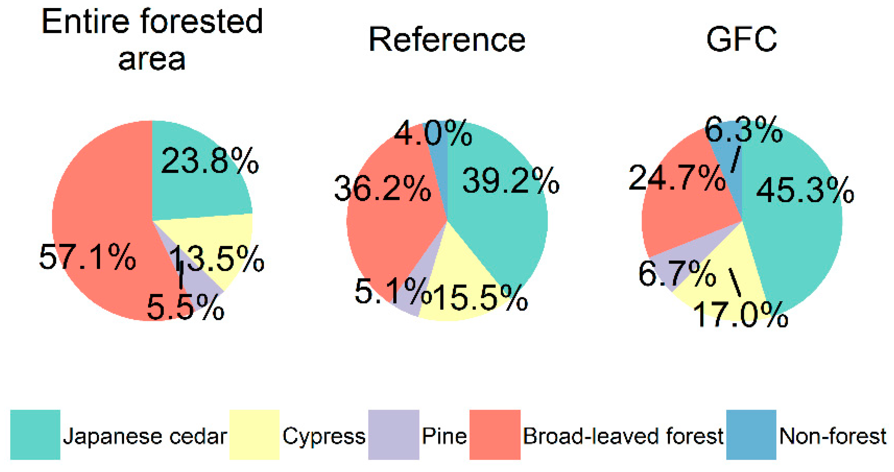
According to both the reference and GFC datasets, the proportions of the losses of Japanese cedar and cypress forest from 2014 to 2016 were considerably higher than their proportions in the entire forested area in 2014 (Figure 7). This difference is probably because these species are planted for timber production, so they are harvested more often than other species. The amount of broad-leaved forest loss was greater in the reference dataset than in the GFC dataset, which suggests that pre-existing forest species might influence the performance of the GFC dataset for detection of forest loss.
3.2. Recall and Precision Ratios
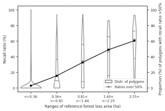
Only 11.1% of the reference forest-loss polygons had recall ratios >50%, indicating that forest loss in our study area would be under-reported on the basis of the GFC dataset. The polygons of the reference dataset with recall ratios <50% amounted to 488.3 ha, whereas those with recall ratios >50% amounted to only 291.8 ha. However, forest losses were more successfully detected in the larger polygons (Figure 8). Of the forest losses with areas >2.25 ha, 60.4% had recall ratios higher than 50%. These results suggest that many of the small forest-loss polygons were not detected in the GFC dataset. The predominance of recall ratios <50% for all reference polygons of <2.25 ha area indicates that other factors might have affected the recall ratios obtained.
Our results for precision ratio presented higher accuracies. Of the forest-loss polygons from the GFC dataset, 57.3% had precision ratios >50%. Precision ratio improved with increasing polygon area, in particular in the uppermost two ranges of polygon size (Figure 9). In the lowest size range (<0.36 ha), 49.5% of GFC polygons had precision ratios >50%, but in the highest size range (>2.25 ha), 96.6% had precision ratios >50%. As was the case for recall ratio, the distributions of precision ratio demonstrated that larger GFC polygons returned better results. Success in the identification of forest loss from the GFC dataset on the basis of precision ratio was clearly superior to that measured by recall ratio, particularly for larger areas of forest loss. However, the greater predominance of smaller polygons in the GFC dataset compared to the reference dataset (Figure 5) may have compromised the overall results of detection of forest loss from the GFC data.
3.3. Inferences on a Structural Relationship
The relationship structure determined by our application of the DirectLiNGAM algorithm indicates that area of forest loss, DCM, and tree species directly affected the recall ratios we obtained (Figure 10). As noted in the preceding section, we showed that larger areas of forest loss were better identified by the GFC dataset. Higher mean DCM values and sharper crown forms also had positive effects on recall ratio. These results indicate that forest losses that provided large amounts of timber (i.e., large areas with high DCM) from major forestry species (Japanese cedar and Japanese cypress) were more easily detected in the GFC dataset. Slope had no immediate relationship with recall ratio in our study area, although both area of forest loss and DCM showed positive associations with slope. These associations can possibly be explained in terms of the profitability of forestry operations. If both the area of harvestable timber and the height of the canopy (DCM) were large, harvesting of forest stands might be economically viable even on relatively steep slopes.
4. Discussion
Our aim was to examine the accuracy of the use of the GFC dataset [17] to identify areas of forest loss. Because many past analyses of the accuracy of land-cover maps have been done using a probability sampling approach [35,36], assessment methods based only on selected samples have been extensively developed and applied [27]. In contrast, we used a polygon-based forest-wide assessment approach. In particular, we aimed to analyze the effectiveness of the use of the GFC data to identify forest loss in a forest region with a substantial number of small forest plots, where we could assess the resolution of small polygonal areas of forest loss in the GFC dataset. Such a polygon-based analysis has practical advantages for users of the GFC dataset who require forest management at the forest-stand scale, such as the owners of the small forest plots in our study area. The availability of maps that satisfy specific users’ requirements will contribute to sustainable forest management [27,37].
The accuracies of our results were considerably lower than those of previous analyses (e.g., accuracies of 83.8% in [25] and 57.6% in [26] using pixel-based sampling points); we successfully detected forest loss (>50% recall ratio) for only 11.1% of our reference polygons. However, we achieved greater accuracy for the larger reference polygons. Thus, we infer the presence of a considerable number of small forest-loss polygons to be the reason for the poorer overall performance of our approach. Linke et al. [28] also reported that the accuracy of the GFC dataset was low for forest-loss polygons of <2 ha. These observations are consistent with the generally accepted view that patch area has a strong influence on the accuracy of interpretations of satellite imagery (e.g., [38,39]).
The results of our inference modelling on a structural relationship suggest that area of forest loss, tree species, and the height of the forest canopy are the major influences on accuracy of detection of forest loss. Previous studies have investigated the importance of geographic [40,41,42] and other forest characteristics [43] on the accuracy of land classification based on satellite imagery. However, there has been little research on the causal relations between interpretation accuracy and forest conditions. Gislason et al. [41] reported that geographic features are an important influence on interpretation accuracy, but demonstrated no immediate relationship between terrain slope and accuracy in this study. Although at first glance the difference of the distributions of slope in the reference and GFC datasets (Figure 4) seems to suggest that slope would affect accuracy, we found no immediate relationship. The relationships that we identified of slope with both polygon area and DCM might have led to this pseudo correlation (Figure 8). Clearly, understanding a structure of relationships is important for meaningful assessment of the utility of our method for application in other regions. Inferences on structural relationships are also needed for the design of sampling to avoid biases that might lead to erroneous estimations of forest loss [44]. Indeed, our results showed the benefits of modelling by revealing the unsatisfactory performance of the GFC dataset in areas of small forest plots.
5. Conclusions
We examined the accuracy of results obtained by using the GFC dataset to identify forest loss in a region with numerous small privately owned forest plots. Generally in such regions, areas of forest loss are also small. Our results indicate that use of the GFC dataset did not lead to accurate detection of areas of forest loss in our study area, and that the small size of those areas was the major factor of the inaccuracy. These results imply that forest conditions in a particular region inevitably affect the accuracy of the use of satellite imagery to detect forest loss. If satellite images are used for this purpose, the causal relationships between forest loss and the particular characteristics of that region must be considered. To support accurate application of satellite imagery for future regional-scale sustainable forest management, further studies are required to examine the causal relationships between accuracy of land-use classification and different forest conditions in various regions.
Author Contributions
Conceptualization, Y.Y.; methodology, Y.Y. and T.O.; software, Y.Y.; validation, Y.Y., T.O. and K.S.; formal analysis, Y.Y.; investigation, Y.Y.; resources, T.O. and Y.Y.; data curation, T.O. and Y.Y.; writing—original draft preparation, Y.Y.; writing—review and editing, K.S.; visualization, Y.Y.; supervision, Y.Y. and K.S.; project administration, Y.Y.; funding acquisition, Y.Y. All authors have read and agreed to the published version of the manuscript.
Funding
This research was funded by the Japan Society for the Promotion of Science KAKENHI Grant Number JP 19K15878.
Acknowledgments
We thank Oita prefectural government and Bungo-Ono municipal government for providing data used in this study.
Conflicts of Interest
The authors declare no conflict of interest.
References
- Chazdon, R.L. Beyond deforestation: Restoring forests and ecosystem services on degraded lands. Science 2008, 320, 1458–1460. [Google Scholar] [CrossRef] [PubMed] [Green Version]
- Fahrig, L. Effects of Habitat Fragmentation on Biodiversity. Annu. Rev. Ecol. Evol. Syst. 2003, 34, 487–515. [Google Scholar] [CrossRef] [Green Version]
- Holl, K.D.; Aide, T.M. When and where to actively restore ecosystems? For. Ecol. Manag. 2011, 261, 1558–1563. [Google Scholar] [CrossRef]
- Harris, N.L.; Goldman, E.; Gabris, C.; Nordling, J.; Minnemeyer, S.; Ansari, S.; Lippmann, M.; Bennett, L.; Raad, M.; Hansen, M.; et al. Using spatial statistics to identify emerging hot spots of forest loss. Environ. Res. Lett. 2017, 12, 024012. [Google Scholar] [CrossRef]
- Alvarenga, L.D.P.; Pôrto, K.C.; de Oliveira, J.R.d.P.M. Habitat loss effects on spatial distribution of non-vascular epiphytes in a Brazilian Atlantic forest. Biodivers. Conserv. 2010, 19, 619–635. [Google Scholar] [CrossRef]
- Lowrance, R.; Todd, R.; Fail, J.; Hendrickson, O.; Leonard, R.; Asmussen, L. Riparian Forests as Nutrient Filters in Agricultural Watersheds. Bioscience 1984, 34, 374–377. [Google Scholar] [CrossRef]
- Gregory, S.V.; Swanson, F.J.; McKee, W.A.; Cummins, K.W. An Ecosystem Perspective of Riparian Zones. Bioscience 1991, 41, 540–551. [Google Scholar] [CrossRef]
- Allan, J.D. Landscapes and Riverscapes: The Influence of Land Use on Stream Ecosystems. Annu. Rev. Ecol. Evol. Syst. 2004, 35, 257–284. [Google Scholar] [CrossRef] [Green Version]
- Blumenthal, S.A.; Chritz, K.L.; Rothman, J.M.; Cerling, T.E. Detecting intraannual dietary variability in wild mountain gorillas by stable isotope analysis of feces. Proc. Natl. Acad. Sci. USA 2012, 109, 21277–21282. [Google Scholar] [CrossRef] [Green Version]
- Zurita, G.A.; Bellocq, M.I. Spatial patterns of bird community similarity: Bird responses to landscape composition and configuration in the Atlantic forest. Landsc. Ecol. 2010, 25, 147–158. [Google Scholar] [CrossRef]
- Yamada, Y. Can a regional-level forest management policy achieve sustainable forest management? For. Policy Econ. 2018, 90, 82–89. [Google Scholar] [CrossRef]
- Yamada, Y.; Yamaura, Y. Decision Support System for Adaptive Regional-Scale Forest Management by Multiple Decision-Makers. Forests 2017, 8, 453. [Google Scholar] [CrossRef] [Green Version]
- Voigt, S.; Kemper, T.; Riedlinger, T.; Kiefl, R.; Scholte, K.; Mehl, H. Satellite image analysis for disaster and crisis-management support. IEEE Trans. Geosci. Remote Sens. 2007, 45, 1520–1528. [Google Scholar] [CrossRef]
- Kennedy, R.E.; Yang, Z.; Cohen, W.B.; Pfaff, E.; Braaten, J.; Nelson, P. Spatial and temporal patterns of forest disturbance and regrowth within the area of the Northwest Forest Plan. Remote Sens. Environ. 2012, 122, 117–133. [Google Scholar] [CrossRef]
- Wilson, E.H.; Sader, S.A. Detection of forest harvest type using multiple dates of Landsat TM imagery. Remote Sens. Environ. 2002, 80, 385–396. [Google Scholar] [CrossRef]
- Potapov, P.; Hansen, M.C.; Kommareddy, I.; Kommareddy, A.; Turubanova, S.; Pickens, A.; Adusei, B.; Tyukavina, A.; Ying, Q. Landsat Analysis Ready Data for Global Land Cover and Land Cover Change Mapping. Remote Sens. 2020, 12, 426. [Google Scholar] [CrossRef] [Green Version]
- Hansen, M.C.; Potapov, P.V.; Moore, R.; Hancher, M.; Turubanova, S.A.; Thau, D.; Stehman, S.V.; Goetz, S.J.; Loveland, T.R.; Kommareddy, A.; et al. High-resolution global maps of 21st-century forest cover change. Science 2013, 342, 850–853. [Google Scholar] [CrossRef] [Green Version]
- Brandt, J.S.; Nolte, C.; Agrawal, A. Deforestation and timber production in Congo after implementation of sustainable forest management policy. Land Use Policy 2016, 52, 15–22. [Google Scholar] [CrossRef]
- Chazdon, R.L.; Broadbent, E.N.; Rozendaal, D.M.A.; Bongers, F.; Zambrano, A.M.A.; Aide, T.M.; Balvanera, P.; Becknell, J.M.; Boukili, V.; Brancalion, P.H.S.; et al. Carbon sequestration potential of second-growth forest regeneration in the Latin American tropics. Sci. Adv. 2016, 2, e1501639. [Google Scholar] [CrossRef] [Green Version]
- Oldekop, J.A.; Sims, K.R.E.; Karna, B.K.; Whittingham, M.J.; Agrawal, A. Reductions in deforestation and poverty from decentralized forest management in Nepal. Nat. Sustain. 2019, 2, 421–428. [Google Scholar] [CrossRef] [Green Version]
- Santika, T.; Wilson, K.A.; Budiharta, S.; Kusworo, A.; Meijaard, E.; Law, E.A.; Friedman, R.; Hutabarat, J.A.; Indrawan, T.P.; St. John, F.A.V.; et al. Heterogeneous impacts of community forestry on forest conservation and poverty alleviation: Evidence from Indonesia. People Nat. 2019, 1, pan3.25. [Google Scholar] [CrossRef]
- Taylor, C.M.; Stutchbury, B.J.M. Effects of breeding versus winter habitat loss and fragmentation on the population dynamics of a migratory songbird. Ecol. Appl. 2016, 26, 424–437. [Google Scholar] [CrossRef] [PubMed]
- Wall, J.; Wittemyer, G.; Klinkenberg, B.; Douglas-Hamilton, I. Novel opportunities for wildlife conservation and research with real-time monitoring. Ecol. Appl. 2014, 24, 593–601. [Google Scholar] [CrossRef] [PubMed] [Green Version]
- Stoffels, J.; Hill, J.; Sachtleber, T.; Mader, S.; Buddenbaum, H.; Stern, O.; Langshausen, J.; Dietz, J.; Ontrup, G. Satellite-Based Derivation of High-Resolution Forest Information Layers for Operational Forest Management. Forests 2015, 6, 1982–2013. [Google Scholar] [CrossRef]
- Arjasakusuma, S.; Kamal, M.; Hafizt, M.; Forestriko, H.F. Local-scale accuracy assessment of vegetation cover change maps derived from Global Forest Change data, ClasLite, and supervised classifications: Case study at part of Riau Province, Indonesia. Appl. Geomat. 2018, 10, 205–217. [Google Scholar] [CrossRef]
- Milodowski, D.T.; Mitchard, E.T.A.; Williams, M. Forest loss maps from regional satellite monitoring systematically underestimate deforestation in two rapidly changing parts of the Amazon. Environ. Res. Lett. 2017, 12, 094003. [Google Scholar] [CrossRef] [Green Version]
- Stehman, S.V.; Wickham, J.D. Pixels, blocks of pixels, and polygons: Choosing a spatial unit for thematic accuracy assessment. Remote Sens. Environ. 2011, 115, 3044–3055. [Google Scholar] [CrossRef]
- Linke, J.; Fortin, M.-J.; Courtenay, S.; Cormier, R. High-resolution global maps of 21st-century annual forest loss: Independent accuracy assessment and application in a temperate forest region of Atlantic Canada. Remote Sens. Environ. 2017, 188, 164–176. [Google Scholar] [CrossRef]
- Shimizu, S.; Hoyer, P.O.; Hyvärinen, A.; Kerminen, A. A linear non-gaussian acyclic model for causal discovery. J. Mach. Learn. Res. 2006, 7, 2003–2030. [Google Scholar]
- Shimizu, S. Lingam: Non-Gaussian Methods for Estimating Causal Structures. Behaviormetrika 2014, 41, 65–98. [Google Scholar] [CrossRef]
- Lanka, S.; Shimizu, S.; Inazumi, T.; Sogawa, Y.; Hyvärinen, A.; Kawahara, Y.; Washio, T.; Hoyer, P.O.; Bollen, K. DirectLiNGAM: A direct method for learning a linear non-Gaussian structural equation model. J. Mach. Learn. Res. 2011, 12, 1225–1248. [Google Scholar]
- Sharma, R.; Hara, K.; Tateishi, R. High-Resolution Vegetation Mapping in Japan by Combining Sentinel-2 and Landsat 8 Based Multi-Temporal Datasets through Machine Learning and Cross-Validation Approach. Land 2017, 6, 50. [Google Scholar] [CrossRef] [Green Version]
- Ota, T.; Mizoue, N.; Yoshida, S. Influence of using texture information in remote sensed data on the accuracy of forest type classification at different levels of spatial resolution. J. For. Res. 2011, 16, 432–437. [Google Scholar] [CrossRef]
- Tanaka, S.; Takahashi, T.; Saito, H.; Awaya, Y.; Iehara, T.; Matsumoto, M.; Sakai, T. Simple Method for Land-Cover Mapping by Combining Multi-Temporal Landsat ETM+ Images and Systematically Sampled Ground Truth Data: A Case Study in Japan. J. For. Plan. 2012, 18, 77–85. [Google Scholar] [CrossRef]
- Olofsson, P.; Foody, G.M.; Herold, M.; Stehman, S.V.; Woodcock, C.E.; Wulder, M.A. Good practices for estimating area and assessing accuracy of land change. Remote Sens. Environ. 2014, 148, 42–57. [Google Scholar] [CrossRef]
- Strahler, A.H.; Boschetti, L.; Foody, G.M.; Friedl, M.A.; Hansen, M.C.; Herold, M.; Mayaux, P.; Morisette, J.T.; Stehman, S.V.; Woodcock, C.E. Global Land Cover Validation: Recommendations for Evaluation and Accuracy Assessment of Global land Cover Maps; EUR 22156 EN–DG; Office for Official Publications of the European Communities: Luxemburg, 2006. [Google Scholar]
- Corbane, C.; Carrion, D.; Broglia, M. Development and implementation of a validation protocol for crisis maps: Reliability and consistency assessment of burnt area maps. Int. J. Digit. Earth 2011, 4, 8–24. [Google Scholar] [CrossRef]
- Baumann, M.; Ozdogan, M.; Wolter, P.T.; Krylov, A.; Vladimirova, N.; Radeloff, V.C. Landsat remote sensing of forest windfall disturbance. Remote Sens. Environ. 2014, 143, 171–179. [Google Scholar] [CrossRef]
- Jin, S.; Sader, S.A. MODIS time-series imagery for forest disturbance detection and quantification of patch size effects. Remote Sens. Environ. 2005, 99, 462–470. [Google Scholar] [CrossRef]
- Belgiu, M.; Drăgu, L. Random forest in remote sensing: A review of applications and future directions. Isprs J. Photogramm. Remote Sens. 2016, 114, 24–31. [Google Scholar] [CrossRef]
- Gislason, P.O.; Benediktsson, J.A.; Sveinsson, J.R. Random forests for land cover classification. Pattern Recognit. Lett. 2006, 27, 294–300. [Google Scholar] [CrossRef]
- Corcoran, J.; Knight, J.; Gallant, A. Influence of Multi-Source and Multi-Temporal Remotely Sensed and Ancillary Data on the Accuracy of Random Forest Classification of Wetlands in Northern Minnesota. Remote Sens. 2013, 5, 3212–3238. [Google Scholar] [CrossRef] [Green Version]
- McRoberts, R.E.; Vibrans, A.C.; Sannier, C.; Næsset, E.; Hansen, M.C.; Walters, B.F.; Lingner, D.V. Methods for evaluating the utilities of local and global maps for increasing the precision of estimates of subtropical forest area. Can. J. For. Res. 2016, 46, 924–932. [Google Scholar] [CrossRef] [Green Version]
- Stehman, S.V.; Foody, G.M. Key issues in rigorous accuracy assessment of land cover products. Remote Sens. Environ. 2019, 231, 111199. [Google Scholar] [CrossRef]
Figure 1.
(a,b) Location map and (c) forest type distribution map of the study area. Forest type distribution was visually interpreted from the aerial photographs acquired in 2014.
Figure 1.
(a,b) Location map and (c) forest type distribution map of the study area. Forest type distribution was visually interpreted from the aerial photographs acquired in 2014.

Figure 2.
Examples of forest-loss polygons of (a,b) the reference dataset and (c,d) the GFC dataset with the Landsat composite images in (a,c) 2014 and (b,d) 2017 that cover between June 2014 and December 2016. The Landsat composite images were used only for visualization.
Figure 2.
Examples of forest-loss polygons of (a,b) the reference dataset and (c,d) the GFC dataset with the Landsat composite images in (a,c) 2014 and (b,d) 2017 that cover between June 2014 and December 2016. The Landsat composite images were used only for visualization.

Figure 3.
Schematic illustration of a forest-loss polygon including non-forest. Four percent of the forest-loss polygon in this figure is covered with non-forest with lower resolution land classification map.
Figure 3.
Schematic illustration of a forest-loss polygon including non-forest. Four percent of the forest-loss polygon in this figure is covered with non-forest with lower resolution land classification map.

Figure 4.
Schematic illustration of method for calculation of recall and precision ratios.

Figure 5.
Comparison of violin and box plots of the distributions of areas of forest loss during 2014 to 2016 derived from the GFC and reference datasets.
Figure 5.
Comparison of violin and box plots of the distributions of areas of forest loss during 2014 to 2016 derived from the GFC and reference datasets.

Figure 6.
Comparison of violin and box plots of the distribution of slope for the entire forested part of the study area with the distributions for areas of forest loss during 2014 to 2016 derived from the reference and GFC datasets.
Figure 6.
Comparison of violin and box plots of the distribution of slope for the entire forested part of the study area with the distributions for areas of forest loss during 2014 to 2016 derived from the reference and GFC datasets.

Figure 7.
Comparison of the proportions of forest type in the entire forested part of the study area in 2014 (reference dataset) with those in areas of forest loss from 2014 to 2016 derived from the GFC and reference datasets.
Figure 7.
Comparison of the proportions of forest type in the entire forested part of the study area in 2014 (reference dataset) with those in areas of forest loss from 2014 to 2016 derived from the GFC and reference datasets.

Figure 8.
Comparison of violin plots of the distributions of recall ratios for forest-loss polygons in the reference dataset in five size ranges. Dashed horizontal lines show quartile and median values. For each size range, the black dots mark the proportion of forest-loss polygons successfully being detected (recall ratio >50%) in the reference dataset.

Figure 9.
Comparison of violin plots of the distributions of precision ratios for forest-loss polygons in the reference dataset in five size ranges. Dashed horizontal lines show quartile and median values. For each size range, the black dots mark the proportion of forest-loss polygons successfully detected (precision ratio >50%) in the GFC dataset.

Figure 10.
Structural relationships inferred by application of the DirectLiNGAM algorithm. The arrows show directions of influences and the numbers besides the arrows are the inferred values of coefficients () of Equation (2). Positive (negative) values indicate positive (negative) effects. Higher |B| indicates a stronger relationship.

© 2020 by the authors. Licensee MDPI, Basel, Switzerland. This article is an open access article distributed under the terms and conditions of the Creative Commons Attribution (CC BY) license (http://creativecommons.org/licenses/by/4.0/).
Share and Cite
MDPI and ACS Style
Yamada, Y.; Ohkubo, T.; Shimizu, K. Causal Analysis of Accuracy Obtained Using High-Resolution Global Forest Change Data to Identify Forest Loss in Small Forest Plots. Remote Sens. 2020, 12, 2489. https://doi.org/10.3390/rs12152489
AMA Style
Yamada Y, Ohkubo T, Shimizu K. Causal Analysis of Accuracy Obtained Using High-Resolution Global Forest Change Data to Identify Forest Loss in Small Forest Plots. Remote Sensing. 2020; 12(15):2489. https://doi.org/10.3390/rs12152489
Chicago/Turabian StyleYamada, Yusuke, Toshihiro Ohkubo, and Katsuto Shimizu. 2020. "Causal Analysis of Accuracy Obtained Using High-Resolution Global Forest Change Data to Identify Forest Loss in Small Forest Plots" Remote Sensing 12, no. 15: 2489. https://doi.org/10.3390/rs12152489
Note that from the first issue of 2016, this journal uses article numbers instead of page numbers. See further details here.