Classification of Hyperspectral Reflectance Images With Physical and Statistical Criteria

Abstract

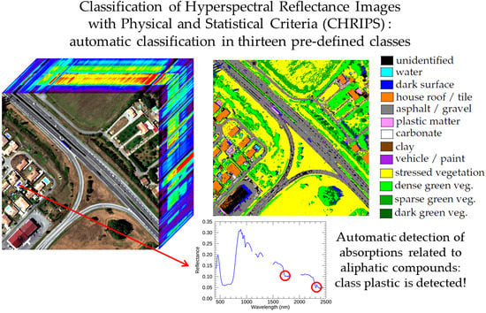
A classification method of hyperspectral reflectance images named CHRIPS (Classification of Hyperspectral Reflectance Images with Physical and Statistical criteria) is presented. This method aims at classifying each pixel from a given set of thirteen classes: unidentified dark surface, water, plastic matter, carbonate, clay, vegetation (dark green, dense green, sparse green, stressed), house roof/tile, asphalt, vehicle/paint/metal surface and non-carbonated gravel. Each class is characterized by physical criteria (detection of specific absorptions or shape features) or statistical criteria (use of dedicated spectral indices) over spectral reflectance. CHRIPS input is a hyperspectral reflectance image covering the spectral range [400–2500 nm]. The presented method has four advantages, namely: (i) is robust in transfer, class identification is based on criteria that are not very sensitive to sensor type; (ii) does not require training, criteria are pre-defined; (iii) includes a reject class, this class reduces misclassifications; (iv) high precision and recall, F${}_1$ score is generally above 0.9 in our test. As the number of classes is limited, CHRIPS could be used in combination with other classification algorithms able to process the reject class in order to decrease the number of unclassified pixels.

1. Introduction

Hyperspectral remote sensing allows the simultaneous acquisition of hundreds of narrow and contiguous spectral bands usually ranging from the visible to the short-wave infrared (SWIR). The pixel spectra provided by such sensors are functions of the solar irradiation, the atmospheric effects (absorption and diffusion by molecules and particles), the interaction of radiation with the ground and the transfer function of the instrument. They can thus be exploited to extract information about the components of the studied scene (material constituents, gaseous and aerosol concentrations) from the modeling of the interaction between the electromagnetic radiation and the medium.

In this paper, we focus on the classification problematic for hyperspectral images. This topic has been the subject of numerous studies in recent years and led to the development of many unsupervised and supervised classification methods [1]. Unsupervised algorithms mainly gather centroid-based clustering methods [2,3], density-based methods [4,5], biological clustering methods [6,7] and graph-based methods [8,9,10].

Supervised methods can be separated into two groups—methods using metrics and machine learning methods. Methods using metrics, such as Spectral Angle Mapper (SAM) and Spectral Information Divergence (SID) [11,12,13], aim to match pixel spectra with a spectral database or learning samples. Machine learning algorithms have been studied a lot for hyperspectral classification. Many pixelwise classification methods exploiting only the spectral dimension were proposed, such as maximum likelihood [14], neural networks [15], random forest [16], multinomial logistic regression [17] and support vector machines [18]. Several approaches were developed to exploit both spectral and spatial information: extended morphological profiles [19,20], composite kernel [21], morphological kernel [22,23]. Recently, many deep learning methods were developed and achieved good performance [24,25]. Some of them are purely spectral [26,27,28,29,30] and others exploit both spectral and spatial dimensions [31,32,33].

Besides, software such as TetraCorder [34] and Hysoma [35] allows the detection and the characterization of physical features by computing some criteria dedicated to different types of surfaces and materials. Such software could also be used for classification.

Some methods aim at characterizing specific types of surface based on spectral criteria by the mean of dedicated indices. For instance, green vegetation can be detected with NDVI (Normalized Difference Vegetation Index) due to plant photosynthesis [36,37], or CAI (Cellulose Absorption Index) can detect senescent or mixture of vegetation/bare soils [38,39]. For natural bare soils, Hysoma [35] can be used to assess soil, humidity, clay, carbonate contents, and so forth. Some spectral indices have also been defined for impervious surface [40,41]—they are used to map urban areas mainly from satellite images. But all these indices are used to assess specific surfaces and generally require thresholding from user, which may be a tricky task.

Spectral reflectance is a very useful tool to characterize surfaces. Even if atmospheric effects still can be observed as they are never perfectly removed by atmospheric correction, and illumination may introduce a scaling on spectra, reflectance depends much less on atmospheric conditions and illumination than spectral radiance. Reflectance may exhibit specific features at some spectral bands that could give crucial information on material components (see Figure 1).

These features can be observed whatever the hyperspectral sensor as long as it contains the appropriate spectral bands. Some robust criteria could then be built in order to identify them: this is the purpose of the new classification method CHRIPS (Classification of Hyperspectral Reflectance Images with Physical and Statistical criteria) that is presented in this paper. This method considers the main surface types commonly present on land remote sensing images. It defines some discriminant criteria dedicated to each class. These criteria exploit physical and statistical features that may be observed on spectral reflectance. CHRIPS aims at reaching two main objectives.

• The first objective is to perform a classification without using any expert knowledge from user. For unsupervised methods, the selection of the number of classes is not straightforward even if some methods try to estimate it [42,43]. Methods using metrics (SAM, SID) require thresholds to be tuned—this task cannot be performed easily. For machine learning methods, training samples need to be selected for each class, but spatial location of these training samples on images is often unknown. The number of classes CHRIPS could detect is fixed. For each class, CHRIPS applies a set of criteria that depend on thresholds for which robust values were estimated once for all from training samples covering as much as possible spectral variability of each class. Then, CHRIPS only requires a hyperspectral reflectance image as input.
• The second objective is that the classification method can be applied on hyperspectral images acquired at different spectral and spatial resolutions by common airborne hyperspectral sensors. Machine learning methods may be quite accurate when the trained model is applied on images acquired with the same sensor and the same spatial resolution as the training samples, but may be less efficient when it is applied on images acquired with other sensors (transfer ability) because they are generally not trained for more than one sensor. CHRIPS method is based on the computation of criteria that are robust to the sensor change.

The paper is organized as follows. In Section 2, an overview of classification method CHRIPS is presented. Section 3 presents hyperspectral datasets used to design and assess the CHRIPS method. Section 4 presents pre-processings. In Section 5, all criteria used for the characterization of each class are defined. In Section 6, a post-processing allowing the reduction of unidentified pixels is presented. Section 7 explains how the CHRIPS method should be applied. In Section 8, CHRIPS method is assessed on several hyperspectral images acquired with three different sensors at different spatial resolutions and is compared with some widely used spectral classification methods. In Section 9, main characteristics of CHRIPS are discussed. Finally, we give conclusion and highlight the potential directions of future research work.

2. Overview of Classification Method Chrips

CHRIPS is a hierarchical classification method that can be applied on hyperspectral reflectance images covering the spectral range [400–2500 nm]. For each class, a dedicated detection method exploits specific spectral properties (specific absorptions or shape features) or spectral indices. CHRIPS method identifies thirteen different classes that are gathered into four groups: dark surfaces, materials with specific absorptions, vegetation and other types of surfaces (scattering surfaces). The class assignment is hierarchical: classes are investigated one after the other in a given order. Class order is defined by the complexity of class characterization. It allows to reduce the number of criteria that are required to characterize each class. The ordered classes are given by the following list:

• dark surface

  (1)

  dark green vegetation

  (2)

  water

  (3)

  unidentified dark surface

• material with specific absorptions

  (4)

  plastic matter (aliphatic + aromatic)

  (5)

  carbonate

  (6)

  clay

• vegetation

  (7)

  dense green vegetation

  (8)

  sparse green vegetation

  (9)

  stressed vegetation

• classes with dedicated indices

  (10)

  house roof/tile

  (11)

  asphalt

  (12)

  vehicle/paint/metal surface

  (13)

  non-carbonated gravel

• unidentified

First of all, dark surfaces are identified: they are defined as surfaces for which reflectances are very low in the SWIR range. They are also processed first because corresponding spectra are very noisy and may check sometimes criteria of other classes. Secondly, materials with specific absorptions are identified. They correspond to materials that present very local minima on spectral reflectance due to electronic or vibrational processes [44]. For instance, reflectances of surfaces containing clay have a local minimum around 2200 nm. Thirdly, vegetation classes are identified. They can be characterized with dedicated indices [45] that highlight some bio-physical properties (chlorophyll content, water content, stress, etc.) or geometric features (local maxima, etc.). In the end, the remaining classes are more complex to describe—they do not exhibit any physical or observable features that make it possible to characterize them. It is why they are processed after all other classes. We propose to compute some combinations of indices in the same way as vegetation indices and that would be dedicated to a given class.

These classes where chosen because they are often found in aerial images. Carbonate and clay classes are less common but can still be observed in surfaces such as sand, limestone paths, clay soils in agricultural fields, lithological formations, and so forth.

The classification process CHRIPS is based on a sequential tree of detection. Each class is characterized with a few criteria and classes are ordered. The process of classification is as follows. For each pixel, all criteria associated to class 1 are assessed. If all criteria are true, the pixel is considered as belonging to class 1 and the process ends. If at least one criterion is false, the pixel does not belong to class 1, criteria of class 2 are then assessed. The same process is conducted class after class. If at the end, the pixel does not belong to any of the defined classes, it is considered as unidentified.

CHRIPS includes a reject class that reduces the risk of misclassification. In general, the reject class includes spectra that do not correspond to any class of CHRIPS or correspond to mixed spectra—depending on spatial resolution, many pixels may contain different materials or surfaces and then a unique label could not be easily assigned to them (except in the case where a given class has a large majority).

At the output of the CHRIPS method, a spatial regularization step is applied to possibly assign a class to unclassified pixels. This processing is described in Section 6.

The full processing chain of CHRIPS is presented in Figure 2.

CHRIPS class criteria only use spectral information—spatial dimension is not taken into account. However, the regularization processing takes into account neighboring pixels. Otherwise, spatial features are not used by CHRIPS criteria. Many machine learning methods, notably deep learning methods, exploit spatial features and give quite accurate results. However, in practice, such spatial features are hard to gather in hyperspectral images. Intraclass spatial information is sometimes accessible but interclass spatial information is rarer. Currently, there is no database dedicated to hyperspectral remote sensing which includes a lot of annotated data and then would make possible to learn spatial features, on the contrary to many other types of images where deep learning could be more easily applied: traditional color images, medical images, and so forth. Moreover, spatial features are not very robust when changing spatial resolution: spatial characteristics at a given resolution may be false at other resolutions and then may decrease classification performances and transfer ability. Spatial features also depend on the layout of the landscape (different types of urban, semi-urban, rural landscapes, etc.), while the CHRIPS method is developed to be as insensitive as possible to this.

CHRIPS does not require exogenous data from the user—its only input is the hyperpectral reflectance image. Some classical inputs such as the selection of training samples (for supervised machine learning methods), the number of classes (for unsupervised methods) or the values of thresholds (for metric-based methods) are not required. Each CHRIPS criterion depends on thresholds for which robust values were estimated from training data and are proposed in this paper, CHRIPS application is fully unsupervised. Moreover, CHRIPS criteria are designed to work for several spectral resolutions, which make it possible to apply the method on images acquired with different sensors.

CHRIPS could be applied for very different thematic applications: change detection (comparison of classification maps between several dates), detection of plastic matter (garbage in uncontrolled landfills, ocean waste plastic, synthetic structures, boats, etc.), identification of clay surfaces (study of trafficability as clay may retain water), characterization of vegetation (agriculture, vegetation health, trafficability, etc.), characterization of urban surfaces (roads, roofs, vehicles), and so forth. It could also be used in the search for hydrocarbons (onshore oil spill, pipeline leak, etc.) as oil has the same absorptions as plastic and could be detected with the same criteria.

3. Datasets

3.1. Presentation of Hyperspectral Datasets

Eleven hyperspectral images acquired with four different sensors are used. These images are used for the design of CHRIPS criteria (training) and for validation (test):

• five Odin images (training),
• two HySpex images: Fauga (training) and Mauzac (test),
• one HyMap image: Garons (test),
• three AisaFENIX images: surburban Mauzac (test).

Characteristics of these images are shown in

Table 1. Characteristics of hyperspectral images used in this paper: sensor used for acquisition, number N${}_{\mathrm{I}}$ of images, number N${}_{\mathrm{S}}$ of spectral bands, mean value of full width at half maximum (FHWM) in VNIR and SWIR ranges and spatial resolution.

			FWHM	FWHM	Spatial
Sensor	N${}_{\mathbf{I}}$	N${}_{\mathbf{S}}$	VNIR	SWIR	Resolution
HySpex	2	416	4 nm	6 nm	0.3 m
HyMap	1	125	15 nm	15 nm	4 m
Odin	5	426	4 nm	9 nm	0.5 m
AisaFENIX	3	420	3.5 nm	7.5 nm	0.55/2.2/8.8 m

. False color of all HySpex, HyMap and AisaFENIX images are represented in Figure 3.

3.1.1. Odin Images

Five hyperspectral images were acquired close to Toulon (France) with the Odin hyperspectral sensor (Norsk Elektro Optikk) within the context of the Sysiphe Step 2 project, managed and funded by the DGA. The Odin sensor provides 426 bands with a covering spectral coverage ranging between 423 nm and 2507 nm. The spatial resolution is 0.5 m. These images cover very different landscapes: forest, sea, beach, urban area, parking lot, airport, harbour, and so forth.

3.1.2. HySpex Images

Two images of Fauga and Mauzac (France) were acquired by ONERA (Office National d’Etudes et de Recherches Aérospatiales, The French Aerospace Lab) with the HySpex hyperspectral sensor (Norsk Elektro Optikk [46]) within the context of the Hypex project, managed and funded by the DGA (Direction Générale de l’Armement). The HySpex sensor is composed of two cameras—a VNIR camera and a SWIR camera. The VNIR camera (VNIR-1600) provides 160 bands with a spectral coverage ranging from 415 nm to 992 nm. The SWIR camera (SWIR-320m) provides 256 bands with a spectral coverage ranging from 967 nm to 2500 nm. Spatial resolution was 0.3 m for VNIR images and 0.6 m for SWIR images. SWIR images were oversampled at 0.3 m and registered on VNIR images in order to obtain hyperspectral images covering the spectral range [415–2500 nm] with the same spatial resolution. Both images cover parts of the villages of Fauga and Mauzac, South-West of France. They gather vegetation (trees, grass), houses, road, limestone paths, vehicles, plastic matter (tarpaulin, canopy/pergola, garbage bags, etc.).

3.1.3. HyMap Image

The HyMap sensor provides 125 bands with a spectral coverage ranging between 454 nm and 2496 nm. A hyperspectral image was acquired over the agricultural site of Garons (France) in August 2009. The flight was operated by the Deutschen Zentrum für Luft- und Raumfahrt (DLR, German Aerospace Agency) during an ONERA campaign. The spatial resolution is 4 m per pixel. This image gathers several vegetation types and cultures: vineyards, orchards (peach, kiwi, apricot), market gardening (zucchini), meadows, forest, clay soils. It also contains greenhouses (plastic matter), roads, limestone paths, rivers and sparse houses.

3.1.4. AisaFENIX Images

A hyperspectral image was acquired by ONERA over a suburban area of Mauzac, a village in South-West of France, with the AisaFENIX sensor (Specim, Spectral Imaging Ltd, http://www.specim.fi). The AisaFENIX sensor provides 420 bands in the spectral range [382–2502 nm]. In order to assess the impact of spatial resolution on classification performances, three hyperspectral images of a suburban area of Mauzac (France) with different spatial resolutions are considered: 0.55 m, 2.2 m and 8.8 m. For convenience, images are denoted $I_{0.55}$, $I_{2.2}$ and $I_{8.8}$ and corresponding ground truth are denoted $G_{0.55}$, $G_{2.2}$ and $G_{8.8}$ (see Section 3.3 for details on the process of creating the ground truth). The image $I_{0.55}$ was acquired with the hyperspectral sensor AisaFENIX. Images $I_{2.2}$ and $I_{8.8}$ were simulated using a dedicated processing chain [47]. A first atmospheric correction is applied to airborne radiance using the COCHISE code (atmospheric COrrection Code for Hyperspectral Images of remote SEnsing sensors [48,49]). COCHISE retrieves the surface spectral reflectance as well as the water vapor content from a sensor-level radiance image. It removes atmospheric and environment effects. The atmospheric radiative parameters are computed using MODTRAN 5 [50]. Spectral reflectances are resampled to the same spectral resolution (3.5 nm in VNIR and 7.5 nm in SWIR). Then, satellite simulated radiance is computed with the Comanche code [48]. Spatial aggregation, noise and point spread function are applied following the specifications of the future hyperspectral satellite Hypxim [51]. Finally, reflectance spectra are retrieved using COCHISE.

3.2. Selection of Training Samples

CHRIPS method sorts the pixels into thirteen different classes as described in Section 2. For each class, criteria are defined from a set $S_{\rho }^1$ of reflectance spectra that are used as training samples: $S_{\rho }^1$ gathers around 9500 reflectance spectra. These training samples are extracted from a dataset $S_I$ composed of the six following hyperspectral images: Fauga (HySpex) and five Odin images (more details in Section 3.1) that were interpolated at HySpex spectral bands (spectral resolution of 4–6 nm).

These samples aim to cover as much spectral variability as possible for each class and to allow the design of criteria that are as robust as possible. The sample collection has been enriched several times by iterating the following process:

–

design of optimal CHRIPS criteria from the training samples $S_{\rho }^1$ (see Section 5)

–

application of CHRIPS on the set of images $S_I$

–

identification of misclassified pixels

–

update of $S_{\rho }^1$: addition of new training samples from misclassified pixels

Depending on the spectral variability of each class and the discriminating power of CHRIPS criteria, the number of training samples varies from class to class: dark green vegetation (240 spectra), water(400) unidentified dark surface (350), plastic matter (aliphatic and aromatic: 510), carbonate (250), clay (210), dense green vegetation (630), sparse green vegetation (660), stressed vegetation (940), house roof/tile (1230), asphalt (800), vehicle (3030), non-carbonated gravel (250).

Spectral resolution of sensors may have an impact on criteria robustness, especially for classes with specific absorption bands. Indeed, depth of absorption bands may be reduced for spectral resolutions higher than HySpex and then thresholds may vary depending on spectral resolution. All spectral reflectances from $S_{\rho }^1$ are downsampled at HyMap spectral resolution (15 nm) and then resampled at HySpex resolution (4–6 nm): these resampled spectra are gathered in a set denoted $S_{\rho }^2$. The final set of training samples $S_{\rho }$ is obtained by bringing together $S_{\rho }^1$ and $S_{\rho }^2$ (19,000 spectra). This process allows to take into account reflectance spectra at HySpex spectral resolution as well as smooth reflectance spectra acquired with sensors having a lower resolution than HySpex during the process of threshold estimation (see Section 5.1).

It was preferred to use spectral reflectances acquired from images as training samples, even though they may be contaminated by errors due to imperfect atmospheric correction, rather than ground measurements. Indeed, ground measurements raise the problem of scaling when they are transposed to airborne data. Local measurements need to be aggregated taking into account many parameters such as the three-dimensional structure of materials, the spectral variability and spatial distribution of its constituents, and so forth. Modelling remote sensing spectra is then a very complex task that varies from class to class and may introduce inaccuracies. In addition, spectral variability is easier to take into account with spectra extracted from images than with ground samples alone.

Quality of reflectance spectra acquired from hyperspectral images highly depends on radiometric correction and atmospheric correction. These processings were carried out carefully for all images from dataset $S_I$. Radiometric calibration based on laboratory measurements is supplemented by an in-flight calibration correction using reference panels placed on the flight line.

3.3. Images and Ground Truth Used for Assessment

Some classical images such as Pavia University and Pavia Center are often used to assess classification algorithms. However, these images were acquired with the Reflective Optics System Imaging Spectrometer (ROSIS-03) optical sensor and have a spectral coverage ranging from 430 to 860 nm. The CHRIPS method mainly uses SWIR spectral bands and then cannot be applied to these images. Another often used image is the agricultural Indian Pine test site (Indiana, USA) acquired with the Airborne Visible/Infrared Imaging Spectrometer (AVIRIS). Ground truth in this image only focuses on vegetation and is not suitable for the assessment of CHRIPS. The following hyperspectral images are used for assessment:

• Fauga (HySpex)
• Mauzac (HySpex)
• Garons (HyMap)
• suburban Mauzac (AisaFENIX): images $I_{0.55}$ (0.55 m), $I_{2.2}$ (2.2 m) and $I_{8.8}$ (8.8 m)

Further details on images are provided in Section 3.1. Some training samples come from the Fauga image. No training samples are extracted from Mauzac, Garons and surburban Mauzac images.

Campaigns were conducted to collect ground truth for all these images (measurements of reflectance spectra and visual recognition). For each image, a ground truth map was initialized by combining classification maps of CHRIPS and two other methods that are also used for assessment (SVM [18] and CNN-1D [26], see Section 8.1) with a majority vote. This ground truth map was then modified by using in situ knowledge (around 80% of ground truth was seen during campaigns) and visual inspection over hyperspectral images. Reflectance spectra are also used to suppress doubtful areas, especially for plastic, clay soils and carbonated surfaces.

For the images on suburban Mauzac, ground truth map $G_{0.55}$ is established from $I_{0.55}$. Ground truth maps $G_{2.2}$ and $G_{8.8}$ are obtained by downsampling $G_{0.55}$. Each pixel of $G_{2.2}$ is associated to $4^2=16$ pixels in $G_{0.55}$. Each pixel of $G_{8.8}$ is associated to ${16}^2=256$ pixels in $G_{0.55}$. As pixels in image $I_{2.2}$ may contain several classes, each pixel from ground truth $G_{2.2}$ is assigned the majority class among $G_{0.55}$ pixels associated to this pixel if this one exceeds 50%, and the unidentified class otherwise. The same process is applied to compute $G_{8.8}$.

4. Pre-Processing: Correction of Spectral Data

Three pre-processings are applied to each airborne hyperspectral image presented in Section 3.1: atmospheric correction, noise reduction and spectral interpolation. They also need to be applied on every hyperspectral image for which CHRIPS method is applied.

4.1. Atmospheric Correction

Reflectance can be estimated from hyperspectral radiance images by applying atmospheric correction methods based on radiative transfer codes [48,52,53,54,55,56]. In this paper, all HySpex, Odin and AisaFENIX hyperspectral images were corrected with the COCHISE code [48]. The Garons image (HyMap sensor) was corrected by the DLR. As some noise may be present on reflectance spectra after atmospheric correction, a smoothing processing is proposed in next section to reduce its effects.

4.2. Smoothing of Reflectance Spectra

In order to reduce the noise in reflectance spectra without removing the information of interest, two different filterings are considered. For classes with specific absorptions (plastic matter, carbonate, clay), a bilateral filtering [57] is applied. It allows to reduce the noise while preserving absorptions. For other classes, a Gaussian filtering is applied. ${\rho }_{\lambda }$ designates reflectance at spectral band $\lambda$ of a given pixel. Application of bilateral filtering and Gaussian filtering on ${\rho }_{\lambda }$ provides filtered reflectances ${\rho }_{\lambda }^B$ and ${\rho }_{\lambda }^G$:

$${\rho }_{\lambda }^B=\frac{\sum _s^{}F({\rho }_{\lambda }-{\rho }_s,{\sigma }_1)F(\lambda -s,{\sigma }_2){\rho }_s}{\sum _s^{}F({\rho }_{\lambda }-{\rho }_s,{\sigma }_1)F(\lambda -s,{\sigma }_2)}\mathrm{and}{\rho }_{\lambda }^G=\frac{\sum _s^{}F(\lambda -s,{\sigma }_3){\rho }_s}{\sum _s^{}F(\lambda -s,{\sigma }_3)},$$

(1)

where $F(r,\sigma )=\frac{1}{\sigma \sqrt{2\pi }}$${\mathrm{e}}^{-\frac{r^2}{2{\sigma }^2}}$, ${\sigma }_1$, ${\sigma }_2$ and ${\sigma }_3$ define the filtering extension, and s describes the central values of spectral bands. Several tests on data led us to use the following values: ${\sigma }_1=0.01$, ${\sigma }_2=2$ and ${\sigma }_3=2$.

Two hyperspectral images are created: an image $I^B$ from bilateral filtering and an image $I^G$ from Gaussian filtering. CHRIPS criteria are applied to $I^B$ for classes associated with materials with specific absorptions because it is crucial to preserve the absorptions. For other classes, the CHRIPS method is applied to $I^G$ because the Gaussian filter allows a better attenuation of the noise. In practice, CHRIPS method classifies each pixel p by following the order of the classification tree described in Section 2. For notation, ${\rho }^G$ and ${\rho }^B$ are respectively the spectral reflectances of pixel p in $I^G$ and $I^B$. First, criteria of dark green vegetation class are applied to ${\rho }^G$ (no specific absorption for this class). If these criteria are not checked, criteria of water class are applied to ${\rho }^G$ (no specific absorption for this class). If these criteria are not checked, criteria of unidentified dark surface class are applied to ${\rho }^G$ (no specific absorption for this class). If criteria are not checked either, criteria of plastic matter class are applied to ${\rho }^B$ (it is a class with specific absorptions). This process is followed class after class by using either ${\rho }^G$ or ${\rho }^B$ depending on the class being investigated.

4.3. Interpolation of Reflectance Spectra

As CHRIPS criteria associated to each class are defined from HySpex spectral bands (spectral resolution of 4–6 nm), each reflectance spectrum needs to be interpolated on these bands. A simple linear interpolation is applied to images $I^B$ and $I^G$ that were computed in the previous step.

Spectral resolution may have an impact on CHRIPS criteria, especially on depth of specific absorption bands. In order to minimize potential problems, as explained in Section 3.2, spectral resolution is taken into account in the design of criteria: associated thresholds are estimated from training samples that are sampled at different spectral resolutions.

5. Definition of Chrips Criteria

In this section, all criteria used to characterize each CHRIPS class are defined. These criteria are designed from the observation of physical and statistical features. They are supplemented by additional criteria for the reduction of false detections. Classes are grouped into four categories:

• dark surface (dark green vegetation, water, unidentified dark surface)
• material with specific absorptions (plastic matter, carbonate, clay),
• vegetation (dense green, sparse green, stressed),
• classes with dedicated indices (house roof, asphalt, vehicle, non-carbonated gravel).

Criteria dedicated to each category are described in the Section 5.2–Section 5.5. The process of threshold estimation is presented in Section 5.1.

It is important to note that criteria and associated thresholds provided in this paper can be directly used to classify any hyperspectral reflectance image: no more training is needed. Nevertheless, some specific thresholds can be tuned by the user depending on his needs and specificities of the studied image: more details are given in Section 7. In the following, ${\rho }_{\lambda }$ designates reflectance at spectral band $\lambda$.

5.1. Threshold Estimation

All CHRIPS criteria depend on thresholds that are estimated from the set of training samples $S_{\rho }$ (see Section 3.2). This section describes the process of threshold estimation for dark surfaces, materials with absorption and vegetation classes. For classes with dedicated indices, the process of threshold estimation is described in Section 5.5.

Let us consider a given class k that needs to be discriminated from all other classes. The training samples set $S_{\rho }$ is divided into two separate sets: a set $S_1$ containing spectral reflectances of the class k and a set $S_2$ containing spectral reflectances of other classes. The characterization of class k exploits several criteria, each criterion being associated to a specific threshold. Let us consider all the criteria $C^i$ of class k and its corresponding thresholds $T^i$. For notation, $C_n^i$ is the set of all $C^i$ values computed from $S_n$, n = 1, 2 and $\overline{C_n^i}$ is the mean value of $C_n^i$.

It is important to minimize the dependency between criteria and then between thresholds. Indeed, if a user wants to modify some thresholds according to his needs (see Section 7), he can expect the impact of his modifications, which would not be the case if the thresholds were too dependent on each other. For this reason, the thresholds are not estimated simultaneously but sequentially.

All thresholds $T^i$ are set up with initial values $T_0^i$ chosen by visual inspection of samples available in $S_1$ and $S_2$. The estimation process is iterative: each iteration is composed of four successive steps.

–

Random selection of a criterion $C^j$ among all criteria $C^i$.

–

Random selection of a set of M real values ${\alpha }_m$, m = 1…M, in the range [0,1]. Typically, M = 10.

–

Computation of new values for threshold $T^j$, noted $T_m^j$, m = 1…M. $T_m^j$ values are located between centers of sets $C_1^j$ and $C_2^j$: $T_m^j={\alpha }_m\overline{C_1^j}+(1-{\alpha }_m)\overline{C_2^j}$.

–

Computation of classification performances. All criteria $C^i$ are applied on $S_1$ and $S_2$ by varying $T_m^j$ values, m = 0…M. For $m^{\mathrm{th}}$ run, $T^j=T_m^j$ and $T^i=T_0^i$ for $i\ne j$. The retained threshold $T_m^j$ is the one that minimizes the number of misclassifed samples. $T_0^j$ is updated with this value.

The process loops until the number of misclassified spectra does not change anymore or until a maximum number of cycles. For each class, several hundreds of runs were launched. The set of estimated thresholds allowing the best classification performances was retained. If most thresholds are estimated with the process described above, a few thresholds were also estimated by trial and error: they are mainly associated to additional criteria used to reduce false detections.

5.2. Dark Surfaces

5.2.1. Dark Green Vegetation

When vegetation is shadowed, its spectral reflectance decreases, even more as wavelength increases. The spectrum is then highly contaminated by noise, even after smoothing, and its shape is modified. However, the red-edge can still be observed for green vegetation (see Figure 4).

The following criteria need to be fulfilled:

• The NDVI index [36], related to chlorophyll content, is high enough (typically above 0.3):
  $NDVI=({\rho }_{800}-{\rho }_{650})/({\rho }_{800}+{\rho }_{650})>T_{a1}$.
• Reflectance after red-edge is not very low: ${\rho }_{800}\ge T_{a2}$.
• Reflectance is low in the SWIR range: ${\rho }_{1650}\le T_{a3}$, ${\rho }_{2200}\le T_{a4}$.

The following threshold values were estimated with the process described in Section 5.1: $T_{a1}$ = 0.3, $T_{a2}$ = 0.03, $T_{a3}$ = 0.10, $T_{a4}$ = 0.05.

5.2.2. Water

Spectral reflectance of water may vary a lot depending on conditions: purity, depth (underlying soil likely to be observed), and so forth. From the set of images $S_I$ used for training, water reflectance spectra were selected from swimming pools, sea, harbour, river, and so forth (see Figure 5). Note that water observed under specular conditions is not included in this class because its spectral variations may differ a lot.

Several criteria were designed on different spectral ranges.

• Reflectance is very low in the SWIR range:
  ${\rho }_{1200}\le T_{b1}$, ${\rho }_{1600}\le T_{b2}$, ${\rho }_{2200}\le T_{b3}$.
• In VNIR range, maximal reflectance ${\rho }^{*}$ is located in the range [470–600 nm]:
  ${\displaystyle {\rho }^{*}=\underset{470\le \lambda \le 600}{max}{\rho }_{\lambda }=\underset{400\le \lambda \le 1000}{max}{\rho }_{\lambda }}$
• ${\rho }^{*}$ is significantly higher than reflectance in the range [800–850 nm]:
  ${\displaystyle \underset{800\le \lambda \le 850}{min}({\rho }^{*}-{\rho }_{\lambda })/({\rho }^{*}+{\rho }_{\lambda })\ge T_{b4}}$

The following thresholds values were estimated with method described in Section 5.1: $T_{b1}=0.09$, $T_{b2}=0.08$, $T_{b3}=0.06$, $T_{b4}=0.4$.

5.2.3. Unidentified Dark Surfaces (Shadowed Surfaces…)

This class includes dark surfaces that are not identified as vegetation or water. It mainly contains shadowed surfaces (see Figure 6). Its criteria and associated thresholds are the same as the ones defined for water in the SWIR range: ${\rho }_{1200}\le T_{c1}$, ${\rho }_{1600}\le T_{c2}$, ${\rho }_{2200}\le T_{c3}$, with $T_{c1}=0.09$, $T_{c2}=0.08$, $T_{c3}=0.06$. This class may appear fuzzy but it should be distinguished from the unidentified class. Some dedicated processing could be applied afterwards in order to better characterize the pixels included in this class. For example, some spatial processing using spectral similarity could be applied to identify shadowed surfaces: these ones are very likely to belong to the same class as neighboring unshadowed pixels.

5.3. Classes with Specific Absorptions

Some materials have specific absorptions at given wavelengths due to electronical and vibrational processes [44]. The identification of these absorptions in the observed reflectances can thus make it possible to go back to the composition of the material. In this section, we focus on three types of materials that are often observed in hyperspectral images: plastic matter, carbonate and clay.

5.3.1. Plastic Matter

Plastic matter gathers compounds synthesized from hydrocarbonaceous material: plastic, nylon, vinyl, polyester, and so forth. Two main compounds can be observed: aliphatic compounds and aromatic compounds. Aliphatic compounds have significant absorptions around 1730 nm and around 2300–2310 nm. For aromatic compounds, significant absorptions can be observed around 1670 nm, 2140 and 2320 nm [58]. These absorptions can be very sharp (see absorption at 1730 nm and 2310 nm for the tarpaulin in Figure 7) or quite smooth (see absorption at 1670 nm of truck capote reflectance in Figure 8). They can also be expressed by a significant decrease of the reflectance (see reflectance around 2200–2300 nm in Figure 7 and Figure 8. Note that some materials such as fiberglass or rubber exhibit absorptions at the same spectral bands and will be detected in the same way.

Several approaches are possible to detect these absorptions. For example, a dedicated index [59] can be computed to detect the absorption at 1730 nm. An approach often used to detect absorptions in a spectrum is to remove its continuum [60]. The spectral continuum $C_{\lambda }$ is defined as the convex envelope of the upper part of the spectral reflectance ${\rho }_{\lambda }$, connecting the local maxima with segments.

The reflectance after removal of the continuum is the ratio ${\rho }_{\lambda }/C_{\lambda }$. This ratio highlights the local absorptions of ${\rho }_{\lambda }$. The method we propose to detect absorptions is similar to those implemented in Tetracorder [34] and Hysoma [35] that are dedicated to minerals: wavelengths associated to the segments ends are fixed. For each absorption, some reference wavelengths are fixed before (${\lambda }_1$) and after (${\lambda }_2$) the absorption. The segment $s_{\lambda }$ connecting ${\rho }_{{\lambda }_1}$ and ${\rho }_{{\lambda }_2}$ is computed:

$$s_{\lambda }={\rho }_{{\lambda }_1}+({\rho }_{{\lambda }_2}-{\rho }_{{\lambda }_1})(\lambda -{\lambda }_1)/({\lambda }_2-{\lambda }_1).$$

(2)

The proposed criterion for deciding whether an absorption exists is to compute the minimum value of the ratio ${\rho }_{\lambda }/s_{\lambda }$ in a given spectral range $[{\lambda }_3,{\lambda }_4]$ that is included in $[{\lambda }_1,{\lambda }_2]$, and to assess if it is below a given threshold T:

$$\underset{{\lambda }_3\le \lambda \le {\lambda }_4}{min}{\rho }_{\lambda }/s_{\lambda }<T.$$

(3)

This criterion indicates if a local minimum or a local decrease of reflectance exists between ${\lambda }_3$ and ${\lambda }_4$. It is then defined by a 5-uplet $U=\{{\lambda }_1,{\lambda }_2,{\lambda }_3,{\lambda }_4,T\}$.

For aliphatic derivatives, two criteria are defined with the following 5-uplets:

• $U_1=\{1660,1760,1700,1740,T_{d1}\}$, $T_{d1}=0.93$,
• $U_2=\{2200,2360,2290,2320,T_{d2}\}$, $T_{d2}=0.92$.

For aromatic derivatives, the same process is applied for three different absorptions. The corresponding 5-uplets are:

• $U_3=\{1630,1760,1650,1710,T_{d3}\}$, $T_{d3}=0.93$,
• $U_4=\{2060,2200,2110,2160,T_{d4}\}$, $T_{d4}=0.92$,
• $U_5=\{2200,2360,2310,2330,T_{d5}\}$, $T_{d5}=0.92$.

For the classification purpose, aliphatic derivatives and aromatic derivatives are fused into a same class named plastic matter but it is possible to separate them.

In order to exclude pixels with very low reflectance values and that are not detected as dark surfaces, the following criterion is added: ${\rho }_{1660}+{\rho }_{1760}+{\rho }_{2200}+{\rho }_{2360}\ge T_{d6}$, with $T_{d6}=0.12$.

5.3.2. Carbonate

Carbonate has several absorptions, including a dominant absorption between 2300 nm and 2350 nm (see Figure 9). It can be found in limestone rocks, limestone paths and in very variable proportions in sand. Tetracorder [34] and Hysoma [35] allow accurate identification and characterization of carbonate species. CHRIPS proposes simplified criteria that allow carbonate detection without discriminating species. The following criteria are used:

• The reflectance highly decreases between 2250 and 2310 nm: ${\rho }_{2250}-{\rho }_{2310}>T_{e1}$
• Reflectance has a local minimum around 2320–2350 nm:
  ${\displaystyle \underset{2320\le \lambda \le 2350}{min}{\rho }_{\lambda }=\underset{2250\le \lambda \le 2400}{min}{\rho }_{\lambda }}$
• The reflectance of the local minimum is significantly below reflectances from before and after:
  ${\displaystyle \underset{2250\le \lambda \le 2320}{max}{\rho }_{\lambda }-\underset{2320\le \lambda \le 2350}{min}{\rho }_{\lambda }>T_{e2}}$
  ${\displaystyle \underset{2350\le \lambda \le 2400}{max}{\rho }_{\lambda }-\underset{2320\le \lambda \le 2350}{min}{\rho }_{\lambda }>T_{e3}}$

By applying above criteria, two main sources of false alarms may occur. The first source is related to low reflectance levels that may be highly contaminated by noise. The second source is related to green vegetation. In order to reduce as much as possible these false alarms, the two following criteria are added:

• Reflectance level is not highly contaminated by noise:
  ${\displaystyle \underset{2250\le \lambda \le 2400}{min}{\rho }_{\lambda }>T_{e4}}$
• The NDVI index related to green vegetation (chlorophyll content) is low:
  NDVI $<T_{e5}$

The following threshold values were estimated with the process described in Section 5.1: $T_{e1}=0.03$, $T_{e2}=0.12$, $T_{e3}=0.04$, $T_{e4}=0.12$, $T_{e5}=0.25$.

5.3.3. Clay

Clay exhibits a main specific absorption around 2200 nm (see Figure 10). Some indices could be computed to help their characterization [61] but the tuning of thresholds is not an easy task. In CHRIPS method, the following criteria are computed to detect clay:

• Reflectance has a local minimum close to 2200 nm:
  ${\displaystyle \underset{2195\le \lambda \le 2220}{min}{\rho }_{\lambda }=\underset{2180\le \lambda \le 2230}{min}{\rho }_{\lambda }}$
• The difference of reflectance between the local minimum and neighboring reflectances is high enough:
  ${\displaystyle \underset{2180\le \lambda \le 2195}{max}{\rho }_{\lambda }-\underset{2195\le \lambda \le 2210}{min}{\rho }_{\lambda }>T_{f1}}$
  ${\displaystyle \underset{2210\le \lambda \le 2230}{max}{\rho }_{\lambda }-\underset{2195\le \lambda \le 2210}{min}{\rho }_{\lambda }>T_{f2}}$.

The following threshold values were estimated with the process described in Section 5.1: $T_{f1}=0.008$ and $T_{f2}=0.5T_{f1}$. These thresholds are low because clay absorption is often quite weak. This low level is subject to noise effects—the bilateral filtering performed during pre-processing (see Section 4) enables to reduce such problems. As the full computation of CHRIPS criteria for all classes is quite fast, the user has the possibility of tuning some parameters when the observed performances do not seem accurate enough—more details are provided in Section 7. For clay, thresholds $T_{f1}$ and $T_{f2}$ could be slightly changed depending on the signal-to-noise and the spectral resolution around 2200 nm of the studied image. Using a continuum removal method as the one used for plastic matter does not perform well for clay because thresholds are very difficult to fix—spectral positions of the borders of absorption may slightly move depending on surface constituents.

5.4. Vegetation

Vegetation has been longly investigated with hyperspectral remote sensing and many vegetation indices have been developed [45]. Such indices could be used to detect and characterize vegetation but thresholding is not an easy task and may be different from an image to another. Spectral reflectance of vegetation have recognizable geometric patterns. Due to chlorophyll content, reflectance is very low in the visible spectral range [450–650 nm] and is characterized by a sharp increase in the range [680–760 nm] named red edge. This reflectance increase can be characterized with the NDVI index [36]. Moreover, reflectances of healthy green and stressed vegetation have the same overall behavior in SWIR range—parabolic variation between 1500 nm and 1760 nm with a local maximum close to 1660 nm. A local maximum close to 2210 nm is also observed (see Figure 11). These properties will be used to detect vegetation.

Three thresholds on NDVI are used: $T_{g1}$ (stressed vegetation), $T_{g2}$ (sparse green vegetation) and $T_{g3}$ (dense green vegetation). The following values are proposed and are used in this study: $T_{g1}=0.15$, $T_{g2}=0.50$, $T_{g3}=0.65$. Note that the user may change these thresholds depending on his needs (see Section 7). The criteria dedicated to vegetation characterization are:

• NDVI is above a given threshold: NDVI $>T_{g1}$. $T_{g1}$ is related to stressed vegetation.
• Reflectance in blue channel is below reflectance in green and red channels:
  ${\rho }_{450}<{\rho }_{550}$ and ${\rho }_{450}<{\rho }_{650}$
• Reflectance has a local maximum close to 2210 nm (see CAI index [38]):
  ${\displaystyle \underset{2200\le \lambda \le 2230}{max}{\rho }_{\lambda }=\underset{2100\le \lambda \le 2310}{max}{\rho }_{\lambda }}$
• Reflectance has a local maximum close to 1660 nm (see NDNI index, [62]): ${\displaystyle \underset{1640\le \lambda \le 1670}{max}{\rho }_{\lambda }=\underset{1520\le \lambda \le 1760}{max}{\rho }_{\lambda }}$.
• Reflectance is parabolic between 1520 and 1760 nm. Let us note ${\displaystyle {\rho }^{*}=\underset{1640\le \lambda \le 1670}{max}{\rho }_{\lambda }}$. Reflectance is locally modelled as ${\rho }_{\lambda }={\rho }^{*}+a{(\lambda -1660)}^2$. The parameter a is estimated by minimizing $|{\rho }_{\lambda }-{\rho }^{*}{|/(\lambda -1660)}^2$ with least square minimization for $\lambda$ ranging between 1520 nm and 1760 nm. The analysis of many vegetation reflectances led to the following criterion:
  ${\displaystyle a<-8{\rho }^{*}}$
• Some false detections with house roofs (possible presence of lichen or moss) made us addying another criterion: ${\displaystyle {\rho }_{\lambda }^{*}/{\rho }_{1300}<1.1}$.

If all these criteria are true, the pixel is identified as vegetation. Then, another process is performed to determine if it corresponds to dense green vegetation, sparse green vegetation or stressed vegetation. For dense green vegetation, a high threshold on NDVI is applied and reflectance in green channel is maximal in visible range (see spectral indices BRI, RGI and BGI [63] related to plants pigments contents):

–

$NDVI\ge T_{g3}$,

–

${\rho }_{550}>{\rho }_{450}$,

–

${\rho }_{550}>{\rho }_{650}$.

If the reflectance does not belong to the dense green vegetation class, two choices are possible: if NDVI >$T_{g2}$ and ${\rho }_{550}>{\rho }_{450}$, the sparse green vegetation class is assigned. If not, the stressed vegetation class is assigned.

5.5. Definition of New Indices for the Remaining Classes

5.5.1. Methodology

The concept is to create indices that may discriminate a given class among all other classes. These indices have the generic formulation:

$$I=\frac{{\rho }_{{\lambda }_1}+a_2{\rho }_{{\lambda }_2}+a_3{\rho }_{{\lambda }_3}}{{\rho }_{{\lambda }_4}+a_5{\rho }_{{\lambda }_5}+a_6{\rho }_{{\lambda }_6}},$$

(4)

where ${\lambda }_1$, ${\lambda }_2$, ${\lambda }_3$, ${\lambda }_4$, ${\lambda }_5$ and ${\lambda }_6$ are spectral bands, $a_2$, $a_3$, $a_5$ and $a_6$ are scalars. The idea is to combine spectral information in order to highlight characteristics of the studied class.

Different phenomena can induce a decrease in the average level of reflectance. Surfaces with different inclinations do not receive the same amount of radiation per surface unit: it has an impact on the amplitude of apparent reflectance, that is, the reflectance obtained assuming that the received radiation per surface unit is homogeneous, but not on the relative spectral variations (see Figure 12).

A pixel consisting of the linear mixture between a material M and a dark surface (or even a flat spectrum, such as a tarred coating) reveals a reflectance having the same spectral variations as the material M but with a lower amplitude. Shadows can also reduce the observed reflectance. The use of a ratio in the definition of the index makes it possible to compensate the amplitude of the reflectance and thus to focus on the relative spectral variations. It also reduces the variability of reflectance spectra that are used to compute these indices and then makes the process easier and more accurate.

The search for discriminating indices is composed of three successive steps—the selection of learning samples, the selection of input parameters and the search for the most discriminating indices. These steps are described below.

Step 1: Selection of learning samples

In order to compute the indices, two sets of spectral reflectances need to be built—on one hand, a set $S_1$ containing spectral reflectances of the class we want to characterize, and on another hand a set $S_2$ containing spectral reflectances of other classes. These spectra are extracted from the set $S_{\rho }$ presented in Section 3.2. $S_1$ needs to be as exhaustive as possible to represent the spectral variability of the class. $S_2$ also needs to be exhaustive as much as possible. Indeed, some omissions may lead to false alarms. The greater the spectral variability of the set $S_2$ is, the more robust the indices are likely to be but the more complex the search for discriminating indices is. Then, a trade-off has to be made when selecting samples in set $S_2$. It should include reflectances associated with classes that are not still characterized. As the classification process is sequential, classes that were already tested before (dark surfaces, surfaces with specific absorptions, vegetation) do not need to be discriminated with the class described in set $S_1$. However, adding some of their reflectance spectra in $S_2$ could increase spectral variability and exhaustivity of set $S_2$ and then could be considered.

Step 2: Selection of input parameters

• Spectral bands ${\lambda }_1$, ${\lambda }_2$, ${\lambda }_3$, ${\lambda }_4$, ${\lambda }_5$, ${\lambda }_6$ are randomly selected in a discrete set $\Lambda$. As spectral reflectance slowly varies outside the absorption bands, spectral bands can be chosen sparsely in the spectral range. Moreover, gas absorption bands are removed. Typically, the following set of spectral bands could be used (expressed in nanometers):
  $\Lambda =\{450,$$500,$$550,$$600,$$650,$$750,$$800,$$1000,$$1100,$$1250,$$1550,$$1650,$$1750,$$2150,$$2250,$$2350\}$.
• A range of possible values for $a_2$, $a_3$, $a_5$ and $a_6$ must be selected. After several tests, the following discrete set of values leads to satisfactory results:
  A = $\{-2,-1.5,-1,-0.5,-0.3,0,0.3,0.5,1,1.5,2\}$.
• The number N of indices used to characterize a class is also a parameter. Typically, N varies between 3 and 10. Practically, this parameter is not fixed at the beginning of the process. Depending on the discriminant power of estimated indices, more or less indices are computed.
• For each n between 1 and N, the maximum percentage $P_n$ of samples from set $S_2$ not being discriminated after using the indices $I_1$…$I_n$ must be indicated. For three indices, for example, the following values can be chosen: $P_1$ = 30, $P_2$ = 10 and $P_3$ = 0. This means that after using the first index $I_1$, we tolerate that a maximum of 30% of the samples from set $S_2$ are not discriminated. After using indices $I_1$ and $I_2$, a maximum of 10% of samples from $S_2$ are not discriminated. After using the indices $I_1$, $I_2$ and $I_3$, all the samples from set $S_2$ are discriminated.

Note that all parameters from step 2 may be changed depending on the performances of discrimination of indices. The process is quite fast and then each parameter can be tuned to improve results or help the convergence. Notably, several values of parameters $P_n$ may be tested before reaching satisfactory results.

Step 3: Search for indices $I_n$

• Spectral bands ${\lambda }_1$, ${\lambda }_2$, ${\lambda }_3$, ${\lambda }_4$, ${\lambda }_5$, ${\lambda }_6$ are randomly drawn in the set $\Lambda$ with constraints ${\lambda }_1\ne {\lambda }_2\ne {\lambda }_3$ and ${\lambda }_4\ne {\lambda }_5\ne {\lambda }_6$.
• Coefficients $a_2$, $a_3$, $a_5$, $a_6$ are randomly drawn in the set A.
• The index $I_n$ is computed for all samples from sets $S_1$ and $S_2$ from the Equation (4) with spectral bands ${\lambda }_i$ and coefficients $a_i$, leading to the sets of values $I_n^1$ and $I_n^2$.
• The minimum value $S_{min}$ and the maximum value $S_{max}$ of $I_n^1$ are identified.
• Indices in the set $I_n^2$ that are not between $S_{min}$ and $S_{max}$ are discriminated.

  –

  If the percentage of undiscriminated samples from $I_n^2$ is higher than $P_n$, the index $I_n$ is not discriminant enough and is not retained. Another index $I_n$ will be computed.

  –

  If the percentage of undiscriminated samples from $I_n^2$ is lower than $P_n$, the index $I_n$ is satisfactory and is retained. The samples from set $S_2$ that are discriminated by $I_n$ are suppressed from $S_2$. Next index $I_{n+1}$ will be searched for by considering the set $S_1$ and the reduced set $S_2$.

The final number of remaining elements from $S_2$ is generally not zero. Indeed, if some elements from $S_2$ are very similar to some $S_1$ elements, they will need additional specific indices to discriminate them: it can lead to the computation of too many indices that may lack generalization when used with different images. Step 3 is illustrated in Figure 14 for the class house roof/tile.

When samples from set $S_1$ are very heterogeneous like in the vehicle class, the search for discriminating indices may be quite difficult. To make the search easier, we propose to suppress extreme values of computed indices from $S_1$. A tolerance factor K is used, typically $K=3\%$. For each index $I_n$, $K\%$ of smallest and highest values of $I_n$ are removed for the computation of $S_{min}$ and $S_{max}$.

Moreover, in order to make the indices more robust and to take into account the fact that the samples used to characterize the set $S_1$ may be not exhaustive, we introduce a margin M on the thresholds $S_{min}$ and $S_{max}$:

• $S_{min}^{*}=S_{min}-M(S_{max}-S_{min})$,
• $S_{max}^{*}=S_{min}+M(S_{max}-S_{min})$.

Typically, a value of 10% for M is used. $S_{min}^{*}$ and $S_{max}^{*}$ are used instead of $S_{min}$ and $S_{max}$.

5.5.2. Application

The methodology was applied for the following classes: house roof/tile, asphalt, vehicle/paint/metal surface, non-carbonated gravel. Notation for thresholds associated to index $I_n$ is ${\Sigma }_n=\{S_{min}^{*},S_{max}^{*}\}$. It is important to note that these thresholds are estimated once for all and can be directly used for image classification: additional training is not necessary.

(a) House roof/tile

Roof tiles generally contain iron oxides. Iron oxide presents smooth absorptions in VNIR range [64]—such information is useful for characterizing this material but is not sufficient to build a robust criterion. Moreover, the class house roof/tile is more general and cannot be characterized with criteria dedicated to iron oxide alone. The computation of dedicated indices is performed for this class. A selection of spectral reflectances from sets $S_1$ and $S_2$ are shown in Figure 13. Application of the process is illustrated in Figure 14.

Characterization of this class requires the computation of the four following indices:

$$I_1=\frac{{\rho }_{650}-2{\rho }_{500}+{\rho }_{1550}}{{\rho }_{1720}-{\rho }_{450}+{\rho }_{1050}},{\Sigma }_1=\{0.54,0.78\}$$

$$I_2=\frac{{\rho }_{1550}-0.5{\rho }_{1720}-2{\rho }_{2300}}{{\rho }_{1660}-2{\rho }_{2200}+0.5{\rho }_{500}},{\Sigma }_2=\{1.04,1.87\}$$

$$I_3=\frac{{\rho }_{1660}-2{\rho }_{1050}}{{\rho }_{1720}+{\rho }_{900}-{\rho }_{700}},{\Sigma }_3=\{-1.40,-0.19\}$$

$$I_4=\frac{{\rho }_{1720}-{\rho }_{1610}+0.5{\rho }_{900}}{{\rho }_{900}+0.5{\rho }_{2300}-0.5{\rho }_{2200}},{\Sigma }_4=\{0.40,0.70\}.$$

(b) Asphalt

The following five indices allow the characterization of the class asphalt:

$$I_1=\frac{{\rho }_{800}+{\rho }_{1610}}{{\rho }_{2300}+0.5{\rho }_{750}},{\Sigma }_1=\{1.50,1.74\}$$

$$I_2=\frac{{\rho }_{750}+{\rho }_{500}}{{\rho }_{1050}-2{\rho }_{650}-{\rho }_{1200}},{\Sigma }_2=\{-1.08,-0.91\}$$

$$I_3=\frac{{\rho }_{2150}-0.5{\rho }_{650}-0.5{\rho }_{750}}{{\rho }_{1610}-2{\rho }_{1050}+0.5{\rho }_{2200}},{\Sigma }_3=\{-1.00,0.70\}$$

$$I_4=\frac{{\rho }_{450}+2{\rho }_{1550}}{{\rho }_{1050}-{\rho }_{1250}+0.5{\rho }_{2300}},{\Sigma }_4=\{5.83,8.63\}$$

$$I_5=\frac{{\rho }_{600}+0.5{\rho }_{1660}}{{\rho }_{750}+{\rho }_{850}+{\rho }_{1550}},{\Sigma }_5=\{0.40,0.49\}.$$

(c) vehicle/paint/metal surface

This class is very heterogeneous. As colours in visible range may vary a lot, spectral bands below 700 nm are excluded from the range $\Lambda$ in the search for indices. Many trials have been led and made us introduce many different spectra in set $S_2$ in order to reduce the false alarm rate related to this class. The final characterization includes ten indices listed below. This number of indices may appear very high but it is due to the high spectral variability of this class. A criterion based on a spectral index involves twelve parameters—six spectral bands, four coefficients and two thresholds. The total number of parameters for vehicle characterization is 120 and is finally not so high when compared to machine learning methods that use thousands or millions of parameters for class characterization.

$$I_1=\frac{{\rho }_{2200}+2{\rho }_{2250}}{{\rho }_{1050}-2{\rho }_{1250}+1.5{\rho }_{1550}},{\Sigma }_1=\{1.85,7.95\}$$

$$I_2=\frac{{\rho }_{2150}-0.3{\rho }_{2350}}{{\rho }_{2300}-0.3{\rho }_{1050}-0.5{\rho }_{2200}},{\Sigma }_2=\{-21.65,1.36\}$$

$$I_3=\frac{{\rho }_{2350}-{\rho }_{1200}-{\rho }_{2250}}{{\rho }_{1050}+0.5{\rho }_{900}-0.5{\rho }_{800}},{\Sigma }_3=\{-1.20,-0.88\}$$

$$I_4=\frac{{\rho }_{2150}-{\rho }_{1600}}{{\rho }_{1550}-1.5{\rho }_{2300}},{\Sigma }_4=\{-4.13,4.02\}$$

$$I_5=\frac{{\rho }_{2300}-0.5{\rho }_{1550}}{{\rho }_{2300}-0.5{\rho }_{2100}-0.3{\rho }_{2200}},{\Sigma }_5=\{-7.49,9.04\}$$

$$I_6=\frac{{\rho }_{850}+0.5{\rho }_{750}-0.5{\rho }_{1250}}{{\rho }_{850}+{\rho }_{1690}-2{\rho }_{700}},{\Sigma }_6=\{-10.34,8.69\}$$

$$I_7=\frac{{\rho }_{2250}-{\rho }_{1600}+0.3{\rho }_{2100}}{{\rho }_{1550}-{\rho }_{1730}},{\Sigma }_7=\{-6.47,5.86\}$$

$$I_8=\frac{{\rho }_{850}-0.5{\rho }_{1050}}{{\rho }_{700}-{\rho }_{2300}-0.5{\rho }_{900}},{\Sigma }_8=\{-6.35,7.33\}$$

$$I_9=\frac{{\rho }_{1600}+2{\rho }_{1730}}{{\rho }_{2150}-{\rho }_{2100}},{\Sigma }_9=\{-559.9,304.3\}$$

$$I_{10}=\frac{{\rho }_{2250}+0.3{\rho }_{2300}-0.5{\rho }_{1730}}{{\rho }_{850}+0.5{\rho }_{1600}-1.5{\rho }_{2150}},{\Sigma }_{10}=\{-4.34,6.98\}.$$

(d) Non-carbonated gravel

This class excludes limestone gravel, which is included in the carbonate class. Only one index is necessary to characterize this class. Remind this class is the final one and is considered only after all the other classes have been rejected.

$$I_1=\frac{{\rho }_{450}+0.5{\rho }_{880}}{{\rho }_{550}+{\rho }_{600}},{\Sigma }_1=\{0.54,0.61\}.$$

Actually, this class is essentially a complement to the asphalt class. Practically, both classes are fused into a single one—asphalt/gravel.

6. Post-Processing: Spatial Regularization

Many pixels may not have been classified by CHRIPS because they do not check the criteria that are associated to the different classes. These criteria use thresholds which have been chosen to obtain a good trade-off between good detection and false alarm but can thus exclude some spectral reflectances which belong to one of the classes. A regularization step is applied to classify the unassigned pixels by considering neighboring classified pixels. Let us consider an unclassified pixel P. The proposed approach breaks down into two successive steps—a step dedicated to classes with specific absorptions and a step dedicated to other classes.

During the first step, specific absorptions are searched on pixel P. The features associated with plastic, carbonate and clay classes of CHRIPS are computed on P with softer thresholds. For instance, thresholds $T_{d1}$ and $T_{d2}$ associated to aliphatic plastic matter are respectively given the values of 0.94 and 0.93 (before regularization, values of 0.93 and 0.92 are used by CHRIPS, see Section 5.3.1). Let us consider for example the plastic class. If the pixel P is identified as plastic with the softer thresholds and if there is at least one pixel in its neighborhood that is associated with the plastic class, then pixel P will be classified as plastic. In practice, the neighborhood encompasses the pixels located at a distance of less than 2 in line and in column of P. The same process is applied for carbonate and clay classes.

In the second step, if the pixel P is not yet classified after the first step, then it is compared with its neighboring pixels in terms of spectral angle. The spectral angle formed by the pixel P and each classified pixel of its neighborhood is computed—the neighborhood pixel having the minimum spectral angle is noted $P^{*}$. If the spectral angle between P and $P^{*}$ is below a given threshold, typically 3${}^{\circ }$, then the class of $P^{*}$ is assigned to P. Classes with specific absorptions are excluded because the spectral angle does not take into account sufficiently these absorptions. Dark surfaces are also excluded because they are associated with very noisy spectra whose spectral form is not informative. Thus, this step covers the following classes: vegetation (dense green, sparse green, stressed), house roof/tile, asphalt, vehicle/paint and non-carbonated gravel. The process is iterated several times until no new pixel is classified. This approach is simple to implement and gives reliable results because it does not perform arbitrary assignments. However, some pixels may remain unclassified at the end: it is preferred not to classify rather than risking a wrong assignment.

7. Usage of Chrips Method

CHRIPS is only applicable on a hyperspectral reflectance image covering the spectral range [400–2500 nm]. Two pre-processing steps are mandatory—atmospheric correction and spectral interpolation. A third pre-processing step, noise reduction, is optional but recommended as it allows to increase classification performances (see details in Section 4).

All CHRIPS criteria dedicated to the characterization of each class are described in Section 5. These criteria depend on thresholds that were estimated from training samples once for all. They can be directly used to classify any hyperspectral image—CHRIPS application is then fully unsupervised. It could also be said that machine learning classifiers are unsupervised once the training phase is completed. However, for these methods, modifying the location and the width of spectral bands may heavily decrease classification performances. Moreover, changing spatial resolution may heavily impact classification performances of methods using spatial context. CHRIPS is not very sensitive to these problems—its criteria were designed to be accurate on pure pixels regardless of the spectral and spatial characteristics of the sensor. This robustness of transfer is assessed in Section 8.

The provided values of CHRIPS thresholds should be used the first time CHRIPS is applied to classify a given image. They were tested over a large set of hyperspectral images and lead to accurate results. However, some of these thresholds may be modified depending on the user needs. For example, in low spatial resolution images, pixels are likely to be mixed. The linear mixing of materials containing specific absorptions with other materials could keep the absorptions but reduce their depths. Even if pixels are mixed, the design of CHRIPS criteria (see Section 5.3) could allow the detection of these absorptions but with less strict thresholds. Similarly, a reduced detection due to a coarser spectral resolution could be improved by slightly modifying some thresholds. The following thresholds can be modified:

–

dark vegetation: $T_{a1}$ (NDVI), $T_{a3}$ and $T_{a4}$ (low reflectance in SWIR)

–

water: $T_{b1}$, $T_{b2}$ and $T_{b3}$ (low reflectance in SWIR) and $T_{b4}$ (comparison between maximal reflectance and ${\rho }_{800\le \lambda \le 850}$)

–

dark surface: $T_{c1}$, $T_{c2}$, $T_{c3}$ (low reflectance in SWIR)

–

plastic matter: $T_{d1}$, $T_{d2}$, $T_{d3}$, $T_{d4}$ and $T_{d5}$ (absorption depth)

–

carbonate: $T_{e2}$ and $T_{e3}$ (absorption depth)

–

clay: $T_{f1}$ (absorption depth)

–

vegetation: $T_{g1}$, $T_{g2}$ and $T_{g3}$ (NDVI)

Criteria defined for classes house roof/tile, asphalt, vehicle and gravel (Section 5.5) are combinations of indices depending on very different spectral bands. The modification of associated thresholds has an impact that is very hard to apprehend and is then not recommended.

As the full computation of criteria is quite fast (a few tens of seconds on a processor Intel(R) Xeon(R) E5-1620 for a hyperspectral image of size 1800 columns × 830 rows × 416 bands), the classification process can be quickly executed several times with different thresholds if necessary.

8. Experiments

8.1. Methodology

Classification performances are assessed on six hyperspectral images, as described in Section 3.3—Fauga, Mauzac, Garons and suburban Mauzac (three images). Some parts of the Fauga image were used for training, but classification results are still interesting to analyze. No training samples are extracted from Mauzac, Garons and surburban Mauzac images. Three-band false color images of the hyperspectral data sets of these images and corresponding ground truths are illustrated in Figure 15, 17, 18 and 20.

CHRIPS is an expert spectral classification method for which criteria were estimated once for all by a supervised way. In order to assess classification performances, images are classified with CHRIPS method including spatial regularization and three widely used supervised methods that exploit only the spectral dimension—the Convolutional Neural Network proposed by Hu et al., (CNN-1D [26]), Support Vector Machine (SVM [18]) and Random Forest Classification (RFC [16]). CHRIPS was applied with all threshold values presented in Section 5—no threshold tuning was performed. No two-dimensional or three-dimensional deep learning network was applied even if it belongs to the state-of-the-art methods. The main reason is that their training requires a spatial context—pixels from different classes cannot be characterized alone, their neighborhood also needs to be taken into account. This cannot be easily performed in practice because available ground truth generally corresponds to precise objects or homogeneous surfaces that are often separated by unidentified pixels.

CNN-1D, SVM and RFC are trained with the same training samples that were used to design CHRIPS criteria (spectral set $S_{\rho }$, see Section 3.2). $S_{\rho }$ gathers around 19,000 training reflectance spectra. For the training phase, the distinction between dark green, dense green and sparse green vegetation is done. But when building the ground truth used for evaluation, this distinction may be tricky. Then, in order to avoid wrong assignments, these three classes are fused into a single one: green vegetation. Objects that cannot be identified or that are not represented by any CHRIPS class are gathered in the ground truth class ’unidentified’.

CNN-1D, SVM and RFC were applied on images obtained after bilateral filtering and spectral interpolation. For SVM and RFC, a grid search was applied to find optimal parameters, including the use of all spectral bands on the one hand and a selection of forty spectral bands on the other hand. Parameters of SVM grid search are:

-

radial basis function kernel: $\gamma =\{{10}^{-1},{10}^{-2},{10}^{-3}\}$, $C=\{1,10,{10}^2,{10}^3\}$,

-

linear kernel: $C=\{{10}^{-1},1,10,{10}^2,{10}^3\}$,

-

polynomial kernel: degree = $\{1,2,3\}$, $\gamma =\{{10}^{-1},{10}^{-2},{10}^{-3}\}$.

Best performances are obtained using a linear kernel with $C=100$ and the selection of forty spectral bands. Parameters of RFC grid search are:

-

number of trees $n_t$: $\{200,500\}$,

-

number of features $n_f^{*}$ to consider when looking for the best split: $\{n_f^{0.5},lo{g}_2{n}_f\}$, where $n_f$ is the number of features of the image,

-

maximum depth of each tree $m_d$: $\{5,10,20,50\}$,

-

criterion to measure the quality of a split: $\{\mathrm{gini},\mathrm{entropy}\}$.

Best performances are obtained using the selection of forty spectral bands and the following parameters: $n_t=200$, $n_f^{*}=lo{g}_2{n}_f$, $m_d=20$, criterion is entropy.

As CHRIPS method is designed for being as accurate as possible and for not classifying a pixel in doubtful situations, it is preferred to present the classification performances in terms of precision/recall for each class as it is done for detection algorithms. F${}_1$ score is a trade-off including precision and recall. When assessing a given class C, precision, recall and F${}_1$ score are defined by:

–

precision = TP / (TP + FP),

–

recall = TP / (TP + FN),

–

${\mathrm{F}}_1\mathrm{score}=2{\left({\mathrm{precision}}^{-1}+{\mathrm{recall}}^{-1}\right)}^{-1}$,

where TP (True Positive) is the number of pixels classified in class C and belonging to class C, FP (False Positive) is the number of pixels classified in class C but not belonging to class C, FN (False Negative) is the number of pixels not classified in class C but belonging to class C.

8.2. Classification and Assessment

Classification maps obtained with CHRIPS, CNN-1D, SVM and RFC are shown on Figure 15, 17, 18 and 20. Classification performances are gathered in

Table 2. Classification performances of CHRIPS, Convolutional Neural Network (CNN-1D), Support Vector Machine (SVM) and Random Forest Classification (RFC) (P: Precision, R: Recall and F${}_1$ score) for images of Fauga (used for training), Mauzac, Garons and suburban Mauzac $I_{0.55}$. For images of suburban Mauzac $I_{2.2}$ and $I_{8.8}$, F${}_1$ score is displayed depending on pixel purity.

		CHRIPS			CNN-1D			SVM			RFC
	Class	P	R	F${}_1$	P	R	F${}_1$	P	R	F${}_1$	P	R	F${}_1$
Fauga (training)	unid. dark surface	0.894	0.968	0.929	0.987	0.472	0.638	0.981	0.586	0.734	0.975	0.576	0.724
	water	0.879	0.990	0.931	0.903	0.880	0.890	0.900	0.880	0.890	0.326	0.878	0.475
	plastic matter	0.708	0.998	0.828	0.667	0.588	0.625	0.342	0.775	0.475	0.154	0.479	0.234
	carbonate	0.993	0.883	0.935	0.565	0.939	0.705	0.694	0.943	0.799	0.982	0.808	0.887
	green vegetation	0.960	0.898	0.928	0.921	0.942	0.931	0.910	0.953	0.931	0.939	0.840	0.887
	stressed vegetation	0.515	0.739	0.607	0.645	0.528	0.581	0.701	0.510	0.590	0.526	0.539	0.532
	house roof/tile	1.000	0.964	0.982	0.943	0.883	0.912	0.967	0.934	0.950	0.976	0.888	0.930
	asphalt/gravel	0.987	0.974	0.981	0.964	0.909	0.936	0.953	0.954	0.954	0.998	0.702	0.824
	vehicle/paint	0.823	0.381	0.520	0.170	0.745	0.277	0.379	0.630	0.473	0.072	0.927	0.134
Mauzac	unid. dark surface	0.857	0.980	0.914	0.887	0.464	0.609	0.891	0.556	0.684	0.860	0.534	0.659
	water	0.995	0.810	0.893	0.985	0.853	0.914	0.987	0.844	0.910	0.877	0.828	0.852
	plastic matter	0.991	0.951	0.971	0.720	0.338	0.460	0.387	0.643	0.483	0.094	0.167	0.120
	carbonate	0.994	0.762	0.863	0.211	0.424	0.281	0.294	0.548	0.382	0.782	0.200	0.319
	green vegetation	0.994	0.984	0.989	0.974	0.940	0.956	0.945	0.970	0.957	0.975	0.876	0.923
	stressed vegetation	0.391	0.687	0.498	0.134	0.274	0.180	0.136	0.201	0.162	0.111	0.304	0.163
	house roof/tile	0.999	0.971	0.985	0.968	0.912	0.939	0.981	0.943	0.962	0.981	0.886	0.931
	asphalt/gravel	0.995	0.928	0.961	0.899	0.801	0.847	0.908	0.892	0.900	0.997	0.521	0.684
	vehicle/paint	0.743	0.462	0.570	0.032	0.832	0.062	0.128	0.625	0.212	0.017	0.932	0.033
Garons	unid. dark surface	0.998	0.398	0.569	0	0	0	0	0	0	0	0	0
	plastic matter	1.000	0.907	0.951	0.944	0.827	0.882	0.683	0.927	0.787	0.281	0.497	0.359
	carbonate	0.953	0.946	0.950	0.552	0.961	0.702	0.067	0.593	0.121	0.543	0.167	0.256
	clay	0.934	0.888	0.910	0.876	0.534	0.664	0.577	0.684	0.626	0.980	0.192	0.322
	green vegetation	0.974	0.939	0.956	0.911	0.921	0.916	0.937	0.852	0.892	0.966	0.723	0.827
	stressed vegetation	0.861	0.771	0.814	0.756	0.075	0.136	0.495	0.272	0.351	0.539	0.293	0.380
	house roof/tile	0.931	0.970	0.951	0.003	0.228	0.006	0.008	0.289	0.016	0.006	0.538	0.012
	asphalt/gravel	0.790	0.557	0.654	0.753	0.498	0.600	0.577	0.573	0.575	0.874	0.381	0.531
Sub. Mauzac $I_{0.55}$	unid. dark surface	0.990	0.997	0.993	1.000	0.317	0.481	0.999	0.408	0.579	0.999	0.396	0.568
	water	0.988	0.964	0.976	1.000	0.918	0.957	1.000	0.910	0.953	0.667	0.765	0.712
	plastic matter	0.962	0.983	0.972	0.518	0.663	0.582	0.141	0.864	0.242	0.093	0.321	0.144
	carbonate	0.595	0.983	0.741	0.036	0.797	0.068	0.031	0.735	0.059	0.083	0.285	0.129
	clay	0.068	1.000	0.127	0	0	0	0	0	0	0	0	0
	green vegetation	0.947	0.994	0.970	0.724	0.951	0.822	0.727	0.938	0.819	0.711	0.806	0.755
	stressed vegetation	0.995	0.958	0.976	0.866	0.218	0.348	0.974	0.437	0.604	0.879	0.255	0.395
	house roof/tile	0.974	0.955	0.964	0.045	0.243	0.076	0.224	0.703	0.340	0.184	0.868	0.303
	asphalt/gravel	1.000	0.922	0.959	0.974	0.913	0.942	0.982	0.917	0.948	0.999	0.754	0.859
	vehicle/paint	0.579	0.478	0.523	0.088	0.688	0.157	0.073	0.775	0.134	0.011	0.941	0.022
		CHRIPS (F1 score)			CNN-1D (F1 score)			SVM (F1 score)			RFC (F1 score)
	Class	pure	mixed	all	pure	mixed	all	pure	mixed	all	pure	mixed	all
Sub. Mauzac $I_{2.2}$	unid. dark surface	0.576	0.039	0.190	0	0	0	0.320	0	0.081	0	0	0
	water	0.500	0	0.300	0.714	0	0.481	0.714	0	0.455	0	0	0
	plastic matter	0.894	0.618	0.745	0.842	0.338	0.482	0.352	0.087	0.134	0.092	0.019	0.040
	carbonate	0.667	0.286	0.353	0.011	0.052	0.033	0.012	0.099	0.041	0	0.074	0.051
	clay	1.000	0.933	0.960	0	0	0	0	0	0	0	0	0
	green vegetation	0.937	0.877	0.899	0.700	0.800	0.759	0.725	0.793	0.765	0.700	0.712	0.707
	stressed vegetation	0.979	0.737	0.914	0.363	0.464	0.394	0.652	0.554	0.626	0.447	0.418	0.439
	house roof/tile	0.992	0.696	0.925	0.065	0.374	0.104	0.384	0.613	0.415	0.306	0.516	0.329
	asphalt/gravel	0.661	0.500	0.586	0.984	0.834	0.913	0.981	0.787	0.892	0.899	0.697	0.809
	vehicle/paint	0	0.276	0.242	0	0.172	0.138	0	0.058	0.053	0	0.019	0.012
$I_{8.8}$	green vegetation	0.533	0.802	0.770	0.271	0.687	0.610	0.254	0.641	0.558	0.235	0.636	0.542
	stressed vegetation	0.957	0.749	0.845	0.276	0.519	0.420	0.524	0.643	0.590	0.383	0.465	0.428
	house roof/tile	0.933	0.526	0.642	0.019	0.522	0.215	0.187	0.694	0.387	0.187	0.755	0.422
	asphalt/gravel	0.842	0.438	0.471	1.000	0.839	0.850	1.000	0.762	0.779	1.000	0.675	0.701

.

8.2.1. Fauga Image (Training)

Classification maps are presented in Figure 15. CHRIPS precision is very close to 1 for classes carbonate, green vegetation, house roof, asphalt. It is around 0.88 for water and around 0.7 for plastic. Errors are due to a mixing with vehicle class: some vehicles may contain plastic matter, such as synthetic hoods for trucks (see Figure 16), and confusion occurs because ground truth considers that all pixels of a given vehicle belong to the vehicle class even if plastic matter may be present. Stressed vegetation precision is around 0.5, errors are mainly due to pixels that are classified as stressed vegetation whereas they are considered as sparse green vegetation in ground truth. Note that changing thresholds on NDVI for these classes may affect precision and recall for both classes. Moreover, the ground truth is not necessary perfect, the limit between stressed and green grass is not objectively clear. Vehicle class is very diversified and hard to characterize. Precision is around 0.82 but recall is around 0.38 for CHRIPS. Recall is penalized by the complementary behaviour that is observed with plastic matter—parts of vehicles are detected as plastic matter rather than being assigned to the vehicle class. Note that very local areas in the image, often close to houses, are also classified in this class. But no ground truth is available for these areas and then their analysis is not possible.

CNN-1D, SVM and RFC performances are lower than CHRIPS for every class. CNN-1D and SVM provide satisfactory results for water, green vegetation, house roof and asphalt (0.89 ≤ F${}_1$≤ 0.95), acceptable results for carbonate (0.71 ≤ F${}_1$≤ 0.80) and stressed vegetation (F${}_1$ = 0.58–0.59), and unsatisfactory results for vehicle (F${}_1$ = 0.28–0.47). For plastic matter, CNN-1D is acceptable (F${}_1$ = 0.63) whereas SVM is inaccurate (F${}_1$ = 0.48). RFC performances are lower than the three other methods: satisfactory for green vegetation, house roof and carbonate (F${}_1$ ≥ 0.89), acceptable for asphalt (F${}_1$ = 0.82), unsatisfactory for stressed vegetation (F${}_1$ = 0.53) and very poor for plastic and vehicle (F${}_1\le$ 0.23). As vehicle class is very heterogeneous, it could be expected that these three methods would be inaccurate.

It is important to note that plastic matter can have very variable reflectance spectra. This class is mainly characterized by its absorption bands. Methods such as CNN-1D, SVM or RFC are not efficient for this kind of class if training is not exhaustive in terms of spectral variability, which is hard to achieve for this kind of class. CHRIPS criteria dedicated to plastic matter are focused on absorptions bands and allow accurate detection.

8.2.2. Mauzac Image

Classification maps for Mauzac image are presented in Figure 17. No training samples were collected from this image. The scene looks alike Fauga image and the sensor is the same (HySpex). Precision and recall are very high for every class for CHRIPS method (F${}_1$ ≥ 0.86) except for the classes vehicle (F${}_1$ = 0.57) and stressed vegetation (F${}_1$ = 0.50) for which the same observations as for Fauga image can be made. Performances of CNN-1D, SVM and RFC are also quite similar as those obtained for Fauga, which is expectable as both images were acquired with the same sensor over the same kind of scene, and remain lower than CHRIPS performances.

8.2.3. Garons Image

Classification maps are presented in Figure 18. Garons image was not used for training. The scene is very different from Fauga and Mauzac images. Vehicle class is not present in this image but clay class appears (plowed fields, dirt roads).

Precision and accuracy are quite high for every class for CHRIPS ($0.81\le$ F${}_1\le 0.96$) except for the asphalt class (F${}_1$ = 0.65). Weak detection of asphalt is due to the fact that pixels associated to roads are often not spectrally pure (spatial resolution of 4 m). Performances of CNN-1D, SVM and RFC are overall much lower than those of CHRIPS for this image. HyMap sensor has fewer spectral bands (125) than HySpex (416) and its spectral resolution is lower (15 nm versus 3–6 nm for HySpex)—the impact of spectral resolution can then be observed in this dataset. Reflectance spectra are smoother in this image because HyMap has less spectral bands than HySpex and reflectances are possibly smoothed during atmospheric correction. It can have a significant impact on the performances of SVM and RFC. But the main reason for their poor performance is that both methods are very sensitive to training samples. For example, for stressed vegetation, Garons image contains pixels for which reflectance spectra may not be included in spectral variability of this class in the training dataset $S_{\rho }$. Then, SVM hyperplanes and RFC decision criteria are not adjusted to correctly classify them. This is also the case for CNN-1D because the performances of convolutional networks strongly depend on the representativeness of the training samples. On the opposite, CHRIPS criteria dedicated to stressed vegetation are based on geometric features that are robust and allow an accurate detection.

If the house roof class is well detected in Fauga and Mauzac images with all four methods, CHRIPS still provides accurate results in Garons (F${}_1$ score = 0.95), whereas CNN-1D, SVM and RFC are not efficient (F${}_1$ score ≤ 0.02). Lots of confusions are present for these methods between the two classes house roof/tile and clay, which might be explained by the fact that tiles and clay may have quite similar spectral shapes. Figure 19 shows the accurate detection of house roof class with CHRIPS.

8.2.4. Impact of Spatial Resolution: Suburban Mauzac Images

Images, ground truth and classification maps of CHRIPS, SVM and CNN-1D methods are presented in Figure 20. No training sample come from these images.

CHRIPS has better results than other methods for most classes and is very accurate—F${}_1$ ≥ 0.97 for water, vegetation, plastic matter, house roof, asphalt, and F${}_1$ = 0.74 for carbonate. For vehicles (F${}_1$ = 0.52), CHRIPS performances are higher than other methods (F${}_1$ ≤ 0.16) that have a better recall but a low precision. For clay, CHRIPS recall is very high (R = 1) but precision is very low (P = 0.07) due to a lot of noisy pixels detected as clay in the highway. However, the only parcel actually containing clay is well detected. If the threshold $T_{f1}$ dedicated to clay is modified ($T_{f1}$ = 0.015 instead of 0.008), performances are significantly improved as noisy pixels are not misclassifed anymore: P = 0.51, R = 1, F${}_1$ = 0.68. All other methods are unable to detect clay in this image (P = R = F${}_1$ = 0). On this image, CHRIPS appears to be more robust than other methods.

All pixels from image $I_{0.55}$ for which ground truth is available are considered as pure. It is not the case for images $I_{2.2}$ and $I_{8.8}$ for which ground truth $G_{2.2}$ and $G_{8.8}$ are obtained from a downsampling of ground truth $G_{0.55}$. Let us note A the abundance of the majority class in a given pixel. As CHRIPS is designed to work on pure reflectance spectra, the following cases are considered for the assessment of classification of images $I_{2.2}$ and $I_{8.8}$.

• Case 1: $90\%\le A\le 100\%$, pixels are considered as pure
• Case 2: $50\%\le A<90\%$, pixels are considered as mixed
• Case 3: $50\%\le A\le 100\%$, pixels are considered as pure or mixed

Performances of CHRIPS for images $I_{2.2}$ and $I_{8.8}$ are then assessed depending on the state of mixing of classified pixels. F${}_1$ score of all methods for these images are presented in Table 2.

For image $I_{2.2}$, except for the vehicle class, CHRIPS has better performances than all other methods for pure and mixed pixels. For pure pixels, F${}_1$ score is very high (F${}_1$ $\ge 0.89$) for many classes such as plastic matter, clay, green and stressed vegetation, house roof. It remains acceptable for carbonate and asphalt (F${}_1$ = 0.68–0.72) and quite low for water (F${}_1$ = 0.5). Note that there is no pure pixel of vehicle in image $I_{2.2}$. As expected, CHRIPS performances decrease with mixed pixels, notably for classes with specific absorptions: plastic matter (F${}_1$ = 0.62) and carbonate (F${}_1$ = 0.29). Performances remain high for classes clay, green and stressed vegetation, house roof (F${}_1$ = 0.70–0.83). For the vehicle class, other methods allow a higher recall than CHRIPS but are far less accurate: F${}_1$ score is around 0.24 for CHRIPS and below 0.17 for other methods. The classes where CHRIPS has a lower F${}_1$ score are water (F${}_1$ = 0.3) and asphalt (F${}_1$ = 0.59). As it can be seen in the image $I_{0.55}$, mixed pixels considered as asphalt in image $I_{2.2}$ also contain other materials/surfaces such as guardrails, road markings and vegetation.

For image $I_{8.8}$, pixels are highly mixed and most classes disappear from ground truth as they become too small in comparison to spatial resolution: one pixel has an area of approximately 77.4 m${}^2$. Four classes remain in ground truth—green vegetation, stressed vegetation, house roof and asphalt. Classes of vegetation remain extended and then still show accurate performances for CHRIPS (F${}_1$ = 0.77–0.85). Pixels containing house roofs are rarely pure, but F${}_1$ score is still higher for CHRIPS (F${}_1$ = 0.64) than other methods (F${}_1$ ≤ 0.42). For asphalt class, the mixing is important as seen in $I_{2.2}$, then CHRIPS performances are lower than other methods but precision remains high (P = 0.93).

9. Discussion

The CHRIPS method has several advantages—high accuracy, existence of a reject class, robustness in transfer. CHRIPS is very accurate as it is shown in Table 2. This is mainly due to the implicit existence of a reject class corresponding to unidentified pixels—the method prefers not to classify rather than risking a wrong assignment whereas other classification methods would certainly assign the most likely class among the set of possible classes. In return, using a reject class could impact recall by reducing it. However, recall remains quite high for CHRIPS and is above other methods for studied images.

Pixels that belong to boundaries between different classes are generally assigned to reject class—as they are often mixed pixels, then may not be identified by CHRIPS for whose classification criteria were defined from pure reflectance spectra. However, some mixed pixels can still be characterized in some cases, especially when specific absorptions (plastic, clay, carbonate) or geometric patterns (vegetation) can be detected.

Let us consider the Garons image—it contains several vineyards. Vineyard pixels are actually mixed pixels as explained in Figure 21. They contain vine leaves, stressed short vegetation and soil that may contain clay. Then, if several classes are likely to be mixed, ground truth makes a choice that does not gather all information. As shown in Figure 21, two close vineyards are classified in a different way: the first one exhibits clay signature and is classified by CHRIPS as clay, the second one only exhibits vegetation signature and is classified as green vegetation. This second case is the most frequently observed in this image.

All reflectance spectra from the training set were obtained by applying COCHISE on radiance spectra. HyMap image was not corrected with the same process and we could expect that different methods of correction could result in slightly varying outcomes. However, it can be noticed that CHRIPS performances remain high while the performances of all other methods decrease a lot for this image. CHRIPS criteria are quite robust—thresholds were estimated by taking into account some margins. These margins reduce the impact of the fact that training samples may not be exhaustive for each class and also reduce the impact of some variations in reflectance spectra due to the atmospheric correction process. Then, CHRIPS is less sensitive to atmospheric correction errors. The smoothing process presented in Section 4.2 also reduces potential atmospheric correction errors.

Overall, as it can be observed on classification maps, most pixels are classified by CHRIPS for all studied images, except image $I_{8.8}$ which is highly mixed. As specified, CHRIPS is designed to classify pure pixels and should be used in this purpose. The method could still be used on images which potentially contain many mixed pixels: these ones are generally assigned to the unidentified class. It is then up to the user to apply another method, for example, an unmixing method, to process these unidentified pixels. Moreover, the unmixing method could use CHRIPS classification to directly extract some endmembers.

One of main advantages of CHRIPS is its robustness in transfer—its performances remain stable whatever the hyperspectral sensor used. It is illustrated with Garons and suburban Mauzac images $I_{0.55}$ and $I_{2.2}$—classification performances remain very high for CHRIPS whereas they highly decrease with other methods.

Another advantage of CHRIPS is that its criteria have been defined from a reduced set of training samples (19,000 samples, see Section 3.2) on the contrary to deep learning networks which require huge datasets to be set. In practice, the selection of training samples is not an easy task. Ground truth is often focused on very local areas, and samples from all existing classes are not necessarily available. Moreover, spectral variability (and spatial variability for 2D or 3D networks) of each class is rarely fully characterized with training samples. In CHRIPS method, classes with specific absorptions do not need exhaustive datasets to be characterized. They just require the spectral location and typical depths of its absorption bands. It is the same for vegetation classes—they are characterized with geometric patterns.

Other classes characterized by CHRIPS are described with dedicated indices—these ones need datasets that are as exhaustive as possible to account for spectral variability. Spectral information is sufficient to reach high accuracy (see Table 2). Spatial context can be very informative to reduce the number of unclassified pixels using the regularization step but is not essential.

10. Conclusions and Future Work

A new workflow for classification, the CHRIPS method, has been presented. It aims at classifying each pixel from a defined set of classes, each class being characterized with discriminant criteria over spectral reflectance. Its input is a hyperspectral reflectance image covering the spectral range [400–2500 nm]. CHRIPS is composed of four successive steps—two pre-processings (noise reduction and spectral interpolation), classification and a spatial post-processing (reduction of the number of unidentified pixels). CHRIPS class criteria only use spectral information. However, the post-processing takes into account neigbouring pixels and then introduces a spatial context. This method does not require a complex tuning of parameters by users. Each criterion uses thresholds for which optimal values have been estimated and do not need to be modified. Therefore, it can be used by non-specialist users. However, the user can still modify some of these thresholds for some classes, for example, NDVI values for vegetation characterization, depending on his needs.

Performances of CHRIPS have been assessed on six hyperspectral images acquired with three different sensors. It has been proven that it is more accurate than other widely used pure spectral classification methods. It offers several very interesting advantages. It has a high accuracy for specified classes. It includes a reject class and still offers a high recall. It does not require training—criteria are defined for each class once for all. As class identification is based on criteria that are not very sensitive to the sensor type, the method is robust in transfer—it has been proven that it remains accurate for various hyperspectral sensors and spatial resolutions. The main condition for accuracy is purity of pixels—mixed pixels containing different classes are generally assigned to the reject class.

The number of classes that can be identified could be increased. To add a class of material that have specific absorptions, the work would consist of establishing criteria that are similar to the ones described in Section 5.3 for plastic, carbonate and clay. If no specific absorption is present, the methodology described in Section 5.5 could be applied.

As CHRIPS method does not cover all possible classes, it could be used in combination with other methods that would classify the pixels from the reject class.

References

- Chutia, D.; Bhattacharyya, D.; Sarma, K.; Kalita, R.; Sudhakar, S. Hyperspectral Remote Sensing Classifications: A Perspective Survey. Trans. GIS 2015, 20, 463–490. [Google Scholar] [CrossRef]
- Steinhaus, H. Sur la division des corps matériels en parties. Bull. Acad. Polon. Sci. 1957, 4, 801–804. [Google Scholar]
- Dempster, A.P.; Laird, N.M.; Rubin, D.B. Maximum Likelihood from Incomplete Data via the EM Algorithm. J. R. Stat. Soc. Ser. (Methodol.) 1977, 39, 1–38. [Google Scholar]
- Rodriguez, A.; Laio, A. Clustering by fast search and find of density peaks. Science 2014, 344, 1492–1496. [Google Scholar] [CrossRef] [PubMed] [Green Version]
- Vijendra, S. Efficient clustering for high dimensional data: Subspace based clustering and density based clustering. Inf. Technol. J. 2011, 10, 1092–1105. [Google Scholar] [CrossRef] [Green Version]
- Zhong, Y.; Zhang, L.; Gong, W. Unsupervised remote sensing image classification using an artificial immune network. Int. J. Remote Sens. 2011, 32, 5461–5483. [Google Scholar] [CrossRef]
- Zhong, Y.; Zhang, S.; Zhang, L. Automatic fuzzy clustering based on adaptive multi-objective differential evolution for remote sensing imagery. IEEE J. Sel. Top. Appl. Earth Obs. Remote Sens. 2013, 6, 2290–2301. [Google Scholar] [CrossRef]
- Bai, J.; Xiang, S.; Pan, C. A graph-based classification method for hyperspectral images. IEEE Trans. Geosci. Remote Sens. 2013, 51, 803–817. [Google Scholar] [CrossRef]
- Camps-Valls, G.; Marsheva, T.V.B.; Zhou, D. Semi-supervised graph-based hyperspectral image classification. IEEE Trans. Geosci. Remote Sens. 2007, 45, 3044–3054. [Google Scholar] [CrossRef]
- Zhao, Y.; Yuan, Y.; Wang, Q. Fast Spectral Clustering for Unsupervised Hyperspectral Image Classification. Remote Sens. 2019, 11, 399. [Google Scholar] [CrossRef] [Green Version]
- Kruse, F.A.; Lefkoff, A.B.; Boardman, J.B.; Heidebrecht, K.B.; Shapiro, A.T.; Barloon, P.J.; Goetz, A.F.H. The Spectral Image Processing System (SIPS)—Interactive Visualization and Analysis of Imaging spectrometer Data. Remote Sens. Environ. 1993, 44, 145–163. [Google Scholar] [CrossRef]
- Chang, C.I. Spectral information divergence for hyperspectral image analysis. Igarss Proc. 1999, 1, 509–511. [Google Scholar]
- Du, H.; Chang, C.I.; Ren, H.; D’Amico, F.M.; Jensen, J.O. New Hyperspectral Discrimination Measure for Spectral Characterization. Opt. Eng. 1999, 43, 1777–1786. [Google Scholar]
- Jia, X.; Richards, J.A. Efficient maximum likelihood classification for imaging spectrometer data sets. IEEE Trans. Geosci. Remote Sens. 1994, 32, 274–281. [Google Scholar] [CrossRef] [Green Version]
- Zhong, Y.; Zhang, L. An adaptive artificial immune network for supervised classification of multi-/hyperspectral remote sensing imagery. IEEE Trans. Geosci. Remote Sens. 2012, 50, 894–909. [Google Scholar] [CrossRef]
- Ho, T.K. Random decision forests. In Proceedings of the 3rd International Conference on Document Analysis and Recognition, Montreal, QC, Canada, 14–16 August 1995; Volume 1, pp. 278–282. [Google Scholar]
- Li, J.; Bioucas-Dias, J.M.; Plaza, A. Semisupervised hyperspectral image segmentation using multinomial logistic regression with active learning. IEEE Trans. Geosci. Remote Sens. 2010, 48, 4085–4098. [Google Scholar] [CrossRef] [Green Version]
- Scholkopf, B.; Smola, A.J. Learning With Kernels: Support Vector Machines, Regularization, Optimization, and Beyond; MIT Press: Cambridge, MA, USA, 2001. [Google Scholar]
- Fauvel, M.; Tarabalka, Y.; Benediktsson, J.A.; Chanussot, J.; Tilton, J.C. Advances in spectral-spatial classification of hyperspectral images. Proc. IEEE 2013, 101, 652–675. [Google Scholar] [CrossRef] [Green Version]
- He, L.; Li, J.; Liu, C.; Li, S. Recent Advances on Spectral-Spatial Hyperspectral Image Classification: An Overview and New Guidelines. IEEE Trans. Geosci. Remote Sens. 2018, 56, 1579–1597. [Google Scholar] [CrossRef]
- Camps-Valls, G.; Gomez-Chova, L.; Munoz-Mari, J.; Vila-Francés, J.; Calpe-Maravilla, J. Composite kernels for hyperspectral image classification. IEEE Trans. Geosci. Remote Lett. 2006, 3, 93–97. [Google Scholar] [CrossRef]
- Fauvel, M.; Chanussot, J.; Benediktsson, J.A. A spatial-spectral kernel-based approach for the classification of remote-sensing images. Pattern Recognit. 2012, 45, 381–392. [Google Scholar] [CrossRef]
- Fang, L.; Li, S.; Duan, W.; Ren, J.; Benediktsson, J.A. Classification of hyperspectral images by exploiting spectral-spatial information of superpixel via multiple kernels. IEEE Trans. Geosci. Remote Sens. 2015, 53, 6663–6674. [Google Scholar] [CrossRef] [Green Version]
- Li, S.; Song, W.; Fang, L.; Chen, Y.; Ghamasi, P.; Benediktsson, J.A. Deep Learning for Hyperspectral Image Classification: An Overview. IEEE Trans. Geosci. Remote Sens. 2019, 57, 6690–6709. [Google Scholar] [CrossRef] [Green Version]
- Audebert, N.; Saux, B.L.; Lefèvre, S. Deep Learning for Classification of Hyperspectral Data: A Comparative Review. IEEE Geosci. Remote Sens. Mag. 2019, 7, 159–173. [Google Scholar] [CrossRef] [Green Version]
- Hu, W.; Huang, Y.; Wei, L.; Zhang, F.; Li, H. Deep Convolutional Neural Networks for Hyperspectral Image Classification. J. Sensors 2015, 2015, 258619. [Google Scholar] [CrossRef] [Green Version]
- Chen, Y.; Jiang, H.; Li, C.; Jia, X.; Ghamisi, P. Deep feature extraction and classification of hyperspectral images based on convolutional neural networks. IEEE Trans. Geosci. Remote Sens. 2016, 54, 6232–6251. [Google Scholar] [CrossRef] [Green Version]
- Li, W.; Wu, G.; Zhang, F.; Du, Q. Hyperspectral image classification using deep pixel-pair features. IEEE Trans. Geosci. Remote Sens. 2017, 55, 844–853. [Google Scholar] [CrossRef]
- Yang, X.; Ye, Y.; Li, X.; Lau, R.Y.K.; Zhang, X.; Huang, X. Hyperspectral image classification with deep learning models. IEEE Trans. Geosci. Remote Sens. 2018, 56, 5408–5423. [Google Scholar] [CrossRef]
- Haut, J.M.; Paoletti, M.E.; Plaza, J.L.; Plaza, A. Active learning with convolutional neural networks for hyperspectral image classification using a new Bayesian approach. IEEE Trans. Geosci. Remote Sens. 2018, 56, 6440–6461. [Google Scholar] [CrossRef]
- Liu, B.; Yu, X.; Zhang, P.; Tan, X.; Yu, A.; Xue, Z. A semi-supervised convolutional neural network for hyperspectral image classification. Remote Sens. Lett. 2017, 8, 839–848. [Google Scholar] [CrossRef]
- Chen, Y.; Zhu, L.; Ghamisi, P.; Jia, X.; Li, G.; Tang, L. Hyperspectral images classification with Gabor filtering and convolutional neural network. IEEE Geosci. Remote Sens. Lett. 2017, 14, 2355–2359. [Google Scholar] [CrossRef]
- Song, W.; Li, S.; Fang, L.; Lu, T. Hyperspectral image classification with deep feature fusion network. IEEE Trans. Geosci. Remote Sens. 2018, 56, 3173–3184. [Google Scholar] [CrossRef]
- Clark, R.N.; Swayze, G.; Livo, K.E.; Kokaly, R.; Sutley, S.J.; Dalton, J.; McDougal, R.R.; Gent, C.A. Imaging spectroscopy: Earth and planetary remote sensing with the USGS Tetracorder and expert systems. J. Geophys. Res. 2003, 108, E12. [Google Scholar] [CrossRef]
- Chabrillat, S.; Eisele, A.; Guillaso, S.; Rogaß, C.; Ben-Dor, E.; Kaufmann, H. HYSOMA: An easy-to-use software interface for soil mapping applications of hyperspectral imagery. In Proceedings of the 7th EARSeL SIG Imaging Spectroscopy Workshop, Edinburgh, UK, 11–13 April 2011. [Google Scholar]
- Rouse, J.W.; Haas, R.H.; Schell, J.A.; Deering, D.W. Monitoring Vegetation Systems in the Great Plains with ERTS. In Proceedings of the Third ERTS Symposium, NASA SP-351, Washington, DC, USA, 10–14 December 1973; pp. 309–317. [Google Scholar]
- Tucker, C.J. Red and Photographic Infrared Linear Combinations for Monitoring Vegetation. Remote Sens. Environ. 1979, 8, 127–150. [Google Scholar] [CrossRef] [Green Version]
- Daughtry, C.S.T. Discriminating Crop Residues from Soil by Short-Wave Infrared Reflectance. Agron. J. 2001, 93, 125–131. [Google Scholar] [CrossRef]
- Daughtry, C.S.T.; Hunt, E.R., Jr.; McMurtrey, J.M., III. Assessing Crop Residue Cover Using Shortwave Infrared Reflectance. Remote Sens. Environ. 2004, 90, 126–134. [Google Scholar] [CrossRef]
- Sun, Z.C.; Wang, C.; Guo, H.; Shang, R. A Modified Normalized Difference Impervious Surface Index (MNDISI) for Automatic Urban Mapping from Landsat Imagery. Remote Sens. 2017, 9, 942. [Google Scholar] [CrossRef] [Green Version]
- Zha, Y.; Gao, Y.; Ni, S. Use of normalized difference built-up index in automatically mapping urban areas from TM imagery. Int. J. Remote Sens. 2003, 24, 583–594. [Google Scholar] [CrossRef]
- Ambikapathi, A.; Chan, T.; Chi, C.; Keizer, K. Hyperspectral Data Geometry-Based Estimation of Number of Endmembers Using p-Norm-Based Pure Pixel Identification Algorithm. IEEE Trans. Geosci. Remote Sens. 2013, 51, 2753–2769. [Google Scholar] [CrossRef]
- Heylen, R.; Parente, M.; Scheunders, P. Estimation of the Number of Endmembers in a Hyperspectral Image via the Hubness Phenomenon. IEEE Trans. Geosci. Remote Sens. 2017, 55, 2191–2200. [Google Scholar] [CrossRef]
- Atkins, P.; de Paula, J. Elements of Physical Chemistry; Macmillan: Oxford, UK, 2009. [Google Scholar]
- Bannari, A.; Morin, D.; Bonn, F.; Huete, A.R. A review of vegetation indices. Remote Sens. Rev. 1995, 13, 95–120. [Google Scholar] [CrossRef]
- Köhler, C. Airborne Imaging Spectrometer HySpex. J. Large-Scale Res. Facil. 2016, 2, 1–6. [Google Scholar] [CrossRef] [Green Version]
- Rebeyrol, S.; Deville, Y.; Achard, V.; Briottet, X.; May, S. A New Hyperspectral Unmixing Method Using Co-Registered Hyperspectral and Panchromatic Images. In Proceedings of the 2019 10th Workshop on Hyperspectral Imaging and Signal Processing: Evolution in Remote Sensing (WHISPERS), Amsterdam, The Netherlands, 24–26 September 2019; 2019. [Google Scholar] [CrossRef] [Green Version]
- Miesch, C.; Poutier, L.; Achard, V.; Briottet, X.; Lenot, X.; Boucher, Y. Direct and Inverse Radiative Transfer Solutions for Visible and Near-Infrared Hyperspectral Imagery. IEEE Trans. Geosci. Remote Sens. 2005, 43, 1552–1562. [Google Scholar] [CrossRef]
- Boucher, Y.; Poutier, L.; Achard, V.; Lenot, X.; Miesch, C. Validation and robustness of an atmospheric correction algorithm for hyperspectral images. In Algorithms and Technologies for Multispectral, Hyperspectral, and Ultraspectral Imagery VIII; SPIE: Bellingham, WA, USA, 2002. [Google Scholar] [CrossRef]
- Berk, A.; Anderson, G.P.; Acharya, P.K.; Bernstein, L.S.; Muratov, L.; Lee, J.; Fox, M.; Adler-Golden, S.M.; Chetwynd, J.H., Jr.; Hoke, M.L.; et al. MODTRAN5: 2006 update. In Algorithms and Technologies for Multispectral, Hyperspectral, and Ultraspectral Imagery XII; International Society for Optics and Photonics, SPIE: Bellingham, WA, USA, 2006; Volume 6233. [Google Scholar] [CrossRef]
- Carrère, V.; Briottet, X.; Jacquemoud, S.; Marion, R.; Bourguignon, A.; Chami, M.; Dumont, M.; Minghelli-Roman, A.; Weber, C.; Lefèvre-Fonollosa, M.J.; et al. HYPXIM: A second generation high spatial resolution hyperspectral satellite for dual applications. In Proceedings of the 2013 5th Workshop on Hyperspectral Image and Signal Processing: Evolution in Remote Sensing (WHISPERS), Gainesville, FL, USA, 26–28 June 2013. [Google Scholar]
- Richter, R.; Schläpfer, D. Atmospheric/Topographic Correction for Satellite Imagery, Theoretical Background Document. 2017. Available online: https://www.dlr.de/eoc/en/Portaldata/60/Resources/dokumente/5_tech_mod/atcor3_manual_2012.pdf (accessed on 22 June 2020).
- Alder-Golden, S.M.; Berk, A.; Bernstein, L.S.; Richtsmeier, S.C.; Acharya, P.K.; Matthew, M.W.; Anderson, G.P.; Allred, C.L.; Jeong, L.S.; Chetwynd, J.H. FLAASH, a MODTRAN4 Atmospheric Correction Package for Hyperspectral Data Retrievals and Simulations. In AVIRIS Geoscience Workshop; 1998. Available online: https://aviris.jpl.nasa.gov/proceedings/workshops/98_docs/2.pdf (accessed on 8 May 2012).
- Gao, B.C.; Goetz, A.F.H. Column atmospheric water vapor and vegetation liquid water retrievals from airborne imaging spectrometer data. J. Geophys. Res. Atmos. 1990, 95, 3549–3564. [Google Scholar] [CrossRef]
- Qu, Z.; Kindel, B.; Goetz, A. The High Accuracy Atmospheric Correction for Hyperspectral Data (HATCH) model. IEEE Trans. Geosci. Remote Sens. 2003, 41, 1223–1231. [Google Scholar] [CrossRef]
- Miller, C.J. Performance assessment of ACORN atmospheric correction algorithm. In Algorithms and Technologies for Multispectral, Hyperspectral and Ultraspectral Imagery VIII; SPIE: Bellingham, WA, USA, 2002. [Google Scholar] [CrossRef]
- Tomasi, C.; Manduchi, R. Bilateral filtering for gray and color images. In Proceedings of the Sixth International Conference on Computer Vision, Bombay, India, 7 January 1998; pp. 839–846. [Google Scholar] [CrossRef]
- Winkelmann, K.H. On the Applicability of Imaging Spectrometry for the Detection and Investigation of Contaminated Sites with Particular Consideration Given to the Detection of Fuel Hydrocarbon Contaminants in Soil. Ph.D. Thesis, BTU Cottbus-Senftenberg, Senftenberg, Germany, 2007. [Google Scholar]
- Kühn, F.; Oppermann, K.; Hörig, B. Hydrocarbon Index—An algorithm for hyperspectral detection of hydrocarbons. Int. J. Remote Sens. 2004, 25, 2467–2473. [Google Scholar] [CrossRef]
- Clark, R.N.; Roush, T.L. Reflectance spectroscopy: Quantitative analysis techniques for remote sensing applications. J. Geophys. Res. 1984, 89, 6329–6340. [Google Scholar] [CrossRef]
- Levin, N.; Kidron, G.J.; Ben-Dor, E. Surface properties of stabilizing coastal dunes: Combining spectral and field analyses. Sedimentology 2007, 54, 771–788. [Google Scholar] [CrossRef]
- Serrano, L.; Penuelas, J.; Ustin, S.L. Remote Sensing of Nitrogen and Lignin in Mediterranean Vegetation from AVIRIS Data: Decomposing Biochemical from Structural Signals. Remote Sens. Environ. 2002, 81, 355–364. [Google Scholar] [CrossRef]
- Zarco-Tejada, P.J.; Berjon, A.; Lopez-Lozano, R.; Miller, J.R.; Martín, P.; Cachorro, V.; González, M.; de Frutos, A. Assessing vineyard condition with hyperspectral indices: Leaf and canopy reflectance simulation in a row-structured discontinuous canopy. Remote Sens. Environ. 2005, 99, 271–287. [Google Scholar] [CrossRef]
- Clark, R.N.; King, T.V.V.; Klejwa, M.; Swayze, G.; Vergo, N. High spectral resolution reflectance spectroscopy of minerals. J. Geophys. Res. 1990, 95, 12653–12680. [Google Scholar] [CrossRef] [Green Version]
Figure 1.
Spectral reflectances of different types of materials acquired from the two different hyperspectral instruments HySpex and HyMap: synthetic tarpaulin (HySpex), synthetic greenhouse (HyMap), dry grass (HySpex) and green tree (HyMap). A factor is applied on each reflectance in order to improve visualization. Specific features can be observed and used to identify these types of surface: reflectance of synthetic matter exhibits a local minimum around 1730 nm due to specific absorption, reflectance of green and stressed vegetation exhibit some similar geometric patterns: parabolic variation in the spectral range [1500–1750 nm] and local maxima around 1660 nm and 2210 nm.
Figure 2.
Processing chain of CHRIPS (Classification of Hyperspectral Reflectance Images with Physical and Statistical criteria) classification method. Atmospheric correction is not included: the input of the processing chain is a reflectance image. The spectral range of input image needs to be [400–2500 nm]: CHRIPS characterizes each class with criteria that use spectral bands in both VNIR and short-wave infrared (SWIR) ranges.
Figure 3.
Three-band false color composite of HySpex images (Fauga, Mauzac), HyMap image (Garons) and AisaFENIX images (suburban Mauzac). Images and are resampled at 0.55 m (nearest neighbor) in order to make image views comparable.
Figure 4.
Reflectance spectra of shadowed green vegetation (grass + trees). Reflectances are smoothed with Gaussian filtering.
Figure 5.
Reflectance spectra of water. Reflectances are smoothed with Gaussian filtering. Dashed vertical lines delimit the spectral range [470–600 nm] in which the maximal reflectance lies.
Figure 6.
Reflectance spectra of dark surfaces. Reflectances are smoothed with Gaussian filtering.
Figure 7.
Reflectance of a tarpaulin covering a swimming pool (reflectance × 1.4). Sharp aliphatic absorptions around 1730 nm and 2300 nm are observed. Segments are drawn in red. The ratio between reflectance and segment is shown in green. Dash lines delimit the spectral range where the minimum value of the ratio is computed.
Figure 8.
Reflectance of linoleum (on the left, reflectance × 3) and truck capote (on the right, reflectance × 1.4). Aromatic absorptions are observed around 1670 nm, 2140 nm and 2300. Segments are drawn in red. The ratio between reflectance and segment is shown in green. The absorptions are less pronounced for truck capote than for linoleum
Figure 9.
Reflectances (from HySpex images) of surfaces containing carbonate. Reflectance decreases along 2200–2300 nm and has a local minimum around 2340 nm: this property is used for detection.
Figure 10.
Reflectance of sand containing clay. A local minimum can be observed around 2200 nm.
Figure 11.
Reflectance of vegetation. Depending on the type of vegetation, reflectance is highly variable before 1200 nm. However, spectral variations become similar after 1500 nm, where chlorophyll does not have an optical impact anymore: reflectance is parabolic between 1500 nm and 1750 nm, with a local maximum around 1660 nm. Reflectance also has a local maximum around 2200 nm.
Figure 12.
Two sides of a sunlit roof do not receive the same amount of radiation per unit area. This results in a difference that can be significant on the apparent reflectance but does not modify the relative spectral variations. After normalization with the quadratic norm, reflectances become very similar.
Figure 13.
Selection of reflectances from sets (blue) and (red) used to compute indices dedicated to the characterization of the class house roof/tile, and corresponding normalized reflectances (quadratic norm). is composed of the selection of 1230 reflectances that have been selected from set . Likewise, the set includes 3500 reflectances from with very different classes: roads, trucks, cars, soils, sand, plastic matter, green vegetation, stressed meadow.
Figure 14.
Successive values of indices , , and computed to characterize the class house roof/tile. Samples from set and set are respectively drawn in blue and red. A margin of 10% is chosen for every index: thresholds and are represented with dash lines. Index is computed for all samples of and for remaining samples from after discrimination from indices …. Values of horizontal axis are meaningless: each sample is drawn at a different abscissa. The number of samples in set is 1230. Initial number of samples in is 3500. The number of remaining samples in after computation of each index is 383 (after ), 67 (after ), 30 (after ) and 2 (after ). The search for indices was stopped with indice . Indeed, the remaining spectra are very similar and may have similar composition. It is preferred to stop the process rather than reducing the generalization power of the computed indices.
Figure 15.
Three-band false color composite, ground truth and classification maps obtained by CHRIPS (after post-processing), CNN-1D, SVM and RFC for the Fauga image. In ground truth, the three classes of green vegetation (dark, dense and green) are fused into a single one. Fauga image was used for training.
Figure 16.
Several vehicles such as trucks may have synthetic hoods. CHRIPS may consider these parts as belonging to the class plastic matter and other parts as belonging to the vehicle class.
Figure 17.
Three-band false color composite, ground truth and classification maps obtained by CHRIPS (after post-processing), CNN-1D, SVM and RFC for the Mauzac image. In ground truth, the three classes of green vegetation (dark, dense and green) are fused into a single one. Mauzac image was not used for training.
Figure 18.
Three-band false color composite, ground truth and classification maps obtained by CHRIPS (after post-processing), CNN-1D, SVM and RFC for the Garons image. In ground truth, the three classes of green vegetation (dark, dense and green) are fused into a single one. Garons image was not used for training.
Figure 19.
House roofs are well detected with the CHRIPS method in the class house roof/tile (orange colour).
Figure 20.
Three-band false color composite, ground truth and classification maps obtained by CHRIPS, CNN-1D and SVM for the three suburban Mauzac images , and . Images and are resampled at 0.55 m (nearest neighbor) in order to make image views comparable. In ground truth, the three classes of green vegetation (dark, dense and green) are fused into a single one.
Figure 21.
Three-band false color composite of a part from Garons image containing two vineyards (1 and 2), CHRIPS classification of this image, reflectance of pixels from vineyard 1 and vineyard 2, and in situ photography of vineyard 1. In Garons image, vineyards are composed of parallel vine ranks every 2.5 m. Each vine rank is around 1 m width and the inter-rank is around 1.5 m width. Surface of inter-rank is composed of stressed vegetation and soil containing clay. As a HyMap pixel has a size of 4 × 4 m, it contains a mixing of vineyard and inter-rank content. Then, spectral reflectances also mix their properties. CHRIPS classifies pixels from vineyard 1 as clay and pixels from vineyard 2 as green vegetation. It could be counter intuitive when looking at the image in the visible range: both vineyards seem green, the increase of reflectance in the red-edge is observed and then a class of green vegetation would be expected for both parcels. Presence of clay induces a local minimum on reflectance around 2200 nm: it can be observed on spectral reflectance of pixel from vineyard 1 and it is detected by CHRIPS. However, the whole reflectance spectrum also satisfies criteria that are dedicated to green vegetation except the criterion requiring a local maximum around 2200 nm. Indeed, this criterion is opposite to the criterion dedicated to clay detection. In this case, the absorption of clay prevails and then CHRIPS considers the presence of clay. In vineyard 2, the clay content of soil is lower and a local maximum can be observed around 2200 nm, all criteria for vegetation are true and CHRIPS classifies it as green vegetation.