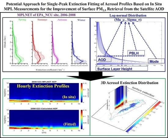
Potential Approach for Single-Peak Extinction Fitting of Aerosol Profiles Based on In Situ Measurements for the Improvement of Surface PM_2.5 Retrieval from Satellite AOD Product

Abstract

The vertical distribution of aerosols is important for accurate surface PM_2.5 retrieval and initial modeling forecasts of air pollution, but the observation of aerosol profiles on the regional scale is usually limited. Therefore, in this study, an approach to aerosol extinction profile fitting is proposed to improve surface PM_2.5 retrieval from satellite observations. Owing to the high similarity of the single-peak extinction profile in the distribution pattern, the log-normal distribution is explored for the fitting model based on a decadal dataset (3248 in total) from Micro Pulse LiDAR (MPL) measurements. The logarithmic mean, standard deviation, and the height of peak extinction near-surface (Mode) are manually derived as the references for model construction. Considering the seasonal impacts on the planetary boundary layer height (PBLH), Mode, and the height of the surface layer, the extinction profile is then constructed in terms of the planetary boundary layer height (PBLH) and the total column aerosol optical depth (AOD). A comparison between fitted profiles and in situ measurements showed a high level of consistency in terms of the correlation coefficient (0.8973) and root-mean-square error (0.0415). The satellite AOD is subsequently applied for three-dimensional aerosol extinction, and the good agreement of the extinction coefficient with the PM_2.5 within the surface layer indicates the good performance of the proposed fitting approach and the potential of satellite observations for providing accurate PM_2.5 data on a regional scale.

1. Introduction

As atmospheric aerosols significantly affect the climate and atmospheric environment [1,2,3,4], research in this area has attracted much attention across both academic disciplines and decision-making settings around the globe. Fine and surface level aerosol particles are known as particulate matter (PM). An increase in the PM_2.5 (i.e., PM with an aerodynamic diameter equal to or smaller than 2.5 μm) concentration not only impedes visibility but also threatens human health and causes premature mortality [5,6,7,8,9]. Ground-based monitoring networks are able to obtain precise PM_2.5 measurements, but are generally limited to sparse spatial resolution [10]. In recent decades, many studies have investigated the use of satellite-derived aerosol optical depth (AOD) for the estimation of surface PM_2.5 over a large spatial scale. AOD has been used to assess ground-based PM_2.5 mass since 2003 [11,12]. Since then, the relationship between satellite-derived AOD and surface PM_2.5 concentrations has been vigorously investigated in various regions of the world [13,14,15,16,17,18,19,20,21,22,23,24]. A good linear correlation between the AOD and PM has been found, despite the large accuracy differences among regions. The factors showing accuracy discrepancy, such as meteorological and aerosol properties, contribute to the AOD–PM relationship, namely, the vertical structure, composition, size distribution, and water content of atmospheric aerosols [16,25]. Several studies [26,27,28] have investigated those factors and revealed that the AOD–PM_2.5 relationship improves significantly when the vertical profile and relative humidity are taken into account. In addition, the effects of aerosol characteristics (e.g., the aerosol chemical composition or size distribution) have been examined [29]; the results showed that humidity correction (hygroscopic growth, particle mass extinction efficiency, and size distribution) and vertical correction improve AOD–PM_2.5 correlations.

LiDAR (light detection and ranging) stands out as an excellent tool for measuring aerosol vertical distributions. The network system Micro Pulse LiDAR network (MPLNET) was developed by NASA (National Aeronautics and Space Administration in U.S.) in 2000, and its application has shown its ability to determine the origin of aerosols by the aerosol layer height [30,31]. Since then, LiDAR-derived aerosol extinction profiles have significantly improved the correlation between AOD and surface PM_2.5 [27,32,33]. For instance, Wang et al. [27] used MPL data to analyze the extinction profiles of aerosols and classified them into near-surface, mixed, and two-layer transport types on a seasonal basis. They found that near-surface aerosol transport (0–2 km) is due to the long-range transport of aerosols and local pollutants that occur in the wintertime. Upper layer aerosol transport (2–4 km) is affected by the convective mixing/dispersion of aerosols from the Indochina Peninsula and Southeast China in the free atmosphere, which occurs during the springtime. The former carries aerosols originating from the burning of biomass, while the latter carries synthetic aerosols.

Regular parameterization schemes on the modeling of aerosol profiles often assume that aerosols within the planetary boundary layer (PBL) are homogeneously mixed to simplify the data analysis procedure. Nevertheless, this single-layer structure approach is not applicable in many real-life situations [16,34,35]. Consequently, Tsai et al. [16] illustrated a two-layer aerosol model characterized by well-mixed aerosol extinction in the PBL, and found that the aerosol extinction coefficient decreased exponentially with height above the top of the PBL from LiDAR observations. The estimations of the extinction coefficient at the surface in this model were found to be better than those in the single-layer model. The authors found a strong seasonality in the relationship between multiyear AERONET (i.e., AErosol RObotic NETwork) AOD and MPLNET extinction profile data. Furthermore, Chu et al. [17] extended their approach and concept to further explore the extinction profiles of aerosols of three classification types: aloft, well-mixed, and constrained. The extinction profiles had the largest aerosol abundance in the presence of aloft aerosols above the PBL, followed by well-mixed and constrained aerosols. The relative coefficients of the method were highly correlated in spring, autumn, and winter, with correction coefficients greater than 0.8.

In short, the aerosol profile (vertical distribution) provides crucial information for the retrieval of surface PM_2.5 in terms of columnar AODs. Although the aerosol profile can be provided from cloud-aerosol LiDAR and infrared pathfinder satellite observations (CALIPSO) of spaceborne and ground-based MPL, the point measurements are limited by their poor spatial coverage and infrequent observations. Therefore, the main objective of this study was to map the aerosol extinction profiles of columnar AODs at the regional scale. The log-normal distribution with high similarity to the single-peak aerosol extinction profile (according to the ground-based measurements) was examined as the fitting model for the regular representation of the vertical distribution of aerosols. The fitting model was further applied to the satellite AOD products after being validated by ground-based MPL observations. The results of the application suggest that the proposed approach can assist researchers in (1) building columnar AOD and planetary boundary layer height (PBLH) friendly aerosol extinction profiles, (2) expanding the level of satellite products in three-dimensional (3D) extinction, and (3) further improving the AOD–PM_2.5 relationships within the surface layer.

2. Materials and Methods

2.1. Data Sets

Four datasets were used in this study, namely, AERONET AOD, the MPLNET extinction profile, Middle Resolution Imaging Spectroradiometer (MODIS) AOD, and GEOS-5 FP (Goddard Earth Observing System, forward processing) PBLH; all were initiated and provided by NASA and are used to enhance NASA’s Earth Observations program and support NASA’s Earth Science mission. Ground-based measurements were taken from AERONET and MPLNET. The MPLNET dataset used in this study included the aerosol extinction profile, PBLH, and the observation times and dates. The AOD dataset was taken from the AERONET sun photometer. The satellite datasets applied were the MODIS AOD products and GMAO (Global Modeling and Assimilation Office) PBLH products for three-dimensional (3D) extinction over the regional scale.

2.1.1. In Situ Measurements

AERONET is a ground-based remote sensing aerosol network that was established by NASA and its partners [36]. The project aims to provide a long-term, continuous, and free-access aerosol database, and has been broadly used to validate aerosol retrieval from different satellite platforms. Direct sun measurements are performed using a sun photometer with a 1.2° full angle field of view every 15 min at wavelengths of 340, 380, 440, 500, 675, 870, 940, and 1020 nm [37]. In this study, the Level 2.0 cloud-screened and quality-assured AOD data at 500 nm (~0.01–0.02 uncertainty) were downloaded from the AERONET website for the period from January 2005 to December 2014 [38].

MPL Type 4 was manufactured by the Sigma Space Corporation (United States). The MPL is an eye-safe and compact LiDAR system that can be used to detect both aerosols and clouds at 527 nm. The recorded signals are stored with a 1-min time resolution and a 0.075-km vertical resolution. The principle of micropulsed light was described in detail by Campbell et al. and Welton et al. [39,40]. The extinction profile is theoretically associated with the AOD characteristic, which is defined as the integration of the extinction coefficient with the path throughout the atmosphere. The mathematical formula for the AOD is shown below:

$$\mathsf{\tau }\left(\mathsf{\lambda }\right)={{\displaystyle \int }}_0^{\mathrm{TOA}}{\mathsf{\alpha }}_{\mathrm{ext}}\left(\mathsf{\lambda },\mathrm{z}\right)\mathrm{dz}$$

(1)

where τ and ${\mathsf{\alpha }}_{\mathrm{ext}}$ are AOD and extinction profile, respectively, TOA is the top of the atmosphere, λ stands for wavelength, and z indicates the altitude.

In this research, the cloud-free aerosol extinction profiles and planetary boundary layer (PBL) data used were version 2 level 1.5a products (~0.27 km uncertainty) [41,42]. The time resolution for each product was selected to match the AERONET data on temporal grids (frequency of observation: 1 observation/20 min). The aerosol loading in the PBL is much higher than that in the free troposphere, as it is directly in contact with the Earth’s surface and responds to the surface within an hour or less [43]. Aerosol emissions at the surface of the Earth are mixed thoroughly in the PBL by turbulent motion and convection activity near the surface. Hence, the PBL provides valuable information about the conversion relationship between the log-normal distribution parameters. For this study, the PBLHs were less than 2.5 km, with the vast majority being less than 1.5 km. The average PBLH was 0.96 km in all cases. The average maximum Mode value was 0.45 km.

The MPL and sun photometer are both operated from the National Central University (NCU) campus at the same location (24.976° N, 121.185° E), named the MPLNET NCU_Taiwan site and the AERONET EPA-NCU site, where the elevation is 135 m above sea level. They have been used to collect aerosol extinction profiles and total column AOD data since 1999 and 1998, respectively. The site is located at the Chungli District of Taoyuan City in Taiwan, and is not exposed to significant local emission sources from nearby areas. The site location is in a subtropical climate zone with four distinct seasons: it is humid and cloudy in spring and summer and dry and relatively clear in fall and winter. The atmospheric environment in this region has been intensively influenced by the northeastern monsoons from the East China Sea and the southwestern monsoons from Southeast Asia, which prevail in winter and summer, respectively. These monsoons are associated with the long-range transport of air pollution from many regional pollutant sources to the Taiwan area [44].

2.1.2. MODIS AOD

MODIS is a spaceborne instrument that is mounted on the sun synchronous Terra and Aqua satellites. Terra has a morning overpass (local time), while Aqua has an afternoon overpass. The standard data products used in this study were downloaded from the National Aeronautics and Space Administration (NASA) Atmospheric Archive and Distribution System [45]. MODIS AOD data are retrieved using spectral radiance from the visible-near infrared (0.47–2.1 µm) wavelengths at a 10 km resolution at nadir. In this study, AOD data from MOD04 level-2 aerosol products at a 3 km spatial resolution (±0.05+20% uncertainty) were used as the input data for the aerosol extinction profiles, because the 3 km product has better resolution than the 10 km product for aerosol gradients, clouds, and shorelines [46].

2.1.3. GEOS-5 FP PBLH

The goal of the GMAO is to maximize the impact of satellite observations on the analyses and predictions of the Earth’s environment using computer algorithms and data assimilation techniques. The product required for this study was the GEOS-5 FP PBLH (planetary boundary layer height). The PBLH data field were used with an hourly 1/4 × 1/3 degree (0.25° lat. by 0.3125° lon.) spatial resolution (~0.27 km uncertainty). This is provided on the GMAO website, which was launched on December 1, 2007 [47].

2.2. Fitting Approach

2.2.1. Log-Normal Distribution

The log-normal distribution is a continuous probability distribution in which the logarithm of a random variable is normally distributed. The probability density function (pdf) for the log-normal distribution is derived as shown below:

$$f\left(\mathrm{x}|\mathsf{\mu },\mathsf{\sigma }\right)=\frac{1}{\mathrm{x}\mathsf{\sigma }\sqrt{2\mathsf{\pi }}}\exp \left\{\frac{-{\left(\mathrm{lnx}-\mathsf{\mu }\right)}^2}{2{\mathsf{\sigma }}^2}\right\}$$

(2)

where x is random variable, µ is the logarithmic normal mean with a range of $-\infty \le \mathsf{\mu }\le \infty$ and $\mathsf{\sigma }$ is the logarithmic normal standard deviation with a range of $\mathsf{\sigma } \ge 0$. In terms of the parameter characteristics, μ relates to the location of the peak value, and σ affects the width of the curve of the pdf.

The Mode is defined as the maximum point of the probability density function (i.e., a value at which the probability density function attains its maximum value). In particular, the Mode is the peak of the log-normal distribution. The mathematical expression of Mode is given by

$$\mathrm{Mode}={\mathrm{e}}^{\left({\mathsf{\mu }-\mathsf{\sigma }}^2\right)}$$

(3)

Log-normal distribution has most often been used to predict aerosol size distributions in previous studies [48,49,50,51]. As a result of its high similarity to the single-peak aerosol extinction profile, log-normal modes have also been used to represent the vertical distribution of aerosols in the literature [52,53]. Based on the LiDAR measurements at the NCU_Taiwan site, the seasonal extinction profile of aerosols exhibited a similar log-normal distribution after being rotated 90 degrees clockwise. Figure 1a demonstrates an example of the use of the log-normal distribution to fit an extinction profile. Regular practices have assumed that aerosols below the PBL are uniformly distributed. Aerosols below the PBL still have nonuniform distribution characteristics, as shown in Figure 1a,b. In the single-peak aerosol extinction profiles, there is an aerosol layer with a relatively large extinction coefficient below the PBL. The information in this layer has a significant impact on the subsequent conversion of the log-normal distribution parameters. This notion will be discussed further in the following section. The aerosol vertical distributions on 9 May 2009 are illustrated in Figure 1a, together with the distributions retrieved by the sun photometer for comparison. Both distributions appear slightly different below a height of 10 km. This difference may be caused by the presence of a small amount of aerosol above 10 km.

In this study, the aerosol extinction profiles were assumed to preserve the characteristics of a log-normal distribution. Additionally, the vertical and horizontal axes of the log-normal distribution were converted to the aerosol extinction coefficient and height, respectively. Due to the pattern of the extinction profile being apparently affected by the levels of PBLH (Figure 1b) and columnar AOD, the log-normal distribution variables (logarithmic mean, standard deviation, and Mode) were proposed to determine the PBLH and columnar AOD (see Figure 1c).

2.2.2. Fitting Procedure for the Single-Peak Extinction Profile

A decadal MPLNET and AERONET dataset was collected from January 2005 to December 2014. To ensure the data quality was sufficient, the following criteria were used: (1) only data collected at 08:00–18:00 local time were examined (night time data were excluded due to not available data); (2) AERONET data with a 20-min interval were matched with the MPLNET observations; (3) the aerosols from long-range transport, which generally present in higher layers and result in a bimodal or multiple peaks of the aerosol profile, were excluded; and (4) profiles of PBLH above 2.5 km were also excluded. Eventually, out of 6118 extinction profiles, a total of 3248 pairs of MPLNET extinction profiles and AERONET columnar AODs were selected to construct the fitting approach. According to the limitations of the MPL observations, the extinction coefficients below 0.2 km were excluded in the fitting procedure. Instead, the well-mixed layer was induced as the surface layer.

The probability density function (pdf) of MATLAB (matrix laboratory) software package was employed to examine the best fitting parameters for each aerosol extinction profile. The total AOD was used as a constraint on a randomly chosen set of initial values. The Mode (i.e., the height of the maximum value of the extinction profile) was chosen according to the characteristics of the single-peak aerosol extinction profiles to represent the maximum height of the extinction coefficient. In addition, the conversion relationship for each variable was elucidated. The regression analysis and conversion equation procedures used in this study are illustrated in Figure 2.

Regression analysis was applied to evaluate the relationship between ground-based meteorological data (PBLH and AOD) and logarithmic normal parameters (i.e., the logarithmic normal mean μ and the logarithmic normal standard deviation σ). The aerosol extinction profiles were mapped by the log-normal distribution. The integrated area under the log-normal distribution (equal to one) was multiplied by a fitting variable (scaling) as the adjustment. Accordingly, the fitting function f(x) was determined by the following equation,

$$\mathrm{f}\left(\mathrm{x}\right)=\mathrm{Area}\times \mathrm{logarithmic} \mathrm{normal}\left(\mathsf{\mu },\mathsf{\sigma }\right)$$

(4)

where Area is the integral under the extinction profile, which is equivalent to the AOD. The fitting curve shape was then determined by the two logarithmic normal parameters (μ and σ), which were derived from the AOD, the PBLH, and the surface extinction coefficient (0.2 km) via the profile fitting process.

The log-normal distribution approached zero at the original point, which conflicts with the real situation of the aerosol extinction profile. Therefore, the height of the well-mixed layer was determined to modify the fitting profile near the surface. Based on the near-surface extinction of the ground truth data, we adjusted the height of the well-mixed layer along with the change in the Mode in order to retrieve a better fitting result.

3. Results and Analyses

In this study, the log-normal distribution was used to map aerosol profiles within the boundary layer near the surface. Fitted log-normal variables were obtained based on the in situ dataset observed from only one AERONET and MPLNET site in Taiwan. A further regression analysis was conducted to explore the conversion relationships among the fitted log-normal variables, columnar aerosol optical depth, and planetary boundary layer height. A single-peak aerosol extinction profile was established through the integration of ground truth, meteorological, and satellite remote sensing data. In this manner, the aerosol profiles in the area with no AERONET or MPLNET sites but with satellite AOD and PBLH information could be estimated and retrieved. Furthermore, independent analyses on seasonality impacts were carried out. Additionally, a comparison between the MODIS AOD and GMAO products using surface extinction coefficient inversion and the two-dimensional aerosol profile was conducted. The fitting results of a decadal dataset show that this approach is able to determine the three-dimensional aerosol extinction distribution and is applicable to satellite observations of surface PM concentrations.

3.1. Impacts of AOD and PBLH on the Extinction Profile

To fit the aerosol extinction profiles in this study, AOD and PBL were used as essential information to obtain the log-normal distribution parameters. Therefore, the relationships among the AOD, PBL, and surface extinction coefficient (0.2 km) were explored to assess the feasibility of the proposed method for subsequent analysis. Figure 3a shows the scatter plot for the surface aerosol extinction coefficient and AOD corresponding to the PBL height (PBLH). The results show that the corresponding surface aerosol extinction coefficient is greater than that determined using the same AOD values but a lower PBLH. These results are consistent with a previous study [54], which stated that aerosols are concentrated on the surface during dusty or hazy events, and the development of the PBL is hindered, resulting in a lower height. Therefore, it can be inferred that the PBLH and AOD influence the surface extinction coefficient. For further clarification, the surface aerosol extinction coefficient and AOD corresponding to the Mode are illustrated in Figure 3b. The result indicates that the distribution of the Mode is more regular than that of the PBLH. For a given AOD level, a larger Mode corresponds to smaller extinction coefficients, and vice versa. Therefore, we infer that the Mode has a relationship with the surface extinction coefficient and is a very important parameter. As shown in Figure 3a,b, the distribution patterns of the PBLH and Mode versus the surface extinction appear to be similar. The Mode pattern is more distinct and much clearer than that of the PBLH. The PBLH and the Mode both have impacts on the aerosol vertical distribution.

3.2. Log-Normal Distribution in Terms of the AOD and PBLH

As mentioned previously, the PBLH and Mode are both related to the vertical distribution of aerosols. For further elaboration, a regression analysis and comparative analysis were conducted to explore their characteristics. As shown in Figure 4, the logarithmic normal standard deviation (σ) increases as the PBLH and Mode increase. The Mode decreases, the PBLH increases, and the logarithm standard deviation (σ) becomes larger, and vice versa.

The relationship between the PBLH and the Mode has the potential to determine the aerosol extinction profiles and the corresponding characteristics. We defined two parameters to represent the quantitative relationship between the PBLH and the Mode, namely, $\mathsf{\Delta }\mathrm{h}$ and the $\mathrm{Height} \mathrm{Ratio}$; the procedure can be expressed as follows:

$$\mathsf{\Delta }\mathrm{h}=\mathrm{PBLH}-\mathrm{Mode}$$

(5)

$$\mathrm{Height} \mathrm{Ratio}=\frac{\mathrm{PBLH}}{\mathrm{Mode}}$$

(6)

where $\mathsf{\Delta }\mathrm{h}$(km) is the relative height difference, and $\mathrm{Height} \mathrm{Ratio}$(-) is the relative height ratio. $\mathsf{\Delta }\mathrm{h}$(km) and Height Ratio(-) are used for the subsequent analysis and discussion throughout this paper. These two parameters are complementary to each other, and are able to determine the category of aerosol extinction profiles; therefore, they can be used to obtain the log-normal distribution parameters. The MODIS AOD and GMAO PBLH are the datasets used to obtain the log-normal distribution parameters. The Mode can be derived from the relationship between the PBLH and AOD. To discover the possible linear relationships among these parameters, we used the scatter plot of $\mathsf{\Delta }\mathrm{h}$ versus the PBLH and AOD to determine whether good correlations existed, as shown in Figure 5. For further analysis, we divided the AOD into several categories and conducted a multiple regression analysis. The resulting linear relationships between Δh and the PBLH are shown in

Table 1. The linear relationships between Δh and the PBLH for various AOD (aerosol optical depth) levels.

AOD	Slope	Offset	R	RMSE	Data Point	Mean AOD	P-Value a
0.00–0.05	1.037	0.3154	0.9984	0.1044	84	0.025	<0.001
0.05–0.10	1.191	0.2303	0.9935	0.0334	286	0.075	<0.001
0.10–0.15	1.110	0.2954	0.8217	0.1344	561	0.125	<0.001
0.15–0.20	1.163	0.2762	0.9951	0.0232	594	0.175	<0.001
0.20–0.25	1.163	0.3081	0.6815	0.1527	498	0.225	<0.001
0.25–0.30	1.038	0.4288	0.9967	0.0246	343	0.275	<0.001
0.30–0.35	1.279	0.3291	0.9908	0.0283	225	0.325	<0.001
0.35–0.40	1.300	0.3376	0.9924	0.0361	180	0.375	<0.001
0.40–0.45	1.139	0.4237	0.9796	0.0435	156	0.425	<0.001
0.45–0.50	1.219	0.4372	0.9722	0.0452	136	0.475	<0.001
0.50–0.55	1.137	0.4403	0.9736	0.0394	115	0.525	<0.001
0.55–0.60	1.182	0.4554	0.9641	0.0531	70	0.575	<0.001

^a General linear regression was used to test for.

.

By integrating Figure 5 and Table 1, the following general Mode conversion equation was obtained:

$$\mathrm{PBLH}=\mathrm{S}\times \left(\mathrm{A}\times \mathsf{\Delta }\mathrm{h}+\mathrm{f}\left(\mathrm{AOD}\right)\right)$$

(7)

where S (=3.37) is the Scale adjustment for seasonal variation (see also Section 3.3), A is the slope of the relative height difference (Δh), and f (AOD) is a function of AOD and is the offset (intercept) of the regression results shown in Table 1. Since AOD has little influence on the slope, S was used to adjust the slope for seasonal variation. f (AOD) was then obtained from Table 1 and was derived as

$$\mathrm{f}\left(\mathrm{AOD}\right)=\mathrm{offset}=0.36\times \mathrm{AOD}+0.2484$$

(8)

Then, the value of the Mode (CMode) could be calculated from Equation (9),

$$\mathrm{CMode}=\left(\frac{0.2\times \mathrm{PBLH}+0.1\times \mathrm{AOD}-0.065}{1.163}\right)\times \mathrm{S}$$

(9)

The empirical CMode identification in Equation (9) shows the feasibility of deriving the Mode from the PBLH and AOD, which are metrological datasets. Based on the CMode values calculated from Equation (9), for profiles over 1.5 km PBLH, the discrepancy between the calculated CMode and the fitted Mode was significant, but only for a few cases. Therefore, these rare cases are considered to be highly uncertain and were excluded from the further analysis, i.e., the height range of cases lower than 1.5 km and greater than 0.2 km (compliant with the minimum height detectability of the MPL instruments) were included. The regression analysis conducted after screening showed that the calculated CMode and fitted Mode appeared to have good agreement, as shown in Figure 6. The correlation coefficient (R) and RMSE values were 0.8014 and 16.1%, respectively.

The regression analysis of the AOD, PBLH, and Mode was applied to obtain the log-normal distribution parameters (i.e., the mean and standard deviation). Equation (3) shows that both the log mean (μ) and log-normal standard deviation (σ) have a conversion relationship with the Mode (which indicates the height of the maximum extinction coefficient). Accordingly, each Mode in the normal distribution has its corresponding logarithmic normal parameters. In this study, σ was taken as the major parameter due to its ability to determine the aerosol layer height. In addition, the Mode, PBLH, relative height difference (Δh), and relative height ratio (Height Ratio) were integrated into the analysis of the conversion relationship with σ. After summarizing the data characteristics and performing various tests, we deduced a combined parameter to analyze the conversion relationship of σ. This combined parameter is denoted by CSigma, which is defined as

$$\mathrm{CSigma}=\mathsf{\sigma }\times \mathsf{\Delta }\mathrm{h}\times \left(\mathrm{PBLH}-\mathrm{Scale}\times \mathrm{Mode}\right)$$

(10)

where Scale is an adjustment variable and is dimensionless. The scale was selected when dealing with different values of σ. According to the characteristics of the cases in this study, different values of Scale adjustment (S) for seasonal variation are necessary to match the data distribution of low Δh and high Δh, respectively. The method used to derive CSigma was similar to the CMode conversion formula. A regression analysis was carried out to analyze the effect of Δh in different intervals. The relative relationships among the parameters were eventually sorted out. The regression results are shown in

Table 2. The linear regression analysis of the relative height difference (Δh) of different segments with a Scale of 1.3.

Δh	Slope	Offset	R	P-Value a
0.00–0.20	17.115	1.3	0.756	<0.001
0.20–0.25	13.863	1.3	0.840	<0.001
0.25–0.30	11.251	1.3	0.792	<0.001
0.30–0.35	9.7043	1.3	0.750	<0.001
0.35–0.40	8.6445	1.3	0.684	<0.001

^a General linear regression was used to test for.

and

Table 3. The linear regression analysis of the relative height difference (Δh) of different segments with a Scale of 2.5.

AOD	Slope	Offset	R	P-Value a
0.30–0.35	8.277	2.5	0.2014	<0.001
0.35–0.40	7.124	2.5	0.7593	<0.001
0.40–0.45	6.148	2.5	0.8747	<0.001
0.45–0.50	5.584	2.5	0.9064	<0.001
0.50–0.55	5.486	2.5	0.9167	<0.001
0.55–0.60	5.412	2.5	0.8908	<0.001
0.60–0.65	4.336	2.5	0.933	<0.001
0.65–0.70	4.129	2.5	0.9205	<0.001
0.70–0.75	3.687	2.5	0.9673	<0.001
0.75–0.80	3.590	2.5	0.9533	<0.001
0.80–0.85	3.180	2.5	0.9818	<0.001
0.85–0.90	2.954	2.5	0.9910	<0.001
0.90–0.95	3.191	2.5	0.9671	<0.001
>0.95	3.425	2.5	0.6446	<0.001

^a General linear regression was used to test for.

for Scales 1.3 and 2.5, respectively. For the CSigma calculation in Equation (10) based on the regression results, a Scale of 1.3 was adopted to calculate dataset cases where Δh < 0.35 km, and a Scale of 2.5 was adopted for dataset cases where Δh ≥ 0.35 km.

Below, the procedure for the conversion of σ is elaborated. The piecewise linear regression equation, which can be derived from Table 2 and Table 3, is as follows:

$$\mathrm{Height} \mathrm{ratio}=\mathrm{Slope}\times \mathsf{\sigma }\times \mathsf{\Delta }\mathrm{h}\times \left(\mathrm{PBLH}-\mathrm{Scale}\times \mathrm{Mode}\right)+\mathrm{Scale}$$

(11)

$$=\mathrm{Slope}\left(1.3/2.5\right)\times \mathrm{CSigma}+\mathrm{Scale}$$

Slope (1.3) = –32.13 × Δh + 20.47

(12)

Slope (2.5) = –7.309 × Δh + 9.255

(13)

Finally, the calculated log-normal standard deviation (CSigma) equations were obtained by substituting Equations (12) and (13) into Equation (11). The resulting log-normal standard deviation conversion formulas can be expressed as

$${\mathrm{CSigma}}_{\mathrm{Slope} \left(1.3\right)}=\frac{Height ratio-1.3}{\left(-32.13\times \mathsf{\Delta }\mathrm{h}+20.47\right)\times \mathsf{\Delta }\mathrm{h}\times \left(PBLH-1.3\times Mode\right)}$$

(14)

$${\mathrm{CSigma}}_{\mathrm{Slope} \left(2.5\right)}=\frac{Height ratio-2.5}{\left(-7.309\times \mathsf{\Delta }\mathrm{h}+8.81\right)\times \mathsf{\Delta }\mathrm{h}\times \left(PBLH-2.5\times Mode\right)}$$

(15)

Verification of Equations (14) and (15) was conducted using dataset cases where Δh < 0.35 km and Δh ≥ 0.35 km. The resulting RMSE values were 25.3% and 16.47%, respectively. The fitting results are illustrated in Figure 7a,b, respectively.

3.3. Scale Adjustment for Seasonal Variation (S)

To investigate the Mode conversion relationship in different seasons, the S-parameter (S = 3.37) defined in Equation (7) was determined by optimizing the seasonal variation. There were more dataset cases in autumn and winter than in spring and summer. A possible reason for this is that the weather conditions in autumn and winter are dry and stable under high-pressure systems, which leads to more effective observations than in spring and summer. The optimized S-parameters for all seasons indicate that the value for the spring season, i.e., S = 3.34, is smaller than the typical value of S = 3.37, and the S-parameters of the other three seasons all have greater values than the typical value, with the highest value in autumn (3.49), followed by winter (3.47) and summer (3.43). In addition, the original mean error of the Mode conversion relationship described in Equation (9) was found to be 16.1% without consideration of the seasonal variation. After seasonal analysis and S-parameter optimization, the mean error of the summer season was shown to be the smallest among all seasons (i.e., spring: 14.65%; summer: 11.77%; autumn: 13.53%; and winter: 14.22%). The mean errors for the calculated log-normal standard deviation (σ) described in Equations (14) and (15) at Scales of 1.3 and 2.5 were 25.3% and 16.47%, respectively. The differences in standard deviation (σ) were not significant in the different seasons after seasonal analysis and adjustment, which indicates that the conversion relationship remains valid for all seasons.

3.4. Identifying the Height of the Surface Layer

The fitting of a log-normal distribution theoretically approaches zero at the original point (i.e., at the surface exactly), which is an issue for aerosol profiles. Due to the limitation of ground-based MPL, a height of 0.2 km above the surface is generally set for the thickness of the surface layer. The fixed setting of the surface layer height may induce uncertainty in fitting the extinction profile, as shown in Figure 8a. The results of the calculated near-surface (approximately 0.2 km) extinction show that the correlation decreased as the Mode increased, indicating the effect of the surface layer height variable. To address the fitting uncertainty for extinction on the surface layer, the height of the surface layer needed to be determined. Under the assumption of a well-mixed layer, the height of the surface layer was determined along with the Mode corresponding to the lowest RMSE compared with the ground-truth data. Figure 9a,b illustrates the determination of the surface layer height in different intervals of the Mode for the dataset cases where Δh < 0.35 km and Δh ≥ 0.35 km, respectively. The results of the regression analysis and the mean Mode height used in this study indicate that mean extinction coefficients below 500 m are consistent with those present in in situ situations. The correlation between the calculated extinction coefficient and the observed MPLNET extinction coefficient after adjusting the near-surface well-mixed layer indicated a greater level of agreement, as shown in Figure 8b. The correlation coefficient (R) and the RMSE were 0.8973 and 0.0415 (p-value < 0.001), respectively.

3.5. Validation and Application of a Case Study

To explore and demonstrate the applicability of the proposed log-normal fitting method, the case studies of the extinction profile fitted with columnar AOD from EPA-NCU AERONET during the daytime associated with GEOS-5 FP PBLH were examined; three sets of fitted results are shown in Figure 10. The temporal results of the fitted extinction profiles were in good agreement with the in situ measurements of the MPLNET NCU_Taiwan site, indicating the practicality of the fitting approach.

The application of the fitting approach to satellite observations in the extinction profile was explored. Mode conversion (CMode) in Equation (9) and log-normal σ conversion (CSigma) in Equation (14) were integrated into the Aqua and Terra MODIS AOD products (Figure 11a) and GMAO GEOS-5 FP products (Figure 11b) in Taiwan for October 29, 2014 (indicated using local time (LT)). The application procedure involved the following steps: First, to deal with the spatial and temporal variability in the products, PBLH products were interpolated to a 3 km spatial resolution to match the MODIS AOD products. Then, we determined the MPLNET station position and compared the PBLH products, and the GEOS-5 FP PBLH product was calibrated using its ratio with the ground-truth dataset (MPLNET) (Figure 11c). According to the models proposed herein, three input parameters are required to carry out the log-normal distribution variable conversion, namely, the AOD, PBLH, and Mode (aerosol layer height). The Mode conversion was performed using Equation (9), and the seasonal adjustment S-parameter was selected as S = 3.43. Second, the calculated σ was obtained by using Equations (14) and (15), which were presented in the previous section. Finally, the logarithmic σ obtained with the Mode was used to retrieve the logarithmic mean (μ). The results of the logarithmic σ and logarithmic μ are displayed in Figure 11d,e, respectively. For the extinction coefficient of surface layer, we first determined the height of surface layer based on the results illustrated in Figure 9 under the assumption that aerosols below 500 m were in a well-mixed state. The surface extinction coefficient was further calculated along with the fitted extinction profile within surface layer height, as shown in Figure 11f.

To further understand the correlation between the PM_2.5 concentration and the MODIS AOD, PM_2.5 data were collected from the EPA-NCU station on October 29, 2014 at 12:55 LT (18 data points). Although both of the extinction profiles fitted with the PBLH from GEOS-5 FP PBLH (Figure 12a) and MPLNET PBLH (Figure 12b) were acceptable, it was recommended that accurate PBLH information be used due to the better results from fitting with the MPLNET PBLH (Figure 12b). The 3D distribution of aerosol extinction was then constructed using columnar AOD from the MODIS product over the region of Taiwan, as displayed in Figure 13a. The corresponding scatter plots of the surface extinction coefficient and the ground-based PM_2.5 data (Figure 13b) depicted in Figure 13c were eventually compared. The strong correlations between extinction and PM_2.5, i.e., R =0.7459 (p-value < 0.001) indicate the higher accuracy of the proposed log-normal fitting approach, which demonstrates its potential application for particulate matter estimation via satellite remote sensing, which is associated with accurate PBLH information in Taiwan.

4. Discussion

The single-peak aerosol extinction profiles were examined with a decadal MPL dataset. Based on the characteristics of the log-normal distribution, the height of the maximum extinction coefficient (Mode) in the single-peak extinction profile was found to play a significant role in the adjustment of the surface layer thickness and seasonal variation, as per the issues pointed out by the previous studies [16,17,35]. Therefore, a Scale adjustment that is dependent on the Mode was proposed to address height ambiguity issues (i.e., the seasonal change in the PBLH–Mode height difference) and to determine the height of the surface layer (well-mixed). The accuracy of fitted extinction profiles was significantly ameliorated after the Scale adjustment and surface layer height determination (also see the results shown in Figure 8b).

Further application of satellite data to 3D aerosol extinction (Figure 13a) yielded promising results related to the estimation of surface PM_2.5 (Figure 13b) in Taiwan. The case study indicated that satellite data should be used in conjunction with accurate PBLH information. The PBLH needs to be estimated correctly in order to comply with the real situation, specifically for areas in mountains or in cases of higher PBLH values [34]. The PBLH appears to have a greater influence on the derived distribution of extinction coefficients. Generally, an excessively high PBLH leads to underestimations of the surface extinction coefficients.

5. Conclusions

Concerning the uncertainty associated with assuming well-mixed aerosols within the planetary boundary layer, a sensible aerosol vertical distribution described by a log-normal function is proposed in this study to give more realistic extinction profile fitting. The accuracy of single-peak fitting of aerosol extinction profiles was improved by considering the seasonal variation between the PBLH and the Mode and the variable surface layer height. The proposed fitting approach, which is based on PBLH and columnar AOD information, further offers a potential solution for establishing a three-dimensional (3D) aerosol extinction profile. The consistent results of the case study between surface extinction and PM_2.5 suggests the practicality of satellite observations for providing reasonable surface PM_2.5 data on a regional scale, which facilitates the application of remote sensing in air quality monitoring.

Nevertheless, future efforts are required to complete the aerosol extinction profile fitting approach to address the following points: (1) due to the fact that the dataset was from a single stationed instrument only, this study is not representative of other situations. Data from multiple MPL sites should be collected in the future to obtain in situ extinction profiles, including data on seasonal variation, to extend the practicality of the fitting approach. (2) The log-normal distribution mapping approach applied here is limited to the single-peak (unimodal) aerosol profiles. For the application of long-range aerosol transportation, the mapping of aerosol profiles by the summation of log-normal modes is required, because aerosols transported over a long range produce higher levels of aerosol and result in bimodal or multimodal profiles in the aerosol profile. (3) A major goal of aerosol mapping is to retrieve the PM near the surface. Accurate PM estimation requires not only the aerosol extinction coefficient, but also the aerosol type and relative humidity of the aerosol particles to be known. It is thus expected that the relative humidity parameter will be integrated into the proposed log-normal fitting method to produce more robust results in the future.

References

1. Akimoto, H. Global air quality and pollution. Science 2003, 302, 1716–1719. [Google Scholar] [CrossRef] [Green Version]
2. Pöschl, U. Atmospheric aerosols: Composition, transformation, climate and health effects. Angew. Chem Int. Ed. 2005, 44, 7520–7540. [Google Scholar] [CrossRef] [PubMed]
3. Stocker, T.F.; Qin, D.; Plattner, G.-K.; Tignor, M.; Allen, S.K.; Boschung, J.; Nauels, A.; Xia, Y.; Bex, V.; Midgley, P.M. Climate Change 2013: The Physical Science Basis. Contribution of Working Group I to the Fifth Assessment Report of the Intergovernmental Panel on Climate Change; Cambrige University Press: New York, NY, USA, 2013. [Google Scholar] [CrossRef]
4. Wu, G.; Li, Z.; Fu, C.; Zhang, X.; Zhang, R.; Zhang, R.; Zhou, D. Advances in studying interactions between aerosols and monsoon in China. Sci. China Earth Sci. 2016, 59, 1–16. [Google Scholar] [CrossRef]
5. Caiazzo, F.; Ashok, A.; Waitz, I.A.; Yim, S.H.; Barrett, S.R. Air pollution and early deaths in the United States. Part I: Quantifying the impact of major sectors in 2005. Atmos. Environ. 2013, 79, 198–208. [Google Scholar] [CrossRef]
6. Li, C.; Mao, J.; Lau, A.K.; Yuan, Z.; Wang, M.; Liu, X. Application of MODIS satellite products to the air pollution research in Beijing. Sci. China Ser. D Earth Sci. 2005, 48, 209–219. [Google Scholar] [CrossRef]
7. Sacks, J.D.; Stanek, L.W.; Luben, T.J.; Johns, D.O.; Buckley, B.J.; Brown, J.S.; Ross, M. Particulate matter–induced health effects: Who is susceptible? Environ. Health Perspect. 2011, 119, 446. [Google Scholar] [CrossRef]
8. Owili, P.O.; Lien, W.-H.; Muga, M.A.; Lin, T.-H. The associations between types of ambient PM2.5 and under-five and maternal mortality in Africa. Int. J. Environ. Res. Public Health 2017, 14, 359. [Google Scholar] [CrossRef] [PubMed] [Green Version]
9. Lien, W.-H.; Owili, P.O.; Muga, M.A.; Lin, T.-H. Ambient particulate matter exposure and under-five and maternal deaths in Asia. Int. J. Environ. Res. Public Health 2019, 16, 3855. [Google Scholar] [CrossRef] [Green Version]
10. Zhang, G.; Rui, X.; Fan, Y. Critical review of methods to estimate PM2. 5 concentrations within specified research region. ISPRS Int. J. Geo Inf. 2018, 7, 368. [Google Scholar] [CrossRef] [Green Version]
11. Chu, D.A.; Kaufman, Y.; Zibordi, G.; Chern, J.; Mao, J.; Li, C.; Holben, B. Global monitoring of air pollution over land from the Earth Observing System-Terra Moderate Resolution Imaging Spectroradiometer (MODIS). J. Geophys. Res. Atmos. 2003, 108, 4661. [Google Scholar] [CrossRef]
12. Wang, J.; Christopher, S.A. Intercomparison between satellite-derived aerosol optical thickness and PM2.5 mass: Implications for air quality studies. Geophys. Res. Lett. 2003, 30, 2095. [Google Scholar] [CrossRef]
13. Engel-Cox, J.A.; Hoff, R.M.; Rogers, R.; Dimmick, F.; Rush, A.C.; Szykman, J.J.; Al-Saadi, J.; Chu, D.A.; Zell, E.R. Integrating lidar and satellite optical depth with ambient monitoring for 3-dimensional particulate characterization. Atmos. Environ. 2006, 40, 8056–8067. [Google Scholar] [CrossRef]
14. Koelemeijer, R.; Homan, C.; Matthijsen, J. Comparison of spatial and temporal variations of aerosol optical thickness and particulate matter over Europe. Atmos. Environ. 2006, 40, 5304–5315. [Google Scholar] [CrossRef]
15. Di Nicolantonio, W.; Cacciari, A.; Tomasi, C. Particulate matter at surface: Northern Italy monitoring based on satellite remote sensing, meteorological fields, and in-situ samplings. IEEE J. Sel. Top. Appl. Earth Obs. Remote Sens. 2009, 2, 284–292. [Google Scholar] [CrossRef]
16. Tsai, T.-C.; Jeng, Y.-J.; Chu, D.A.; Chen, J.-P.; Chang, S.-C. Analysis of the relationship between MODIS aerosol optical depth and particulate matter from 2006 to 2008. Atmos. Environ. 2011, 45, 4777–4788. [Google Scholar] [CrossRef]
17. Chu, D.A.; Tsai, T.-C.; Chen, J.-P.; Chang, S.-C.; Jeng, Y.-J.; Chiang, W.-L.; Lin, N.-H. Interpreting aerosol lidar profiles to better estimate surface PM2. 5 for columnar AOD measurements. Atmos. Environ. 2013, 79, 172–187. [Google Scholar] [CrossRef]
18. Yap, X.; Hashim, M. A robust calibration approach for PM10 prediction from MODIS aerosol optical depth. Atmos. Chem. Phys. Dis. 2013, 13, 3517–3526. [Google Scholar] [CrossRef] [Green Version]
19. Bilal, M.; Nichol, J.E.; Spak, S.N. A new approach for estimation of fine particulate concentrations using satellite aerosol optical depth and binning of meteorological variables. Aerosol Air Qual. Res. 2017, 11, 356–367. [Google Scholar] [CrossRef] [Green Version]
20. Stafoggia, M.; Bellander, T.; Bucci, S.; Davoli, M.; de Hoogh, K.; De’Donato, F.; Gariazzo, C.; Lyapustin, A.; Michelozzi, P.; Renzi, M.; et al. Estimation of daily PM10 and PM2.5 concentrations in Italy, 2013–2015, using a spatiotemporal land-use random-forest model. Environ. Int. 2019, 124, 170–179. [Google Scholar] [CrossRef]
21. Xue, T.; Zheng, Y.; Tong, D.; Zheng, B.; Li, X.; Zhu, T.; Zhang, Q. Spatiotemporal continuous estimates of PM2. 5 concentrations in China, 2000–2016: A machine learning method with inputs from satellites, chemical transport model, and ground observations. Environ. Int. 2019, 123, 345–357. [Google Scholar] [CrossRef]
22. Chelani, A.B. Estimating PM2. 5 concentration from satellite derived aerosol optical depth and meteorological variables using a combination model. Atmos. Pollut. Res. 2019, 10, 847–857. [Google Scholar] [CrossRef]
23. Zeydan, Ö.; Wang, Y. Using MODIS derived aerosol optical depth to estimate ground-level PM2. 5 concentrations over Turkey. Atmos. Pollut. Res. 2019, 10, 1565–1576. [Google Scholar] [CrossRef]
24. Lee, H.J. Benefits of high resolution PM2. 5 prediction using satellite MAIAC AOD and land use regression for exposure assessment: California examples. Environ. Sci. Technol. 2019, 53, 12774–12783. [Google Scholar] [CrossRef] [PubMed]
25. Van Donkelaar, A.; Martin, R.V.; Brauer, M.; Kahn, R.; Levy, R.; Verduzco, C.; Villeneuve, P.J. Global estimates of ambient fine particulate matter concentrations from satellite-based aerosol optical depth: Development and application. Environ. Health Perspect. 2010, 118, 847. [Google Scholar] [CrossRef] [PubMed] [Green Version]
26. Li, J.; Carlson, B.E.; Lacis, A.A. How well do satellite AOD observations represent the spatial and temporal variability of PM2.5 concentration for the United States? Atmos. Environ. 2015, 102, 260–273. [Google Scholar] [CrossRef]
27. Wang, Z.; Chen, L.; Tao, J.; Zhang, Y.; Su, L. Satellite-based estimation of regional particulate matter (PM) in Beijing using vertical-and-RH correcting method. Remote Sens. Environ. 2010, 114, 50–63. [Google Scholar] [CrossRef]
28. Zheng, S.; Pozzer, A.; Cao, C.; Lelieveld, J. Long-term (2001–2012) concentrations of fine particulate matter (PM 2.5) and the impact on human health in Beijing. China. Atmos. Chem. Phys. 2015, 15, 5715–5725. [Google Scholar] [CrossRef] [Green Version]
29. Lin, C.; Li, Y.; Yuan, Z.; Lau, A.K.; Li, C.; Fung, J.C. Using satellite remote sensing data to estimate the high-resolution distribution of ground-level PM2.5. Remote Sens. Environ. 2015, 156, 117–128. [Google Scholar] [CrossRef]
30. Welton, E.J.; Campbell, J.R.; Spinhirne, J.D.; Scott, V.S. Global monitoring of clouds and aerosols using a network of micropulse lidar systems. In Proceedings of the Lidar Remote Sensing for Industry and Environment Monitoring, Sendai, Japan, 9–12 October 2000. [Google Scholar]
31. Welton, E.J.; Stewart, S.A.; Lewis, J.R.; Belcher, L.R.; Campbell, J.R.; Lolli, S. Status of the NASA Micro Pulse Lidar Network (MPLNET): Overview of the network and future plans, new version 3 data products, and the polarized MPL. EPJ Web Conf. 2018, 176, 09003. [Google Scholar] [CrossRef] [Green Version]
32. Engel-Cox, J.A.; Holloman, C.H.; Coutant, B.W.; Hoff, R.M. Qualitative and quantitative evaluation of MODIS satellite sensor data for regional and urban scale air quality. Atmos. Environ. 2004, 38, 2495–2509. [Google Scholar] [CrossRef]
33. He, Q.; Li, C.; Mao, J.; Lau, A.K.H.; Chu, D. Analysis of aerosol vertical distribution and variability in Hong Kong. J. Geophys. Res. Atmos. 2008, 13, D14211. [Google Scholar] [CrossRef]
34. Chen, Y.; Zhao, C.; Zhang, Q.; Deng, Z.; Huang, M.; Ma, X. Aircraft study of mountain chimney effect of Beijing, china. J. Geophys. Res. Atmos. 2009, 114, D08306. [Google Scholar] [CrossRef]
35. Yongxiang, H.; Xiaomin, F.; Tianliang, Z.; Shichang, K. Long range trans-Pacific transport and deposition of Asian dust aerosols. J. Environ. Sci. 2008, 20, 424–428. [Google Scholar] [CrossRef]
36. Holben, B.N.; Eck, T.F.; Slutsker, I.; Tanre, D.; Buis, J.; Setzer, A.; Vermote, E.; Reagan, J.; Kaufman, Y.; Nakajima, T.; et al. AERONET—A federated instrument network and data archive for aerosol characterization. Remote Sens. Environ. 1998, 66, 1–16. [Google Scholar] [CrossRef]
37. Holben, B.; Tanre, D.; Smirnov, A.; Eck, T.; Slutsker, I.; Abuhassan, N.; Newcomb, W.W.; Schafer, J.S.; Chatenet, B.; Lavenu, F.; et al. An emerging ground-based aerosol climatology: Aerosol optical depth from AERONET. J. Geophys. Res. Atmos. 2001, 106, 12067–12097. [Google Scholar] [CrossRef]
38. AERONET (AErosol RObotic NETwork). Available online: https://aeronet.gsfc.nasa.gov/ (accessed on 1 September 2016).
39. Campbell, J.R.; Hlavka, D.L.; Welton, E.J.; Flynn, C.J.; Turner, D.D.; Spinhirne, J.D.; Scott, V.S.; Hwang, I.H. Full-time, eye-safe cloud and aerosol lidar observation at atmospheric radiation measurement program sites: Instruments and data processing. J. Atmos. Ocean. Technol. 2002, 19, 431–442. [Google Scholar] [CrossRef]
40. Welton, E.J.; Voss, K.J.; Quinn, P.K.; Flatau, P.J.; Markowicz, K.; Campbell, J.R.; Spinhirne, J.D.; Gordon, H.R.; Johnson, J.E. Measurements of aerosol vertical profiles and optical properties during INDOEX 1999 using micro-pulse lidars. J. Geophys. Res. 2002, 107, 8019. [Google Scholar] [CrossRef]
41. Welton, E.J.; Voss, K.J.; Gordon, H.R.; Maring, H.; Smirnov, A.; Holben, B.; Schmid, B.; Livingston, J.M.; Russell, P.B.; Durkee, P.A.; et al. Ground-based Lidar Measurements of Aerosols during ACE-2: Instrument Description, Results, and Comparisons with Other Ground-based and Airborne Measurements. Tellus B Chem. Phys. Meteorol. 2000, 52, 636–651. [Google Scholar] [CrossRef] [Green Version]
42. Wang, S.-H.; Lin, N.-H.; Chou, M.-D.; Tsay, S.-C.; Welton, E.J.; Hsu, N.C.; Giles, D.M.; Liu, G.-R.; Holben, B.N. Profiling transboundary aerosols over Taiwan and assessing their radiative effects. J. Geophys. Res. 2010, 115. [Google Scholar] [CrossRef]
43. Potter, T.D.; Colman, B.R. Handbook of Weather, Climate, and Water: Atmospheric Chemistry, Hydrology, and Societal Impacts; Wiley-Interscience: Hoboken, NJ, USA, 2003; ISBN 978-0471214892. [Google Scholar]
44. Chiang, C.-W.; Chen, W.-N.; Liang, W.-A.; Das, S.K.; Nee, J.-B. Optical properties of tropospheric aerosols based on measurements of lidar, sun-photometer, and visibility at Chung-Li (25° N, 121° E). Atmos. Environ. 2007, 41, 4128–4137. [Google Scholar] [CrossRef]
45. Level-1 and Atmosphere Archive & Distribution System, Distributed Active Archive Center (NASA). Available online: https://ladsweb.nascom.nasa.gov/ (accessed on 1 September 2016).
46. Munchak, L.A.; Levy, R.C.; Mattoo, S.; Remer, L.A.; Holben, B.N.; Schafer, J.S.; Hostetler, C.A.; Ferrare, R.A. MODIS 3 km aerosol product: Applications over land in an urban/suburban region. Atmos. Meas. Tech. 2013, 6, 1747–1759. [Google Scholar] [CrossRef] [Green Version]
47. The Global Modeling and Assimilation Office (GMAO). Available online: https://gmao.gsfc.nasa.gov/ (accessed on 1 September 2017).
48. Heintzenberg, J. Properties of the log-normal particle size distribution. Aerosol Sci. Technol. 1994, 21, 46–48. [Google Scholar] [CrossRef]
49. Otto, E.; Fissan, H.; Park, S.; Lee, K. The log-normal size distribution theory of Brownian aerosol coagulation for the entire particle size range: Part II—Analytical solution using Dahneke’s coagulation kernel. J. Aerosol Sci. 1999, 30, 17–34. [Google Scholar] [CrossRef]
50. Park, S.; Lee, K.; Otto, E.; Fissan, H. The log-normal size distribution theory of Brownian aerosol coagulation for the entire particle size range: Part I—Analytical solution using the harmonic mean coagulation kernel. J. Aerosol Sci. 1999, 30, 3–16. [Google Scholar] [CrossRef]
51. Xue, L.; Ding, A.; Gao, J.; Wang, T.; Wang, W.; Wang, X.; Lei, H.; Jin, D.; Qi, Y. Aircraft measurements of the vertical distribution of sulfur dioxide and aerosol scattering coefficient in China. Atmos. Environ. 2010, 44, 278–282. [Google Scholar] [CrossRef]
52. Sanghavi, S.; Martonchik, J.; Landgraf, J.; Platt, U. Retrieval of aerosol optical depth and vertical distribution using O2 A- and B-band SCIAMACHY observations over Kanpur: A case study. Atmos. Meas. Tech. Dis. 2011, 4, 6779–6809. [Google Scholar] [CrossRef]
53. Hollstein, A.; Filipitsch, F. Global representation of aerosol vertical profiles by sums of lognormal modes: Consequences for the passive remote sensing of aerosol heights. J. Geophys. Res. Atmos. 2014, 119, 8899–8907. [Google Scholar] [CrossRef]
54. Quan, J.; Gao, Y.; Zhang, Q.; Tie, X.; Cao, J.; Han, S.; Zhao, D. Evolution of planetary boundary layer under different weather conditions, and its impact on aerosol concentrations. Particuology 2013, 11, 34–40. [Google Scholar] [CrossRef]
Figure 1. (a) Aerosol extinction profile observed from the Micro Pulse LiDAR network (MPLNET) NCU_Taiwan site on May 9, 2009 (blue line) and manual fitting with a log-normal distribution (green line). The red line shows the sun photometer aerosol optical depth (AOD) integrated profile, and the black line indicates the planetary boundary layer height (PBLH); (b) the seasonal profiles of aerosol extinction at the MPLNET NCU_Taiwan site in mean value (bold lines) with standard deviation (horizontal bars) from 2006 to 2008; (c) the log-normal distributions with different logarithmic standard deviations after being rotated 90 degrees clockwise.
Remotesensing 12 02174 g001
Figure 2. Flow chart of the regression analysis and profile fitting model construction used in this study.
Remotesensing 12 02174 g002
Figure 3. Scatter plot of the AOD and surface extinction coefficient (200 m) for the (a) PBLH and (b) Mode height, which are denoted by the colored scale.
Remotesensing 12 02174 g003
Figure 4. Scatter plot of the PBLH and the Mode. The logarithmic standard deviation (σ) values are denoted by the color scale. The solid black line indicates the equivalent line between the PBLH and the Mode.
Remotesensing 12 02174 g004
Figure 5. Scatter plots of the PBLH and the relative height difference. The AOD values are denoted by the colored scale.
Remotesensing 12 02174 g005
Figure 6. Comparison of the fitted Mode and calculated Mode (CMode) after applying the screening of profiles over a PLBH of 1.5 km. The PBLH values are denoted by the color scale.
Remotesensing 12 02174 g006
Figure 7. Comparison of the calculated Sigma (CSigma) values with the reference Sigma (manually fitted) values for the cases in which (a) Δh < 0.35 km and (b) Δh ≥ 0.35 km, respectively.
Remotesensing 12 02174 g007
Figure 8. Comparison of the MPLNET extinction coefficient and the calculated extinction coefficient at approximately 0.2 km along with the Mode (denoted by the colored scale) (a) before and (b) after the height of the surface layer (well-mixed) adjustment. The red dashed line is the regression line, and the black solid line is the 1:1 line.
Remotesensing 12 02174 g008
Figure 9. Determination of the height of surface layer along with the Mode for the cases where (a) Δh < 0.35 km and (b) Δh ≥ 0.35 km, respectively (i.e., Δ h = PBLH Mode ).
Remotesensing 12 02174 g009
Figure 10. The comparisons between the measurements of the MPLNET NCU_Taiwan site (upper panels) and the fitted extinction profiles (bottom panels) every 20 min during the daytime on (a) 2006/12/23, (b) 2008/10/19, and (c) 2013/09/08.
Remotesensing 12 02174 g010
Figure 11. Procedure used to apply the proposed log-normal fitting method to the dataset on October 29, 2014, at 10:30 local time (LT). (a) Spatial distributions of the acquired MODIS AOD. (b) Spatial distributions of the acquired GEOS-5 FP PBLH products in meters. (c) Spatial distributions of the GEOS-5 FP products spatially interpolated to a MODIS AOD 3-km spatial resolution. The values were calibrated by the ratio with the MPLNET PBLH product in meters. (d) Logarithmic σ distribution map. (e) Logarithmic μ distribution map. (f) Distribution map of extinction coefficients below 500 m.
Remotesensing 12 02174 g011
Figure 12. Comparison of the fitted extinction profile (red line) with measurements from the MPLNET NCU_Taiwan site (blue line) using (a) the Global Modeling and Assimilation Office (GMAO) PBLH and (b) the MPL PBLH at 11:00 LT on October 29, 2014.
Remotesensing 12 02174 g012
Figure 13. The results of the case study involving satellite observations at 11:00 LT on October 29, 2014. (a) The fitted 3D extinction coefficients over Taiwan; (b) the distribution of ground-based PM2.5; and (c) scatter plots of extinction coefficients within surface layer from MODIS AOD with ground-based PM2.5. R is the correlation coefficient.
Remotesensing 12 02174 g013