Gudalur Spectral Target Detection (GST-D): A New Benchmark Dataset and Engineered Material Target Detection in Multi-Platform Remote Sensing Data

Abstract

Target detection in remote sensing imagery, mapping of sparsely distributed materials, has vital applications in defense security and surveillance, mineral exploration, agriculture, environmental monitoring, etc. The detection probability and the quality of retrievals are functions of various parameters of the sensor, platform, target–background dynamics, targets’ spectral contrast, and atmospheric influence. Generally, target detection in remote sensing imagery has been approached using various statistical detection algorithms with an assumption of linearity in the image formation process. Knowledge on the image acquisition geometry, and spectral features and their stability across different imaging platforms is vital for designing a spectral target detection system. We carried out an integrated target detection experiment for the detection of various artificial target materials. As part of this work, we acquired a benchmark multi-platform hyperspectral and multispectral remote sensing dataset named as ‘Gudalur Spectral Target Detection (GST-D)’ dataset. Positioning artificial targets on different surface backgrounds, we acquired remote sensing data by terrestrial, airborne, and space-borne sensors on 20th March 2018. Various statistical and subspace detection algorithms were applied on the benchmark dataset for the detection of targets, considering the different sources of reference target spectra, background, and the spectral continuity across the platforms. We validated the detection results using the receiver operation curve (ROC) for different cases of detection algorithms and imaging platforms. Results indicate, for some combinations of algorithms and imaging platforms, consistent detection of specific material targets with a detection rate of about 80% at a false alarm rate between 10⁻² to 10⁻³. Target detection in satellite imagery using reference target spectra from airborne hyperspectral imagery match closely with the satellite imagery derived reference spectra. The ground-based in-situ reference spectra offer a quantifiable detection in airborne or satellite imagery. However, ground-based hyperspectral imagery has also provided an equivalent target detection in the airborne and satellite imagery paving the way for rapid acquisition of reference target spectra. The benchmark dataset generated in this work is a valuable resourcefor addressing intriguing questions in target detection using hyperspectral imagery from a realistic landscape perspective.

1. Introduction

Technological advancements in remote sensing systems have led to the availability of compact and high-resolution imaging sensors deployable on the ground, airborne, and space-borne platforms. As a result thatspectral reflective signatures of different materials are distinct in the optical range of the electromagnetic spectrum (EM), remote sensing data have been used for land surface characterization from local to a global level. Building upon the broader application domain of hyperspectral remote sensing, various organizations have developed spectral libraries of reference spectral signatures for thousands of natural and human-made materials [1,2,3]. Target detection is one of the general approaches of remote sensing, which has a broader application perspective. Detecting targets—specific material objects (natural or engineered) of interest, with a sparse spatial distribution in remote sensing imagery has been an active area of research. Various mapping and surveillance requirements in defense, mineralogy, and precision agriculture can be addressed quickly from a target detection perspective in remote sensing imagery. In principle, target pixels are sparse (about 10 pixels in a million), thus making their detection challenging. Target detection is influenced by choice of the detection algorithm, sensor, target–background dynamics, and atmospheric perturbance [4,5,6]. From a target detection perspective, high-resolution multispectral imagery has been used for identifying common land use objects such as buildings, roads, vehicles, and ships [7,8]. Hyperspectral imagery offers appropriate baseline spectral data with finer spectral bandwidth required for typical target detection problems.

There are some attempts on using hyperspectral data for target detection for military infrastructure [9], surveillance [10], and mineral mapping [11,12,13]. However, a comprehensive evaluation of the target detection in remote sensing data, particularly from the perspective of the vertical continuum of target spectral footprints in remote sensing imagery acquired from multiple platforms (ground, airborne, and space-borne) has not been explored. In addition, most of the reported works have approached the target detection problem from the general classification theory wherein a target object is one among the other multiple land use categories mapped. In addition to using a single source of remote sensing imagery, the land cover category considered as “target” to be detected has abundant spatial distribution and extent, which in theory does not qualify it to be called a target. One of the major impediments in this direction has been the lack of benchmark datasets in the public domain. Most of the recent works on target detection have used the Cooke City, USA, made available by Rochester Institute of Technology (RIT), NY, USA [14] for the evaluation of existing and in-development target detection algorithms. Especially, reference remote sensing imagery on multi-platform based target detection has not been reported so far. Further, most of the experimental data on target detection available for the research community is from a single platform, either airborne or space-borne. A multi-platform target detection experimental data that encompass remote sensing data from different sensors will enhance our understanding of the potential of target detection per se and the dynamics involved in a composite framework.

We have carried out a comprehensive experiment for the acquisition of multispectral (only from a space-borne platform), and hyperspectral imagery from ground, airborne, and space-borne platforms on several engineered/artificial target materials in a complex urban neighborhood. The objective of this research is to explore the target detection problem from various platforms of imaging and detection of targets in optical remote sensing data. The key research questions of this research are: How does the detection performance vary as a function of the imaging platform? What is the impact of local background–target interaction on detection rate? Is the detection rate reproducible for two identical targets? Multi-platform remote sensing datasets were experimentally evaluated for target detections under various scenarios, and the results were validated, computing various statistical measures, and the graphical receiver operating curves (ROC), since it is one of the most robust target detection metrics and is used ubiquitously [4,15,16].

2. Materials and Methods

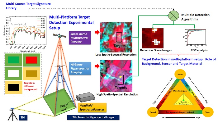
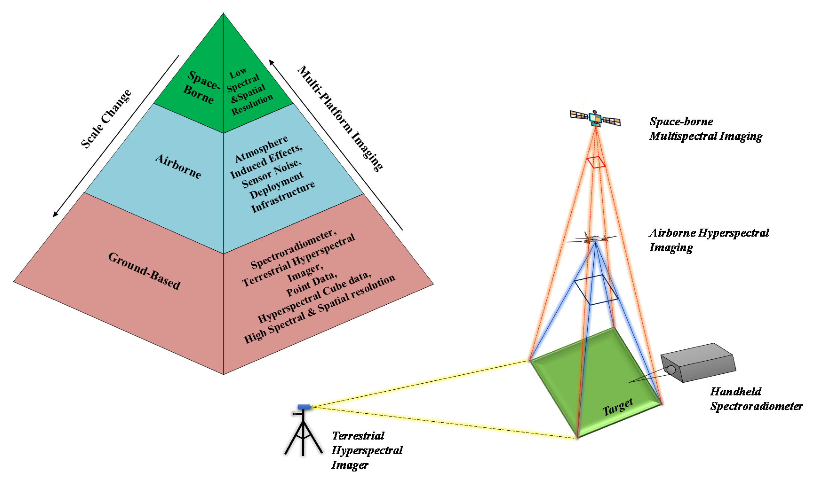
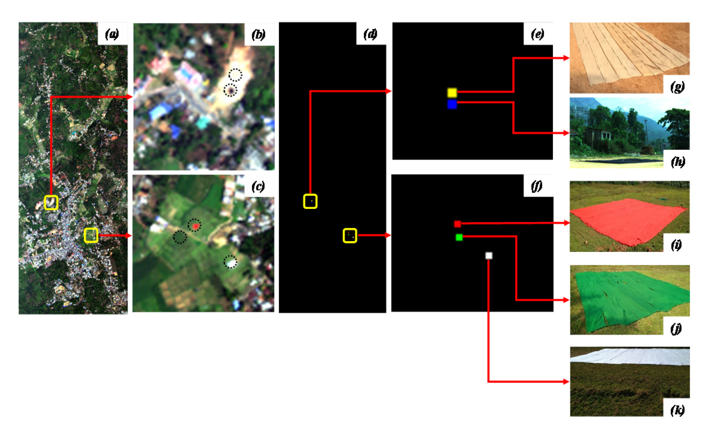
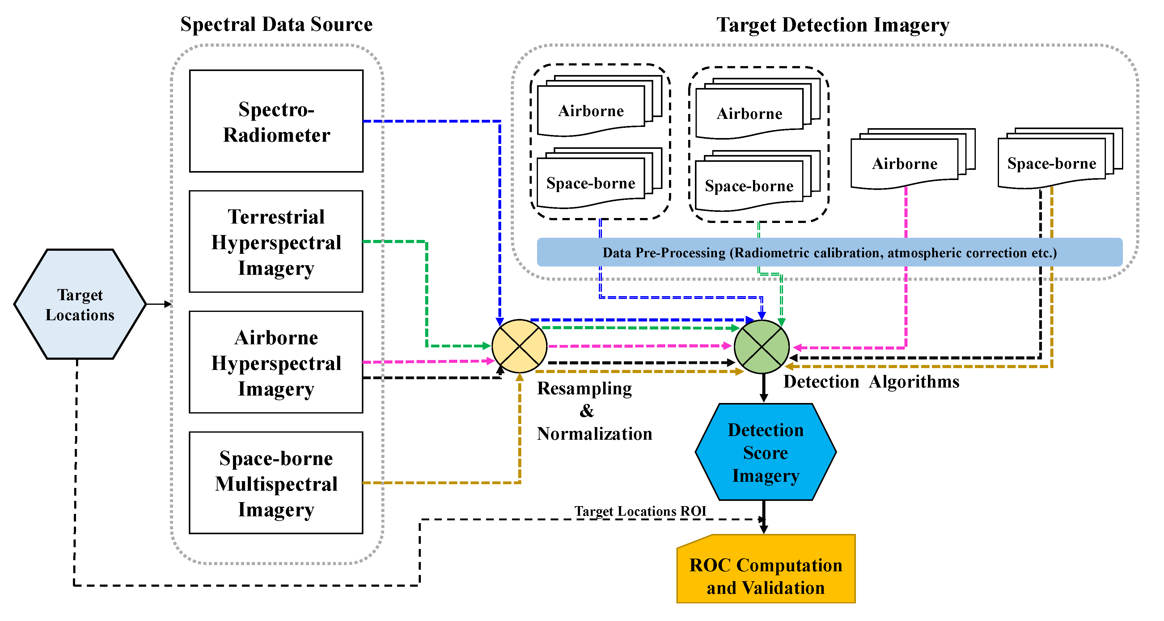
2.1. Experimental Design

The conceptual design of the experimental setup is shown in Figure 1.

The experimental set up consisted of positioning five targets of different artificial thin-sheet materials of different colors (base material: nylon and cotton), each of the size 10 m × 10 m (Figure 2). For ease of referencing throughout the paper, we designate a distinct name for each target used in this study in

Table 1. Target materials and naming convention used in the paper.

Target Material	Target Name
Green nylon sheet	N1G
Red nylon sheet	N2R
White cotton sheet	C1W
Yellow nylon sheet	N3Y
Black nylon sheet	N4B

. The third letter in the name of a target indicates the color of the target (G: green, R: red, W: white, Y: yellow, B: black).

Out of the five different target materials, we positioned three on natural grass and vegetation features as the background, and two on reflective soil background. To introduce a moderate degree of background resemblance to natural camouflage in the visible spectral range of the electromagnetic spectrum, we positioned two targets (N1G and N3Y) on the grass and soil background. To assess the target detection of materials with broadly similar spectral reflectance characteristics, we chose multiple targets with a single base material but in different colors. Ensuring an overlapping areal extent of the imagery from both the airborne and space-borne platforms, we extracted a subset of the data acquired. The datasets maintain SNR ratio close to one in a million for different scene elements under the different spatial-spectral variabilities of materials in the scene. A true color composite of the airborne hyperspectral imagery marked with footprints of the targets and the corresponding ground truth imagery are shown in Figure 2.

2.2. Data Pre-Processing

2.2.1. Reference Spectral Data Sources and Pre-Processing

On 20th March 2018, we acquired multi-platform remote sensing data: ground-based terrestrial hyperspectral imager (THI), airborne hyperspectral imager (AVIRIS-NG) [17], and the space-borne multispectral sensor (Sentinel-2). The THI is a push-broom hyperspectral imager (Headwall Photonics Inc., USA) mounted on a movable tripod-kind of the platform. The THI acquires hyperspectral imagery in the VNIR region (40–1000 nm) at about 1nm spectral resolution. In the present setup, a nominal spatial resolution of 1 cm further approximated to 20 cm across the targeted area was acquired in a nadir to oblique view. The AVIRIS-NG hyperspectral sensor was operated to acquire imagery with 4 m spatial resolution and 5 nm spectral resolution in the 400–2500 nm spectral range. The airborne hyperspectral data acquisition was part of the NASA and ISRO research collaboration for the HYPSIRI hyperspectral satellite [18]. The satellite imagery was acquired about one hour before the acquisition of airborne hyperspectral imagery. Apart from the spectral imagery, we collected point-based in-situ hyperspectral reflectance measurements using a field spectroradiometer (Spectra Vista Corporation, HR-1024i, USA) on the target materials as per the standard procedures [19]. The in-situ measurements are considered pure spectral signatures of the target materials, free of atmosphere, and target–surface–neighborhood interactions. Plots of in-situ reference spectral signatures of the target materials are shown in Figure 3. There are two sources of ground-based target reference spectra, ground-based hyperspectral imagery (THI) (reference in-situ pixels), and the point-based in-situ spectral reflectance from spectroradiometer. Since the THI collects hyperspectral imagery at a finer spatial resolution, we generated the reference target spectra by sampling target pixels corresponding to different places on the target materials. As the THI imager is sensitive to sensor noise beyond 900 nm, we used the THI data acquired in the spectral range 400 nm to 900 nm. After the initial pre-processing, which included the calibration using the concurrent measurements acquired on white reference panels, all the spectral data were convolved and resampled using the sensor response function (SRF) of the respective sensor for analysis across the datasets.

2.2.2. Pre-Processing of Airborne and Spaceborne Imagery

The airborne AVIRIS-NG hyperspectral imagery was corrected for atmospheric distortions using the radiative transfer based Fast Line-of-sight Atmospheric Analysis of Spectral Hypercubes (FLAASH) model [20] and removed the noisy and uncalibrated spectral bands between 1348–1443 nm, 1804–1954 nm, 2485–2500 nm thus resulting in effective imagery with 370 spectral bands. The Sentinel-2 satellite acquires multispectral imagery at different spatial resolutions, 10 m, 20 m, and 60 m. We used the imagery acquired at 10 m and 20 m resolution corresponding to blue (490 nm), green (560 nm), red (665 nm), NIR(842 nm), and vegetation red edge (705 nm, 740 nm, 783 nm, 865 nm), SWIR(1610 nm, 2190 nm) bands of the sentinel-2 product respectively centered at the given wavelengths. Generating a vertically conforming surface reflectance data, we corrected the Sentinel-2 imagery for atmospheric distortions using the same model and sensor-surface hyper-parameters used for airborne imagery. The imagery acquired at 20 m spatial resolution was resampled to 10 m resolution to conform to other imagery datasets.

2.3. Experimental Implementation of Target Detection

An outline of the methodological process flow adopted for the study is shown in Figure 4. The ground position of the targets was recorded using a GPS device. Since the targets used in the experiments were considerably large, we designated the target footprint for the airborne imagery as a 16-pixel region of interest (ROI) and a 4-pixel ROI for space-borne imagery on similar basis as suggested in [15]. It must be noted that, due to different sensor resolutions (4 m and 10 m for airborne and space-borne sensor respectively) and imaging geometry, target ROI for airborne imagery contains both full pixel as well as sub-pixel targets, while, target ROI for space-borne imagery contains predominantly sub-pixel targets. Since part of our aim was to evaluate the target detection possibility from multiple platforms, the input signal sources for the detector algorithms were collected from various sensors, as shown in Figure 4. We visualize three different scenarios: (i) the use of ground-based target spectra for detection from airborne and space-borne imagery, (ii) the use of ground-based hyperspectral imager target spectra for detection from airborne and space-borne imagery, and (iii) the use of airborne based target spectra for detection from space-borne imagery which can represent the essence of target detection problem from multiple civil and defense application perspectives.

Target Detection Algorithms

Apart from the target’s optical-spectral features and environmental settings, the target detection problem has two other primary perspectives—appropriate spectral imagery and detection algorithms. Given the applicable nature of spectral imagery, target recognition and identification are substantially controlled by the nature of algorithms used for target detection. While the development of advanced target detection algorithms is not within the purview of this study, it would be valuable to analyze the variations of target detections as a function of the detection algorithm. We, therefore, studied the target detection in the datasets with popular detection algorithms available in the literature, evaluating the quality and sensitivity of the target detections based on the algorithms used.

We considered six different detection algorithms: spectral angle mapper (SAM), matched filter (MF), adaptive cosine estimator (ACE), constrained energy minimization (CEM), orthogonal subspace projection (OSP), and transformed constrained interference minimization filter (TCIMF) for evaluating the target detections on the experimental dataset. The SAM, MF, ACE, and CEM are spectral detectors and hence do not require any prior knowledge of the background. However, OSP and TCIMF require prior scene background characterization. Typically, this is approached heuristically estimating the number of distinct background materials or endmembers. The number of distinct background materials represents the complexity of the scene and hence is a scene dependent parameter. We used the SMACC algorithm [21] for the background endmembers estimation. The detection performance of the OSP and TCIMF was evaluated for three different numbers (5, 10, and 15 endmembers) of background endmembers. We present a summary of the mathematical aspects of target detection and the formulation of different target detection algorithms used in this study.

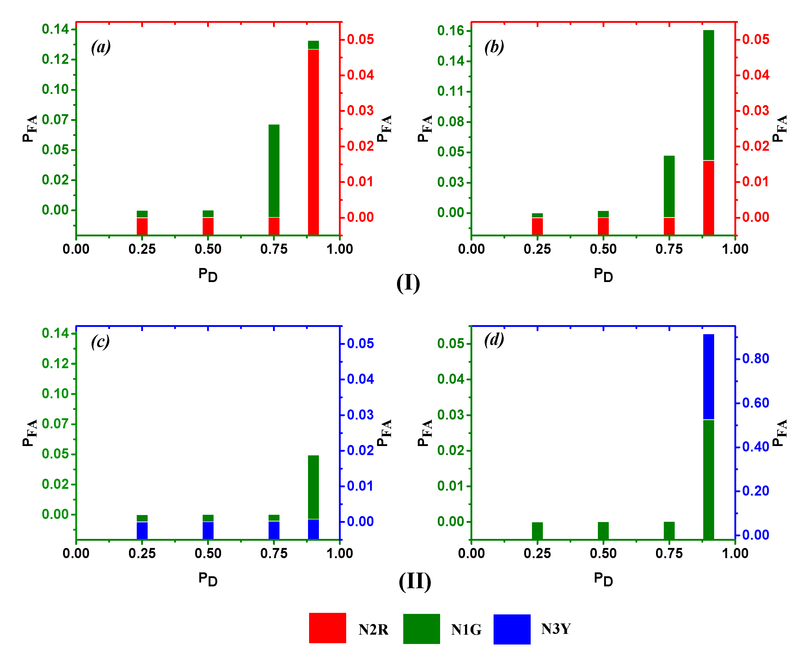
2.4. Quantitative Description of Target Detection Algorithms

The taxonomy of detection algorithms depends on various factors such as target-pixel occupancy (full pixel vs. sub-pixel target), considerations for spectral variability (either for target or background), and modeling the combination of pixel and sub-pixel targets [22]. Given an image ${\chi }_{\left(m,n\right)}$ having $k$ spectral channels and $m\times n$ pixels such that each pixel ${\mathrm{x}}_i$ = ${\left\{x_1,x_2,x_3,x_4\dots x_k\right\}}^t\in {\mathrm{X}}_{k,mn}$, target detection is formulated as a hypothesis testing problem. Mathematically, target detection can be expressed as a binary hypothesis testing problem:

$$\begin{gathered} {\mathrm{H}}_0\left(\mathrm{Null}\mathrm{Hypothesis}\right){\mathrm{x}}_i:\mathrm{noise}\left(\mathrm{Target}\mathrm{absent}\right), \\ {\mathrm{H}}_1\left(\mathrm{Alternate}\mathrm{Hypothesis}\right)x_i:\mathrm{Target}. \end{gathered}$$

Assuming a multivariate normal distribution for target and background, the target detection is represented as a hypothesis testing:

$$\begin{gathered} {\mathrm{H}}_0:\mathrm{x}=\mathrm{n} \\ {\mathrm{H}}_1:\mathrm{x}=\mathrm{s}+\mathrm{n} \end{gathered}$$

(1)

where $\mathrm{s}$ is the known target spectrum and $\mathrm{n}$ is the noise or background with mean vector ‘$\mathrm{m}$’ and covariance matrix $\mathrm{C}$ such that $\mathrm{n}~N\left(\mathrm{m},\mathrm{C}\right)$. Since the target and background are assumed to follow a multivariate normal distribution, the probability density function $p\left(x,\mathsf{\theta }\right)$ for a $\mathrm{k}$-dimensional Gaussian vector $x$ is given by:

$$p\left(\mathrm{x},\mathsf{\theta }\right)=\frac{1}{{\left(2\pi \right)}^{\mathrm{k}/2}{\left|\mathrm{C}\right|}^{1/2}}\exp \left\{-\frac{1}{2}{\left[\mathrm{x}-\mathrm{m}\right]}^T{\mathrm{C}}^{-1}\left[\mathrm{x}-\mathrm{m}\right]\right\}.$$

(2)

At a given false alarm rate (Neyman–Pearson criterion), the probability of detection is maximized by using a likelihood ratio (LR) type of detectors [23] expressed as:

$$l\left(\mathrm{x}\right)=\frac{\mathrm{p}\left({\mathrm{x}|\mathrm{H}}_1\right)}{\mathrm{p}\left({\mathrm{x}|\mathrm{H}}_0\right)}\begin{array}{c}{\mathrm{H}}_1\\ \gtrless \\ {\mathrm{H}}_0\end{array}\mathsf{\eta }$$

(3)

where $\mathsf{\eta }$ is the threshold. If $l\left(\mathrm{x}\right)$ is greater than $\mathsf{\eta }$, then alternate hypothesis (target-present) is declared true. Equation (1) describes the basic statistical model in case of a full pixel under the ideal assumption of the same covariance estimate for both target and background. However, at times target pixel gets mixed up due to the targets being spatially unresolved. In such cases the appropriate statistical model (also known as replacement model) is:

$$\begin{gathered} {\mathrm{H}}_0:\mathrm{x}=\mathrm{n} \\ {\mathrm{H}}_1:\mathrm{x}=\mathsf{\alpha }\mathrm{s}+\mathsf{\beta }\mathrm{n} \end{gathered}$$

(4)

where $\mathrm{x}~N\left(0,\mathrm{C}\right)$ under ${\mathrm{H}}_0$ and $\mathrm{x}~N\left(\mathsf{\alpha }\mathrm{s},{\mathsf{\beta }}^2\mathrm{C}\right)$; $\mathsf{\alpha }$ refers to the fraction fill of the target or abundances if $\mathrm{s}$ represents a matrix containing endmembers.

Our experimental study involved both kinds of the detection problem, full pixel and sub-pixel targets. Several full and sub-pixel target detection algorithms such as spectral angle mapper (SAM) [24], matched filter (MF) [25], constrained energy minimization (CEM) [26], adaptive cosine estimator (ACE) [27], orthogonal subspace projection (OSP) [28], and target constrained interference minimization filter (TCIMF) [29] were implemented for the detection of targets in this experiment.

Spectral Angle Mapper (SAM):

Modifying the signal model given by Equation (1), we have the hypothesis testing:

$$\begin{gathered} {\mathrm{H}}_0:\mathrm{x}=\mathrm{n} \\ {\mathrm{H}}_1:\mathrm{x}=\mathsf{\alpha }\mathrm{s}+\mathrm{n} \end{gathered}$$

(5)

where $\mathsf{\alpha }$ represents the strength of the target signal in the acquired imagery, $\mathrm{n}~N\left(0,{\sigma }^2\mathrm{I}\right)$ with ${\sigma }^2$ being variance. We estimated $\mathsf{\alpha }$ using the maximum likelihood estimate (MLE) under the modified signal model as:

$$\frac{\partial p\left({\mathrm{x}|\mathrm{H}}_1\right)}{\partial \alpha }=\frac{\partial }{\partial \alpha }\left\{\exp \left(\frac{-1}{2}{\left(\mathrm{x}-\alpha s\right)}^{\mathrm{T}}\left(\mathrm{x}-\alpha s\right)\right)\right\}.$$

(6)

Solving Equation (5), we obtained the MLE estimate of $\mathsf{\alpha }$ as follows:

$$\widehat{\mathsf{\alpha }}=\frac{{\mathrm{s}}^{\mathrm{T}}\mathrm{x}}{{\mathrm{s}}^{\mathrm{T}}\mathrm{s}}.$$

(7)

It is usual to estimate the variance (${\sigma }^2$) from the image pixel, i.e., pixel under test given by ${\widehat{\sigma }}^2={\mathrm{x}}^{\mathrm{T}}\mathrm{x}$. Substituting the estimated parameters in Equation (3) and taking the log-likelihood of the distribution functions, the test statistic is given by:

$$r\left(\mathrm{x}\right)=\ln \left(\frac{\mathrm{p}\left({\mathrm{x}|\mathrm{H}}_1\right)}{\mathrm{p}\left({\mathrm{x}|\mathrm{H}}_0\right)}\right)=\frac{{({\mathrm{s}}^{\mathrm{T}}\mathrm{x})}^2}{\left({\mathrm{s}}^{\mathrm{T}}\mathrm{s}\right)\left({\mathrm{x}}^{\mathrm{T}}\mathrm{x}\right)}.$$

(8)

We reframed the Equation (5) to represent the test statistic known as spectral angle mapper (SAM) as:

$$r_{SAM}\left(\mathrm{x}\right)={\cos }^{-1}\left[\frac{{\mathrm{s}}^T\mathrm{x}}{\sqrt{\left({\mathrm{s}}^T\mathrm{s}\right)\left({\mathrm{x}}^T\mathrm{x}\right)}}\right].$$

(9)

SAM is one of the widely used algorithms in hyperspectral remote sensing for solving spectral classification and matching problems and works on the assumption of a zero-mean and white background. Geometrically, SAM measures the similarity between two n-dimensional vectors based on the cosine of the angle between two vectors.

Matched Filter (MF):

The assumption of a zero-mean and white background is unrealistic for target detection in a world scenario. Allowing a moderate degree of flexibility in this aspect, the MF allows background representation with a normal distribution with finite mean and covariance. The signal model then becomes:

$$\begin{gathered} {\mathrm{H}}_0:\mathrm{x}=\mathrm{n} \\ {\mathrm{H}}_1:\mathrm{x}=\mathsf{\alpha }\mathrm{s}+\mathrm{n} \end{gathered}$$

(10)

where $\mathrm{n}~N\left(\mathrm{m},\mathrm{C}\right)$, and $\mathsf{\alpha }$ are the unknown parameters. For the given model, we have:

$$p\left(\mathrm{x}|{\mathrm{H}}_0\right)=\frac{1}{{\left(2\pi \right)}^{\mathrm{k}/2}{\left|\widehat{\mathrm{C}}\right|}^{1/2}}\exp \left\{-\frac{1}{2}{\left[\mathrm{x}-\widehat{\mathrm{m}}\right]}^T{\widehat{\mathrm{C}}}^{-1}\left[\mathrm{x}-\widehat{\mathrm{m}}\right]\right\}$$

(11)

$$p\left(\mathrm{x}|{\mathrm{H}}_1\right)=\frac{1}{{\left(2\pi \right)}^{\mathrm{k}/2}{\left|\widehat{\mathrm{C}}\right|}^{1/2}}\exp \left\{-\frac{1}{2}{[\mathrm{x}-\widehat{\mathsf{\alpha }}\mathrm{s}-\mathrm{m}]}^T{\widehat{\mathrm{C}}}^{-1}\left[\mathrm{x}-\widehat{\mathsf{\alpha }}\mathrm{s}-\widehat{\mathrm{m}}\right]\right\}$$

(12)

Applying the MLE estimation technique similar to Equation (6) we get:

$$\widehat{\mathsf{\alpha }}=\frac{{\mathrm{s}}^T{\widehat{\mathrm{C}}}^{-1}\left(\mathrm{x}-\widehat{\mathrm{m}}\right)}{{\mathrm{s}}^T{\widehat{\mathrm{C}}}^{-1}\mathrm{s}},\widehat{\mathrm{m}}=\frac{1}{\mathrm{N}}{\displaystyle \sum }_{i=1}^{\mathrm{N}}{\mathrm{x}}_i,\widehat{\mathrm{C}}=\frac{1}{\mathrm{N}}{\displaystyle \sum }_{i=1}^{\mathrm{N}}\left[{\mathrm{x}}_i-\widehat{\mathrm{m}}\right]{\left[{\mathrm{x}}_i-\widehat{\mathrm{m}}\right]}^{\mathrm{T}}.$$

(13)

Since the detector assumes an additive model, for $\mathsf{\alpha }=1$ under the null hypothesis, we have x = s + m, which is incorrect. In addition, α, by definition, is not constrained to be positive and may cause negative test statistics (Eismann et al., 2009). Correcting for these two problems and using the estimates from Equation (13), we can express MF score $r$ as:

$$r_{MF}\left(\mathrm{x}\right)=\frac{{(\mathrm{s}-\widehat{\mathrm{m}})}^T{\widehat{\mathrm{C}}}^{-1}\left(\mathrm{x}-\widehat{\mathrm{m}}\right)}{\sqrt{{\left(\mathrm{s}-\widehat{\mathrm{m}}\right)}^T{\widehat{\mathrm{C}}}^{-1}\left(\mathrm{s}-\widehat{\mathrm{m}}\right)}}.$$

(14)

Adaptive Cosine Estimator (ACE):

Modifying the Equation (4) to include a scale factor $\mathsf{\beta }$ yields the following replacement model:

$$\begin{gathered} {\mathrm{H}}_0:\mathrm{x}=\mathsf{\beta }\mathrm{n} \\ {\mathrm{H}}_1:\mathrm{x}=\mathrm{x}=\mathsf{\alpha }\mathrm{s}+\mathsf{\beta }\mathrm{n} \end{gathered}$$

(15)

where $n~N\left(0,\mathrm{C}\right)$ and $\mathsf{\alpha }$, $\mathsf{\beta }$ are the unknown parameters. The above model is similar to Kelly’s detector (Kelly, 1986), except for the introduction of an unknown parameter $\mathsf{\beta }$ in the null hypothesis. The ACE detector was derived based on the assumption of different covariance estimates (${\widehat{\mathrm{C}}}_0,{\widehat{\mathrm{C}}}_1$) under the null and alternate hypotheses. It is assumed that the data under the null hypothesis correspond to training data for noise/background estimation and pixel under test (under the alternative hypothesis) is the testing data. Maximizing the joint probability density function of the training and test data yields the following estimates:

$$\widehat{\mathsf{\alpha }}=\frac{{\mathrm{s}}^T{\widehat{\mathrm{C}}}^{-1}\mathrm{x}}{{\mathrm{s}}^T{\widehat{\mathrm{C}}}^{-1}\mathrm{s}},{\widehat{\mathsf{\beta }}}_0^2=\frac{\mathrm{N}-\mathrm{k}+1}{\mathrm{Nk}}{\mathrm{x}}^{\mathrm{T}}{\widehat{\mathrm{C}}}^{-1}\mathrm{x},{\widehat{\mathsf{\beta }}}_1^2=\frac{\mathrm{N}-\mathrm{k}+1}{\mathrm{Nk}}{\left(\mathrm{x}-\widehat{\mathsf{\alpha }}\mathrm{s}\right)}^{\mathrm{T}}{\widehat{\mathrm{C}}}^{-1}\left(\mathrm{x}-\widehat{\mathsf{\alpha }}\mathrm{s}\right),$$

and

$${\widehat{\mathrm{C}}}_0=\frac{1}{\mathrm{N}+1}\left[\frac{1}{{\mathsf{\beta }}_0^2}{\mathrm{xx}}^{\mathrm{T}}+\mathrm{N}\widehat{\mathrm{C}}\right],{\widehat{\mathrm{C}}}_1=\frac{1}{\mathrm{N}+1}\left[\frac{1}{{\mathsf{\beta }}_1^2}\left(\mathrm{x}-\mathsf{\alpha }\mathrm{s}\right){\left(\mathrm{x}-\mathsf{\alpha }\mathrm{s}\right)}^{\mathrm{T}}+\mathrm{N}\widehat{\mathrm{C}}\right]$$

(16)

where ${\widehat{\mathsf{\beta }}}_0$, ${\widehat{\mathrm{C}}}_0$, ${\widehat{\mathsf{\beta }}}_1$, ${\widehat{\mathrm{C}}}_1$ are the estimates under the null and alternate hypothesis, respectively. Plugging the derived estimates in the general form of log-likelihood ratio test detector (Equation (3)), we get the ACE score $r$ as:

$$r_{\mathrm{ACE}}\left(\mathrm{x}\right)=\frac{{\left({\mathrm{s}}^{\mathrm{T}}{\widehat{\mathrm{C}}}^{-1}\mathrm{x}\right)}^2}{({\mathrm{s}}^{\mathrm{T}}{\widehat{\mathrm{C}}}^{-1}\mathrm{s})\left({\mathrm{x}}^{\mathrm{T}}{\widehat{\mathrm{C}}}^{-1}\mathrm{x}\right)}.$$

(17)

Constrained Energy Minimization (CEM):

The aforementioned spectral detectors assume the target and background subspace to follow a particular statistical distribution. Based on the assumed distribution function, we usually derive the parameters of the distribution function. The assumption of background conformity to a statistical distribution may lead to ambiguous results if the target or background is different from the assumed statistical function. In such situations, it is desirable to design a detector that does depend upon the target–background distribution function and eliminates the interferer from the target signal. The CEM is one such detector and is functionally equivalent to a finite impulse response (FIR) filter that minimizes the detector output for the background pixels.

Given an image ${\chi }_{\left(m,n\right)}$ with $k$ spectral channel and $\mathrm{N}$ pixels such that each pixel $x_i$= ${\left\{x_1,x_2,x_3,x_4\dots x_{\mathrm{k}}\right\}}^t\in {\mathrm{X}}_{\mathrm{k}\times \mathrm{N}}$, the average energy of the FIR filter output can be written as:

$$\begin{gathered} \frac{1}{\left(\mathrm{N}\right)}\left\{{{\displaystyle \sum }}_{i=1}^{\mathrm{N}}{\varphi }_i{}^2\right\}=\frac{1}{\left(\mathrm{N}\right)}\left\{{{\displaystyle \sum }}_{i=1}^{\mathrm{N}}{({\mathrm{x}}_i{}^T\mathrm{W})}^T({\mathrm{x}}_i{}^T\mathrm{W})\right\}, \\ ={\mathrm{W}}^T\left\{\frac{1}{\mathrm{N}}{{\displaystyle \sum }}_{i=1}^{\mathrm{N}}{\mathrm{x}}_i{\mathrm{x}}_i{}^T\right\}\mathrm{W}={\mathrm{W}}^T\mathrm{RW} \end{gathered}$$

(18)

where $\varphi =({\mathrm{x}}_i{}^T\mathrm{W})$ is the filter output for the pixel vector ${\mathrm{x}}_i$, $\mathrm{W}={\left(w_1,w_2,w_3,w_4\dots w_k\right)}^T$ is the weight vector for the designed filter, and R is the k-dimensional background correlation matrix. The CEM problem statement then becomes a constraint optimization problem, i.e., $\underset{\mathrm{w}}{\min }\left({\mathrm{W}}^T{\mathrm{R}}_{\mathrm{k}\times \mathrm{k}}\mathrm{W}\right)$ subject to ${\mathrm{s}}^{\mathrm{T}}\mathrm{W}=1$. The detection problem is solved using the Lagrange’s multiplier method to solve the constrained optimization problem to get the CEM score $r$ as:

$$r_{CEM}\left(\mathrm{x}\right)=\frac{\left({\mathrm{s}}^{\mathrm{T}}{\mathrm{R}}^{-1}\mathrm{s}\right)}{{\left({\mathrm{R}}^{-1}\mathrm{s}\right)}^{\mathrm{T}}\mathrm{x}}.$$

(19)

Orthogonal subspace projection (OSP):

In most of the practical hyperspectral target detection problems, the target size is less than a full pixel. In such cases, spectral mixture models are useful to estimate the material abundances. The OSP assumes a linear mixture model expressed as:

$$\mathrm{x}=\mathrm{M}\mathsf{\alpha }+\mathrm{n}$$

(20)

where $\mathrm{M}$ is a matrix of target/known spectral signatures, $\mathsf{\alpha }$ is abundance, and $\mathrm{n}$ is the noise. The OSP begins by first separating the desired target and unknown target and then projecting desired targets orthogonally to undesired/interferer target space. Mathematically OSP is given by:

$$r_{OSP}={\mathrm{d}}^{\mathrm{T}}{P}_{\mathrm{U}}^{\perp }\mathrm{x}$$

(21)

where d is the desired target, $P_{\mathrm{U}}^{\perp }$ is the projection operator which projects the image pixel to space orthogonal to $\mathrm{U}$ (undesired targets/interferer) given as $P_{\mathrm{U}}^{\perp }={\mathrm{I}}_{\mathrm{k}\times \mathrm{k}}-{\mathrm{UU}}^{\#}$, ${\mathrm{U}}^{\#}$ is the pseudo inverse of U and given as (U^TU)⁻¹U^T, and ${\mathrm{I}}_{\mathrm{k}\times \mathrm{k}}$ is the identity matrix.

Target constrained interference minimization filter (TCIMF):

In this approach, the image is assumed to be a combination of three signal components, i.e., desired (targets), undesired (unwanted/background), and interferer component. Like the CEM, the desired component is accentuated while suppressing the interference signal. The TCIMF is a theoretical superset of CEM and capable of detecting multiple targets at once, unlike CEM and OSP. Mathematically, TCIMF score is given as:

$$r_{\mathrm{TCIMF}}\left(\mathrm{x}\right)={\left\{\frac{{\mathrm{R}}_{\mathrm{k}\times \mathrm{k}}^{-1}\left[\mathrm{DU}\right]}{\left({\left[\mathrm{DU}\right]}^{\mathrm{T}}{\mathrm{R}}_{\mathrm{k}\times \mathrm{k}}^{-1}\left[\mathrm{DU}\right]\right)}\left[\begin{array}{c}{1}_{\mathrm{p}\times 1}\\ 0_{\mathrm{q}\times 1}\end{array}\right]\right\}}^T\mathrm{x}$$

(22)

where $\mathrm{D}=\left[{\mathrm{d}}_1,{\mathrm{d}}_2,\dots ,{\mathrm{d}}_{\mathrm{p}}\right]$ is the set of desired/known target signals, $\mathrm{U}=\left[{\mathrm{u}}_1,{\mathrm{u}}_2,\dots ,{\mathrm{u}}_{\mathrm{q}}\right]$ is the known background/unwanted signals in the image.

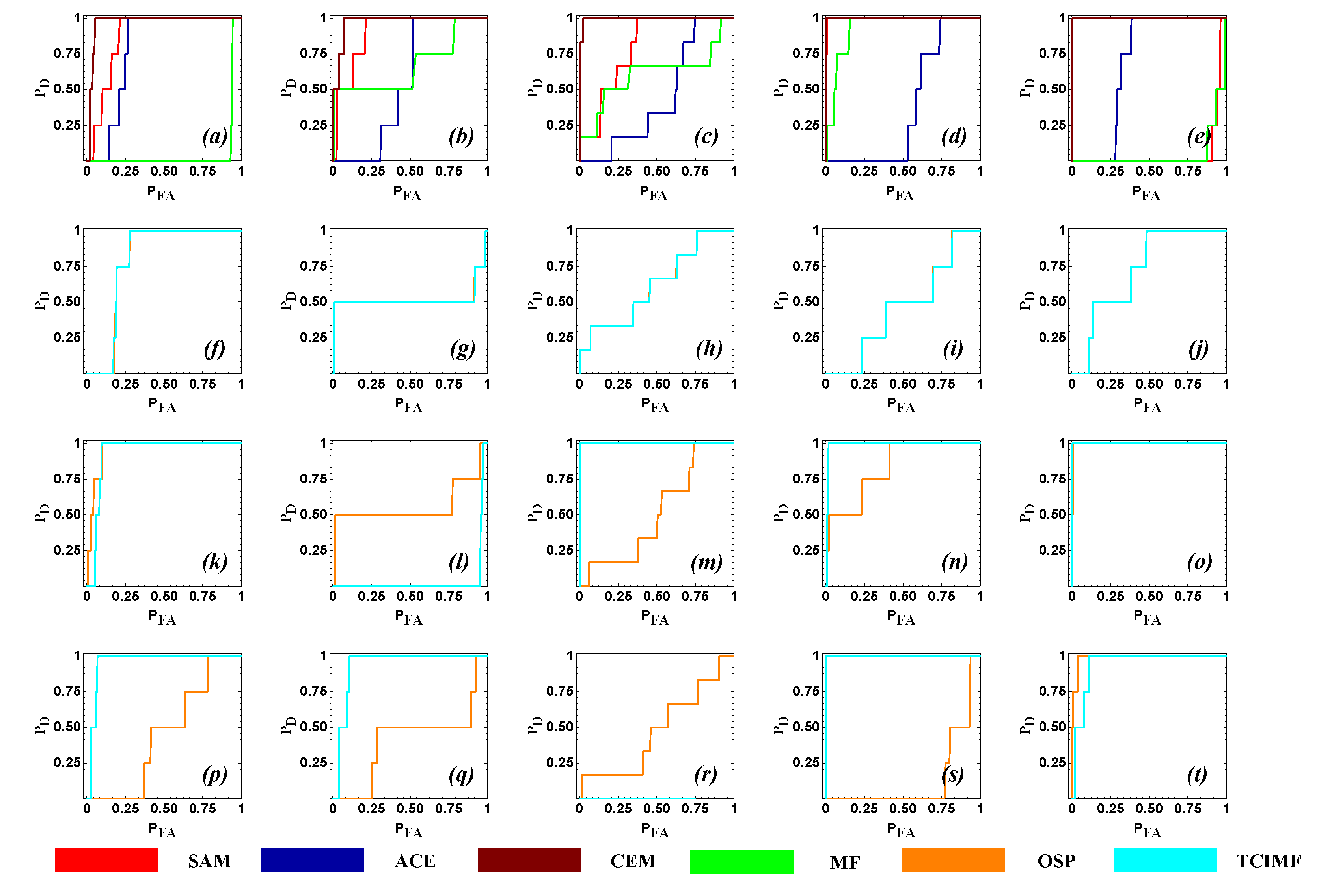
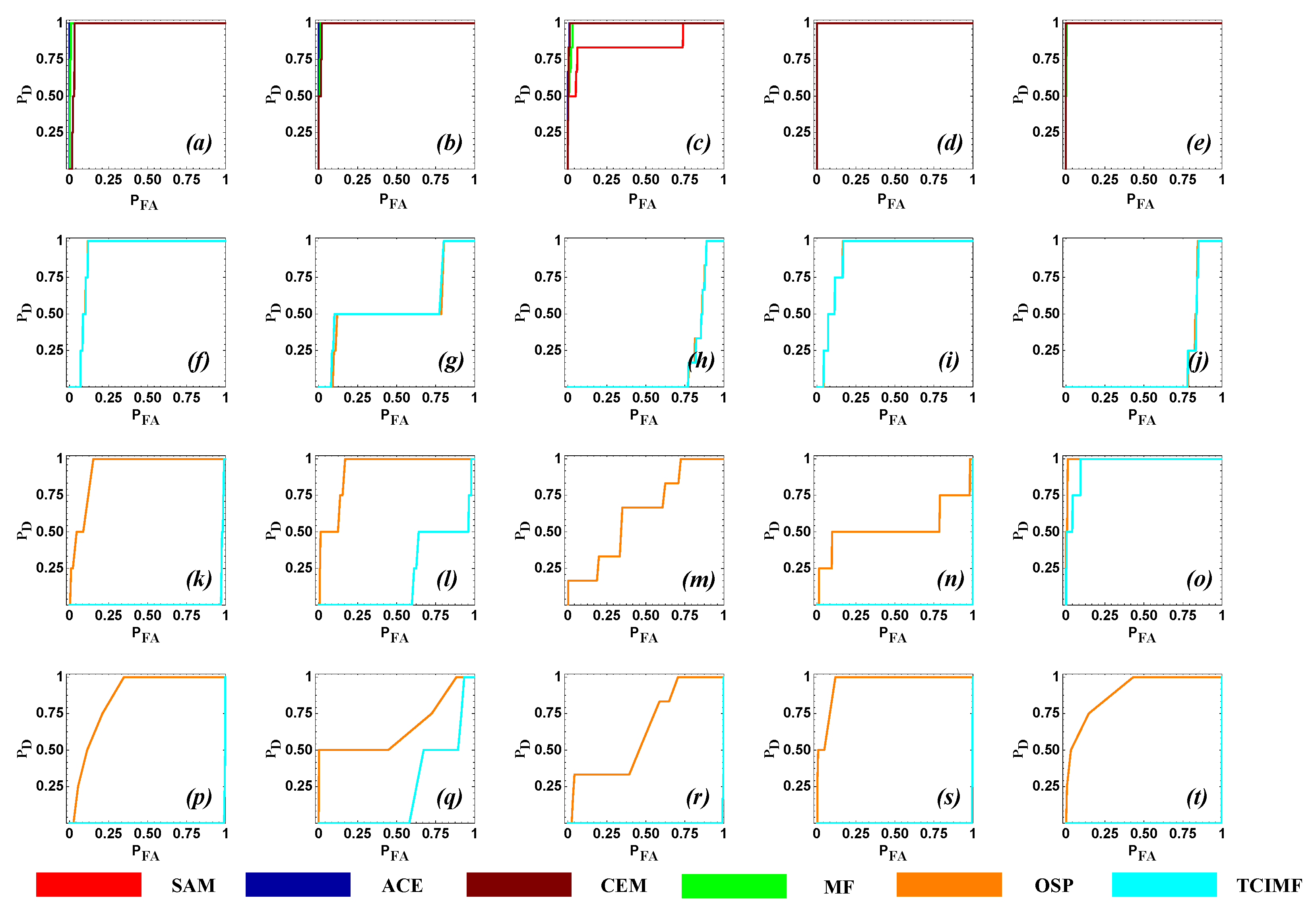
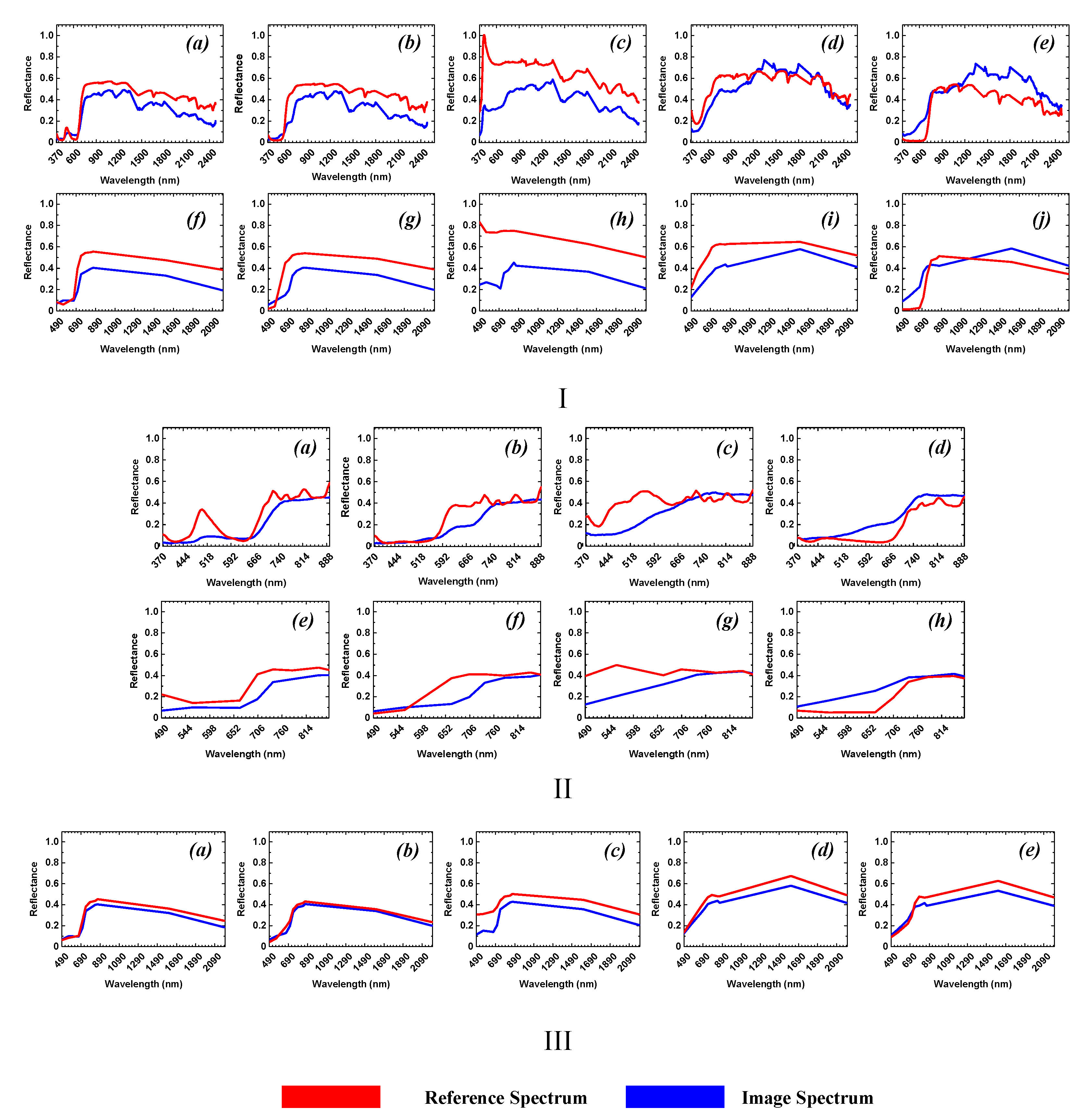
2.5. Validation, and Quantitative Spectral Analysis

The detection results from the different detection algorithms were compared against the ground truth map prepared for each case. Graph-based measures have been increasingly used for quantifying accuracy in various pattern recognition applications, especially in the cases of skewed class distributions [30]. By the rarity of occurrence, target detection is an approximation ofskewed class distribution [31]. We adopted the widely used ROC graphical measure for accuracy assessment. Based on the verified labels of the detections, ROC curves were drawn between the probability of false alarm (${\mathrm{P}}_{\mathrm{FA}}$) and the probability of detection (${\mathrm{P}}_{\mathrm{D}}$) expressed as:

$$\begin{gathered} {\mathrm{P}}_{\mathrm{D}}=\frac{\mathrm{Number}\mathrm{of}\mathrm{correctly}\mathrm{identified}\mathrm{target}\mathrm{pixels}}{\mathrm{Total}\mathrm{number}\mathrm{of}\mathrm{actual}\mathrm{target}\mathrm{pixels}} \\ {\mathrm{P}}_{\mathrm{FA}}=\frac{\mathrm{Number}\mathrm{of}\mathrm{pixels}\mathrm{identified}\mathrm{as}\mathrm{false}\mathrm{targets}}{\mathrm{Total}\mathrm{number}\mathrm{of}\mathrm{non}-\mathrm{target}\mathrm{pixels}}. \end{gathered}$$

(23)

The possibility and quality of target detections from multi-platform remote sensing imagery depend upon the existence and quantification of inherent spectral matching between target spectra from different platforms. Quantitative analysis of the spectral matching between the various combinations of reference target spectra and imaging platform deciphers the basis of target detections by detection algorithms. For each of the possible scenarios considered, we applied multiple spectral matching metrics: spectral angle (SA) [24], spectral information divergence (SID) [32], and spectral gradient angle (SGA) [33] on the spectral data extracted from the ground reference (ground hyperspectral imagery, and point-based spectral measurements) and the airborne and space-borne imagery. We present a brief description of the spectral matching metrics considered.

Consider any two n-dimensional vectors $\mathrm{P}={\left\{p_1,p_2,p_3,p_4\dots p_{\mathrm{n}}\right\}}^t$, and $\mathrm{Q}={\left\{q_1,q_2,q_3,q_4\dots q_{\mathrm{n}}\right\}}^t$.

The quantity’s spectral matching metrics SA, SID, and SGA are defined as:

$$\mathrm{SA}\left(\mathrm{P},\mathrm{Q}\right)={\cos }^{-1}\left(\frac{\langle P,Q\rangle }{{\parallel P\parallel }_2{\parallel Q\parallel }_2}\right)$$

(24)

where, 〈〉 denotes the dot product of two vectors and $\parallel .{\parallel }_2$ denotes the Euclidean norm of a vector.

$$\begin{gathered} \mathrm{SID}\left(\mathrm{P},\mathrm{Q}\right)=D\left(P\left|\right|Q\right)+D\left(Q\left|\right|P\right) \\ ={\Sigma }_{i=1}^n\left(\frac{p_i}{{\Sigma }_{j=1}^n{p}_j}-\frac{q_i}{{\Sigma }_{j=1}^n{q}_j}\right)\left(\log (\frac{p_i}{{\Sigma }_{j=1}^n{p}_j})-\log (\frac{q_i}{{\Sigma }_{j=1}^n{q}_j})\right), \end{gathered}$$

(25)

where $D\left(P\parallel Q\right)$ and $D\left(Q\parallel P\right)$ are called the relative entropy of Q with respect to P and relative entropy of P with respect to Q, respectively.

SID is a probabilistic approach to measure the spectral similarity between two spectra. Each pixel is represented in the probabilistic space defined by their spectral histogram. Thus, the SID score is an indication of the behavioral difference in the probability distribution function of any two pixels. A score close to zero from the SA and SID indicates that the spectra are similar [26,34]. The spectral gradient angle can be expressed as:

$$\begin{gathered} \mathrm{SGA}\left(\mathrm{P},\mathrm{Q}\right)=\mathrm{SA}\left(abs\left(\mathrm{SG}\left(\mathrm{P}\right)\right),abs\left(\mathrm{SG}\left(\mathrm{Q}\right)\right)\right)\mathrm{and} \\ \mathrm{SG}\left(\mathrm{P}\right)=\left(p_2-p_1,p_3-p_2,\dots ,p_n-p_{n-1}\right), \end{gathered}$$

(26)

where $\mathrm{SG}\left(.\right)$ is the spectral gradient of a given vector. The SGA computes the change of slope of the pixel vectors and is thus invariant to illumination condition similar to SA; a lower value of SGA suggests closer matching of the spectra compared.

3. Results

Our experimental research set up was aimed at examining three critical perspectives in remote sensing-based target detection: (i) platform—the probability and consistency of target detection vis-à-vis platforms, (ii) reference target spectra—the relevance and level of acquiescence of cross-platform target reference spectra, and (iii) detection algorithm—the variation of detection due to detection algorithms. The first component was approached by quantifying the magnitude and patterns of variation of $P_D$ with the three levels of platforms considered. The second component was addressed by comparing the levels of target detection rates between two sets of reference target spectra generated: from the same dataset and the cross-platform dataset. The third perspective, the influence of algorithms on the detection results, was assessed by measuring the change in patterns and detection rates from the different detection algorithms considered. As different detection algorithms characterize scene background at varying levels of land cover composition, the sensitivity of detection rates relative to the scene complexity (characterized by the number of endmembers) and the contrast between the target and its neighborhood was also carried out. The spectral analysis assessing the matching or lack of it in the multi-platform target spectra, quantitative comparison of the ground-based target reference spectra with the image-based target spectra, was also performed using three different spectral matching metrics. We present the results organized based on the source of the target reference spectra. We considered target detection successful at detection probabilities of ($P_D$) of 100%, and 75%, recognizing the fact that the datasets encompass a wider range of spectral variability. The detection and false alarm rates from different combinations of the platforms and algorithms are described in detail.

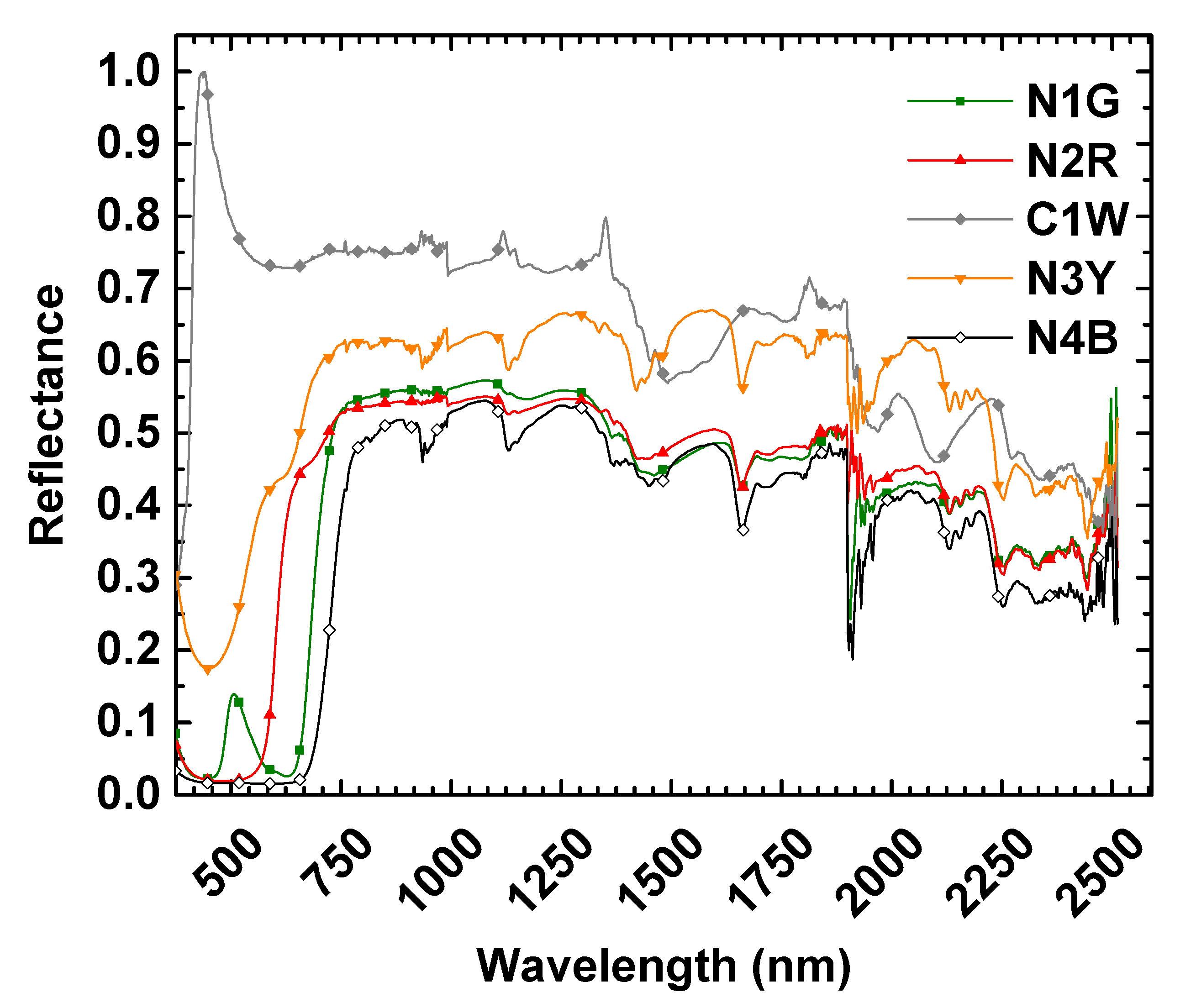
3.1. In-Situ Measurements as Reference Target Spectra

In this section, we present the results of target detection experiments when the in-situ reflectance measurements were used as the reference target spectra for target detection in airborne and space-borne imagery.

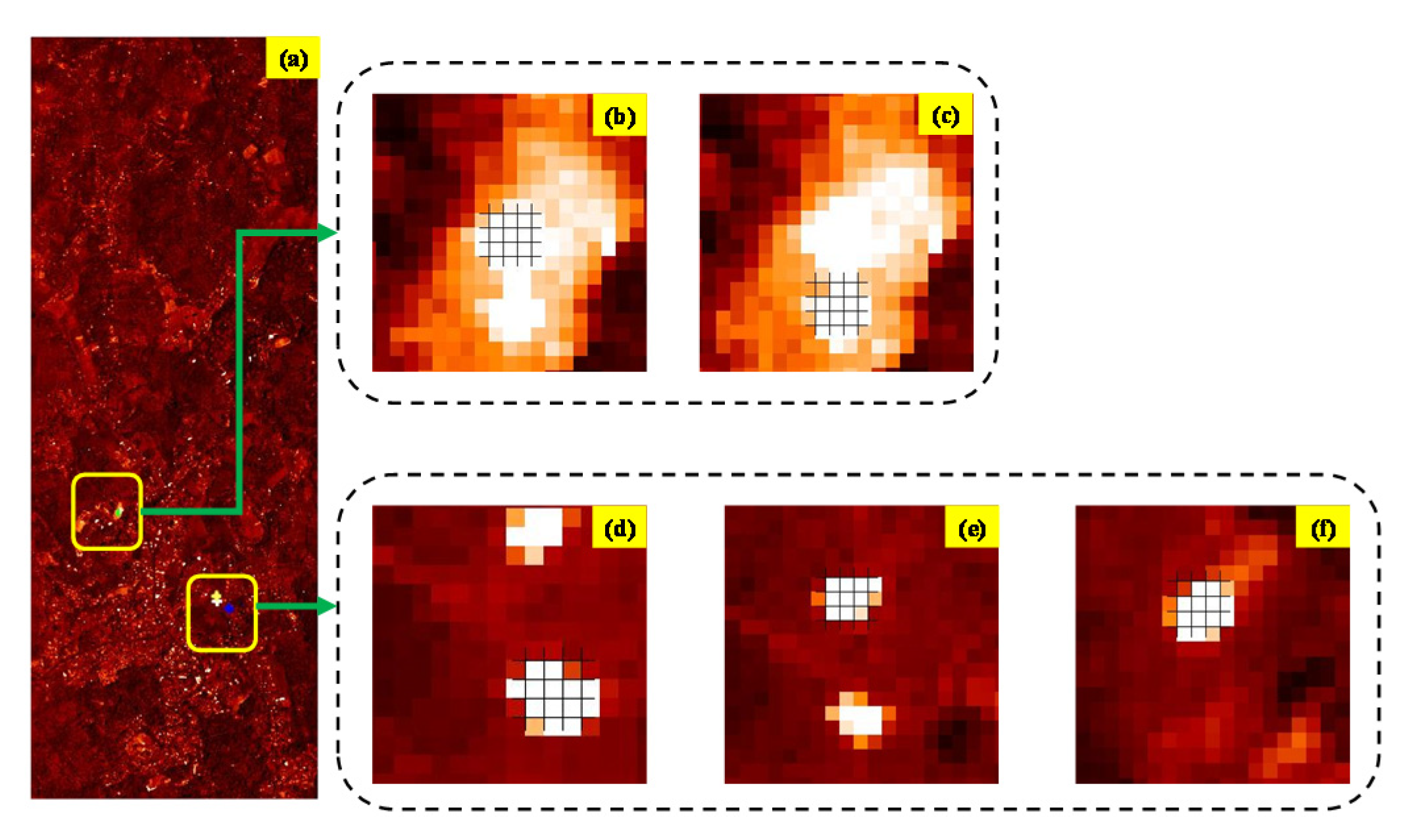
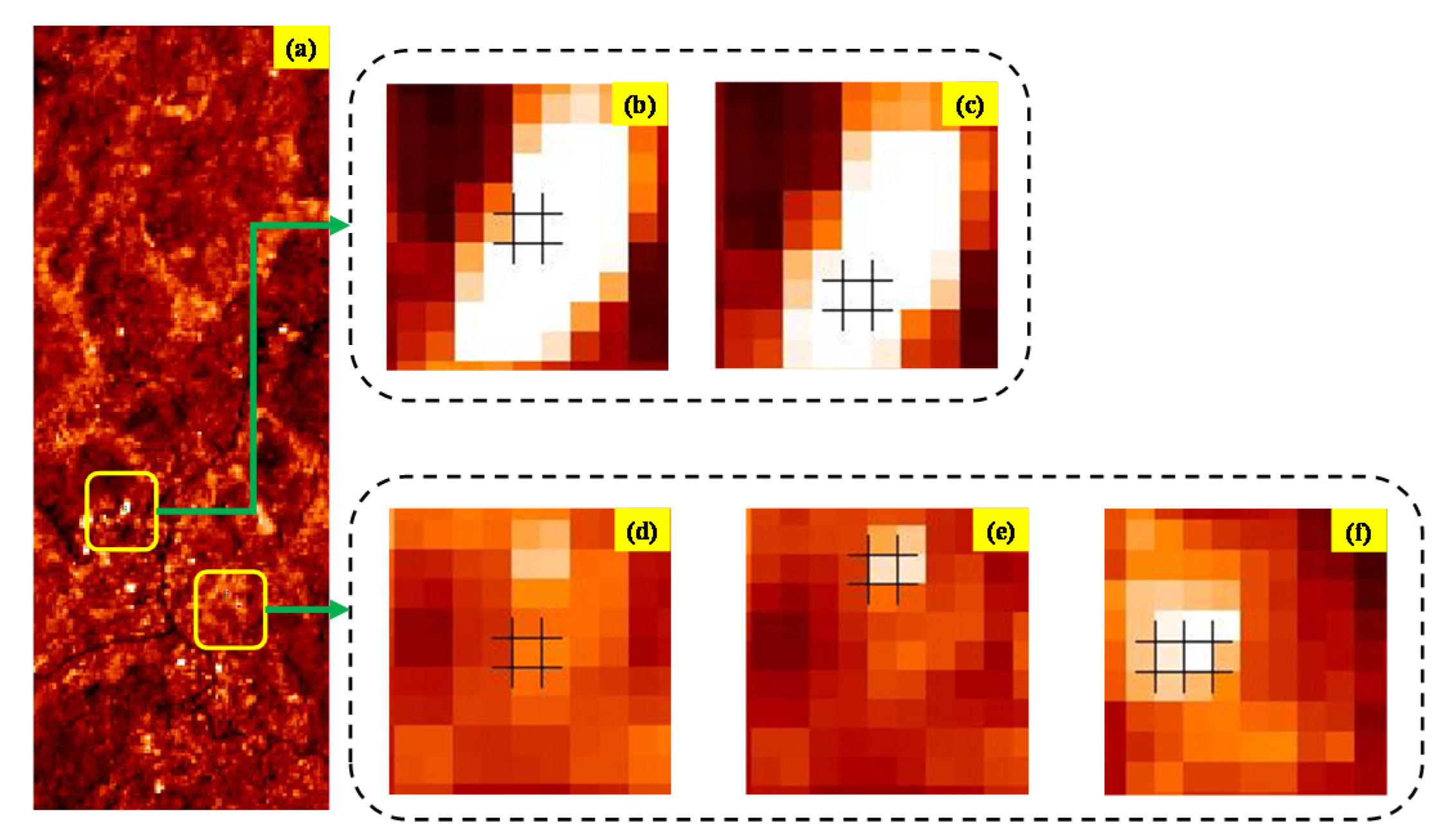
3.1.1. Target Detection in Airborne Hyperspectral Imagery

Results of the target detection in airborne hyperspectral imagery are summarized in Figure 5 and the corresponding representative detection score image in Figure 6. The detection score image is a raster image which contains a scalar value also known as score, corresponding to each pixel. The value represents the likelihood of the pixel for being flagged as target/non-target. Results indicate successful target detections for the different types of target materials, meeting the threshold detection rate at 100% threshold of $P_D$ for some materials. Overall, the detection rate is consistent across the types of materials. Except for SAM, all the detectors produced an average detection rate of 75% at nearly zero false alarm rate.

Detection rate vs. scene complexity: In contrast to the generally acceptable levels of detection rates for a broader approximation of scene-background, detection rates are substantially variable by the scene complexity, and target–neighborhood contrast. The detection rates are consistent and satisfy the lower threshold when the scene complexity was represented by five endmembers. When the scene complexity increased to represent 15 endmembers, the false alarm rate increased steeply, indicating substantial performance degradation in some detection algorithms. The rise in the false alarm rate was not uniform and varied by different classes of detection algorithms.

Identical materials vs. background contrast: It is expected that targets of identical material, even if of a different color or background, are recognizable ina hyperspectral imagery. Results indicate that the possibility of an identical base material target in a different color or on different background introduces substantial ambiguity in the quality of target detection. For example, at $P_D$ of 75%, the $P_{FA}$ from the CEM method is 0.0685, and $1.02\times {10}^{-4}$ respectively for the targets N2R and N1G placed on the same background. Similarly, the $P_{FA}$ for the ACE method is 0.017, and $2\times {10}^{-6}$ respectively for the N4B and N1G targets placed on different backgrounds. During the detection of the N2R, the N1G was also flagged as a potential target and vice-versa (see Figure 6d,e). The failure of the suppression of targets of identical color but of physically different materials is one of the challenging problems encountered for spectrally close materials. Apparently, by the absolute value, $P_{FA}$ is relatively low for considering the relevant target detections as ambiguous. However, when the corresponding $P_{FA}$ estimates are converted into actual pixel count, the certainty of detection seems to be far from the ideal case. For instance, for the N1G target, the CEM flags a false alarm of ~70 pixels distributed across the imagery. If the confidence of the detection rate is increased to 100% (i.e., ${\mathrm{P}}_{\mathrm{D}}$ = 100%), almost all the detectors show substantially lower detection results in terms of completeness of the targets. Overall, results suggest that, apart from the target–background interaction, the spectral contrast of targets play a substantial role in the detectability.

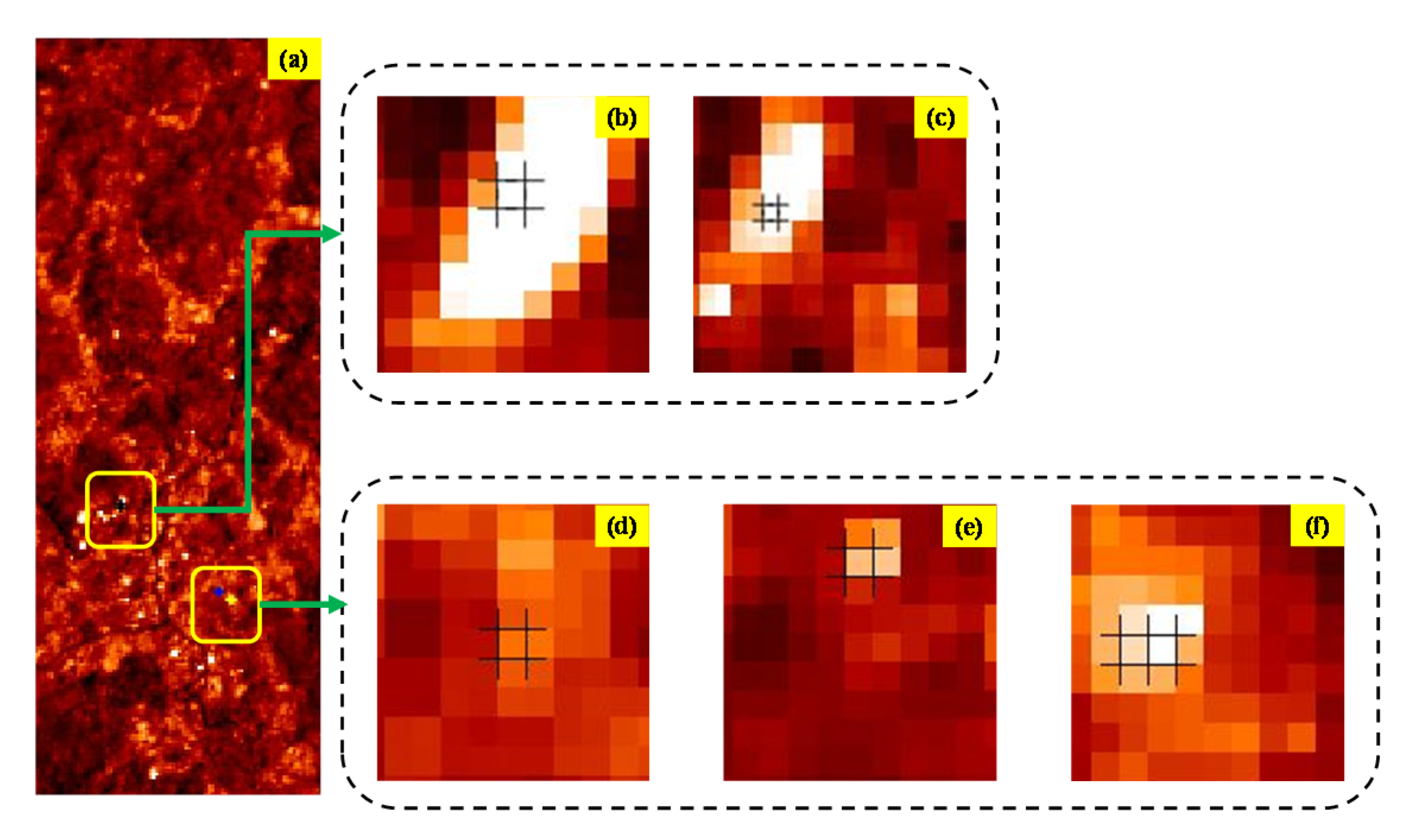
3.1.2. Target Detection in Spaceborne Remote Sensing Imagery

Results of the target detection in airborne hyperspectral imagery are summarized in Figure 7 and the corresponding representative detection score image in Figure 8. Due to coarse spectral and spatial resolutions and the substantially higher level of atmospheric influences, target detection in space-borne multispectral imagery is challenging compared to airborne hyperspectral imagery. Use of the in-situ reflectance measurements, considered a pure form of reference spectra, as target reference spectra, elicited no quantifiable spectral discrimination of target pixels in the satellite imagery. As evident from Figure 8, the detection scores and surrounding pixels are similar for targets N1G, N2R resulting in higher false alarm rates across all the algorithms (Figure 7). While the detection results included the pixels of targets, the apparent gross overestimation indicates the detection results to be unreliable. The detection algorithms either fail to detect or the respective false alarm rates are higher due to the relatively lesser number of estimated background endmembers. However, when the probability of detection was set at 75% and the scene complexity increased by representing with a large number of endmembers (10 or more), the sub-pixel target detection algorithms (e.g., CEM, TCIMF, Figure 7p) resulted in stable detection results. It is interesting to note that unlike target detection in airborne imagery, there was no change in the false alarm rate when the probability of detection was increased from 75% to 100%.

3.2. Ground-Based Hyperspectral Imagery (THI) as Reference Target Spectra

In remote sensing, in-situ or laboratory-based measurement of spectral reflectance is considered to be the pure form of the spectral signature of a material. While the relevance of the purity of spectral signature seems on a theoretically sound basis, the results presented in this section indicate that a pixel-based reference spectrum is a viable substitute to the in-situ spectra.

3.2.1. Target Detection in Airborne Hyperspectral Imagery

The results of target detection in airborne hyperspectral imagery and a representative detection score image are shown in Figure 9 and Figure 10. Results indicate the possibility of target detection, suggesting the existence of a spatially distinct spectral matching between the ground hyperspectral imagery and the airborne hyperspectral imagery. As shown in Figure 10e, in the case of the THI reference spectrum, suppression of similar but different targets (NIG suppressed when N2R was detected and vice-versa) is superior compared to the results from in-situ reference spectra (see Figure 6). However, the false alarm rate is higher compared to the extent and spatial distribution of the target pixels in the airborne hyperspectral imagery. This may be due to the limited in the spectral coverage (400–1000 nm), compared to the full optical spectrum of the airborne hyperspectral imagery (400–2500 nm). As the targets considered are inorganic artificial materials, spectral reflectance in the shortwave infrared region (1000–2500 nm) may provide characteristic spectral discrimination. Compared to the case of using in-situ reference target spectra, spectral matching based detection algorithms showed relatively better detection rate, consistent across the targets. In addition, contextually camouflaged targets were also detected, as indicated by the relatively higher scores of $P_D$ and negligible scores of $P_{FA}$.

The detection rate of the targets by background-characterization based algorithms is ambiguous. In-scene estimation of background material spectra was poor. For e.g., for the N3Y target, detection by TCIMF improved when the estimated number of background material increased from 5 to 15 but degraded at the same time for the N2R target. As observed, if the $P_D$ rate is required to be high ($P_D$ = 100%), detection rate from all the detectors is unacceptable for any practical system.

3.2.2. Target Detection in Spaceborne Remote Sensing Imagery

With the consideration of THI pixel spectra as target reference spectra, the results of target detection in space-borne multispectral imagery and a representative detection score image in Figure 11 and Figure 12, respectively. Similar to the results obtained with the point-based in-situ target reference spectra, the target detection in space-borne multispectral imagery is ambiguous across the types of targets. A couple of detection algorithms (e.g., CEM, OSP) produced detection scores meeting the threshold limit. However, the corresponding disproportionately high false alarm rate indicates that the detection is by chance.

3.3. Target Reference Spectra from the Airborne Hyperspectral Imagery

3.3.1. Target Detection in Airborne Hyperspectral Imagery

Target detection experiments were carried out on the airborne hyperspectral imagery and space-borne multispectral imagery using considering pixel-based spectra extracted from the airborne hyperspectral imagery as target reference spectra.

Figure 13 shows the target detection scores for the different types of targets in the airborne hyperspectral imagery. Targets were detected with detection scores exceeding 90% with negligible false alarm rates. The accurate detection of the lowest false alarm rates across the target types and detection algorithms indicate the possibility of consistent target detections in airborne hyperspectral imagery. However, the relatively higher rate of false positives for the contextually camouflaged targets suggests the dominance of local background–target interactions (as evident in Figure 14) on the radiance measurements. The limitations of the present suite of detection algorithms in discerning complex background–target interactions might also be a reason higher false alarm rate for detecting contextually camouflaged targets.

3.3.2. Target Detection in Spaceborne Multispectral Imagery

The target reference spectra extracted from the airborne hyperspectral imagery were transferred and convolved to space-borne level for target detection in the space-borne multispectral imagery. The detection results are summarized in Figure 15 and a representative detection score image in Figure 16. Most of the detection results are ambiguous with a higher rate of false alarms. However, when compared to the detection results from using in-situ target reference spectra, detection in satellite imagery increased substantially across the targets and algorithms. For instance, in the case of MF and ACE, the rate of false positives at $P_D$ of 75% is very low (${10}^{-2}$ to ${10}^{-5})$. Further, contrary to the influence of background types observed in the airborne imagery, target detection in space-borne imagery seems not sensitive to the local background. For example, for the two different targets (e.g., N1G and N2R) placed against the same background, the difference in false alarm rate is relatively low. However, this sensitivity is not stable across the detection algorithms. The subspace detectors continued to yield ambiguous detection results for most of the targets. The differences in the spatial and spectral resolutions, coupled with acquisition geometry and enhanced atmospheric effects may have led to the relatively weaker target localization in the space-borne imagery.

3.4. Target Reference Spectra from the Spaceborne Multispectral Imagery

The results of target detection in space-borne imagery obtained from using in-scene target reference spectra are shown in Figure 17 and a detection score image for the best case detection in Figure 18. Results indicate improved detection scores and low false alarms compared to the detection performance obtained from using the target reference spectra from in-situ spectral measurements or airborne hyperspectral pixel spectra. The performance of all the statistical detectors is similar, and detection rates meet the 75% level of probability. However, detection performance from the subspace target detectors is random and unreliable. The overall detection results show substantial viability in the detection of the engineered targets using the in-scene multispectral target spectra from the space-borne imagery.

3.5. Quantitative Spectral Similarity Analysis

Results of the spectral similarity assessment between the possible pairs of ground, airborne, and space-borne target reference spectra are presented in

Table 2. Spectral similarity measures between the point-based in-situ target reference spectra and the corresponding airborne, and space-borne target image spectra (spectral angle (SA) is measured in degrees and spectral gradient angle (SGA) in radians) Values in bold are statistically significant.

	In-Situ Reference Spectra vs. Airborne Image Spectra					In-Situ Reference Spectra vs. Satellite Imagery Spectra
Metric	N1G	N2R	C1W	N3Y	N4B	N1G	N2R	C1W	N3Y	N4B
SA	7.623	10.386	12.273	8.503	11.617	8.338	14.111	15.246	8.008	19.219
SID	0.031	0.050	0.050	0.028	0.105	0.045	0.126	0.074	0.019	0.306
SGA	0.650	0.839	0.523	0.678	0.744	0.688	1.040	0.904	0.667	0.887

,

Table 3. Spectral similarity between the THI target reference spectra and the corresponding airborne, and space-borne target image spectra (SA is measured in degrees and SGA in radians). Values in bold are statistically significant.

	THI Reference Spectra vs. Airborne Image Spectra				THI Reference Spectra vs. Satellite Imagery Spectra
Metric	N1G	N2R	N3Y	N4B	N1G	N2R	N3Y	N4B
SA	15.444	15.762	20.916	14.268	13.459		18.181	16.290
SID	0.143	0.101	0.179	0.172	0.087	0.136	0.134	0.176
SGA	0.775	0.821	0.943	0.754	0.898	1.282	0.288	0.836

and

Table 4. Spectral similarity between the airborne target reference spectra and the space-borne target image spectra (SA is measured in degrees and SGA in radians). Values in bold are statistically significant.

	Airborne Reference Spectra vs. Satellite Imagery Spectra
Metric	N1G	N2R	C1W	N3Y	N4B
SA	4.169	4.431	13.008	1.406	6.045
SID	0.011	0.016	0.073	0.001	0.018
SGA	0.336	0.391	0.378	0.096	0.309

. For visual comparison, spectral signatures of the targets from imagery and reference sources are shown in Figure 19. We found considerable spectral variability in the in-scene target spectra, particularly the case of in-situ reference spectra compared to the airborne image spectra (Figure 19a–e (I)).

The relatively higher accuracy of target detections observed in the airborne imagery (Section 3.1.1) while using the in-situ spectral measurement as reference target spectra can be attributed to the inherent spectral similarity between in situ reference spectra and airborne image spectra (Table 2; lower SID and SGA value across all target materials). Further, the score for the in-situ target reference spectra and space-borne target image spectra shows stark dissimilarities across the targets explaining the apparent unsatisfactory detection performance across the algorithms (Section 3.1.2). Similarly, the detection performance observed in Section 3.2 conforms to the similarity measure seen in Table 3. Comparing the similarity scores from Table 2 and Table 4, we found a close similarity between the airborne reference spectra and space-borne image spectra compared to that of the in-situ to the space-borne image spectra. This matching reflected aptly in the detection performance observed in Section 3.3. It may be noted that the similarity measures employed for quantifying spectral matching are designed mainly for hyperspectral resolution data. Use of these measures for the quantitative spectral matching in multispectral data may not be optimal. Therefore, we recommend caution while arriving at conclusions on detection performance based on similarity measures alone.

4. Discussion

Having the spectral profiling a priori, targeted detection of artificial/engineering materials using remote sensing is emerging as a data paradigm for a host of civil and strategic applications. Among the recent developments in hyperspectral remote sensing, target detection has the potential to deploy on a broader application base. There have been a few seminal efforts on acquiring and making them freely available benchmark airborne hyperspectral datasets (Cooke City, and ‘Viareggio 2013 trial’ [16]), which have further attempted detecting specific information class/materials of interest. There have also been a few studies on target detection in synthetic or simulated hyperspectral imagery [35].

While these datasets and experiments provide a solid base for classification-oriented exploration, targets and their landscape-neighborhoods in these datasets are set in a relatively controlled environment. They may not represent typical landscapes and target conditions. Apart from that, the criteria used for labeling a pixel detection as ‘true’ or ‘false’ has a substantial bearing on the magnitude of detection accuracy. For example, the best accuracy estimates for the case of airborne imagery in this study are equal or slightly lesser compared to the accuracy reported in the state-of-the-art literature [14,36]. The potential target detection performance in our experiments, considering only from the pixel labelling perspective would be substantially higher than the values presented in this paper, and the values reported in the literature. From the state-of-the-art in accuracy estimates in target detection, the difference between our potential accuracy and reported accuracy is due to the relatively liberal criterion used for accuracy estimation in the literature. The past studies define a target guard window—representing a neighborhood region at three different levels and proximity to the core ‘target pixel’ for labeling a detection true or false. The detection of even a single pixel within any of these three levels is considered 100% correct detection of the whole target, which may lead to overestimation of detection performance. Avoiding the possibility of this uncertainty, we used the stringent pixel-for-pixel matching based count of target pixels for computing the performance metrics $P_D$ and $P_{FA}$.

Furthering the experimental landscapes and the benchmark reference datasets for target detection, the goal of our research is the acquisition and exploration of a multi-platform—ground, airborne, and space-borne remote sensing dataset for target detection of artificial/engineered materials. Our experiments were aimed at assessing the dynamics of target detection in terms of (i) spectral attribute conformity of reference target spectra from the ground to space-borne, (ii) target–background interaction: identical target material on similar, and different backgrounds, and (iii) the relevance of detection algorithms and their functional categorization. We present in the following sub-sections the relevance and importance of the results organized according to the three perspectives mentioned above.

4.1. Spectral Conformity of the Reference Target Spectra from the Ground to Spaceborne Platform

The continued detections of the engineered material targets in the ground to space-borne imagery, though at different levels of confidence, preserving the location adherence and material-specific identifications indicates the presence of material-specific spectral features. Results from the airborne hyperspectral imagery exhibit successful target detections from both the point-based in-situ and pixel-based THI reference target spectra. However, target detections using the in-situ target reference spectra are valid only for ground and airborne imagery. As evident from Figure 7, the target detections in the space-borne imagery drop to that of a random process. Contrasting to this trend, detection results from the pixel-based reference target spectra indicate patterns in the target detection in both the airborne and space-borne imagery. However, point-based in-situ, and the pixel-based THI reference target spectra yield comparable levels of target detections in the airborne hyperspectral imagery.

Target detection and the quantitative spectral assessment of the pixel-based THI reference target spectra with the airborne (AVIRIS-NG imagery) and the space-borne (Sentinel-2 imagery) spectra suggests stable spectral conformity of material spectra at the ground, airborne, and space-borne platforms. The pixel-based THI spectral conformity leads to two practical implications: (i) a new source of in-situ reference spectra, and (ii) potential syllogism that impure contextual spectrum is better than the laboratory-grade pure spectrum. Ground-based hyperspectral image acquisitions can replace the spectroradiometer based in-situ or laboratory spectral measurements. Image-based reference spectra acquisition is particularly advantageous in surveying inaccessible terrain or to acquire rapid reference measurements for the dynamic image-based target detection systems. The concept of spectral purity, considered to be inherent in the spectral endmembers of reference spectral library based databases needs to be revisited to consider for infusing some degree of spectral-contextual-impurity for further usage in the image-based detection systems. Compared to point measurement, a pixel has the inherent structure to infuse geometrical, illumination and micro-environmental settings of material-energy interactions in the reflectance spectra. The pixel spectra may help represent the dynamics of material target spectra acquired at different platforms.

Target detection in space-borne imagery using the reference target spectra from airborne imagery helps evaluate detection possibilities over a wider geographical region. Successful target detections for targets in the space-borne imagery using the reference target spectra from airborne imagery suggests the existence of a spectral continuum between airborne and space-borne imagery. Compared to the results from in-situ or pixel-based THI spectra, the airborne image-based reference spectra produced relatively lesser false alarms in space-borne imagery. For example, in the case of the lowest target detection scenario (N2R; algorithm: CEM), the false alarms reduced from 5624 to 1712 when the confidence of the detection rate is set at 75%. Target detections in the airborne imagery using the reference target spectra from the airborne imagery itself are accurate and unambiguous across all the detection algorithms at the 100% probability of detection rate. However, the target detections in space-borne imagery using the reference target spectra from the space-borne imagery itself are comparable with the results obtained from using the pixel-based THI reference target spectra. At the 75% probability of detection rate, the target detections are erroneous mainly by overestimation—most of the targets are detected albeit with substantial proportions of false alarm. Overall, the results confirm that the strength of spectral conformity of the input reference target spectra determines the quality of the target detection in imagery acquired from different platforms.

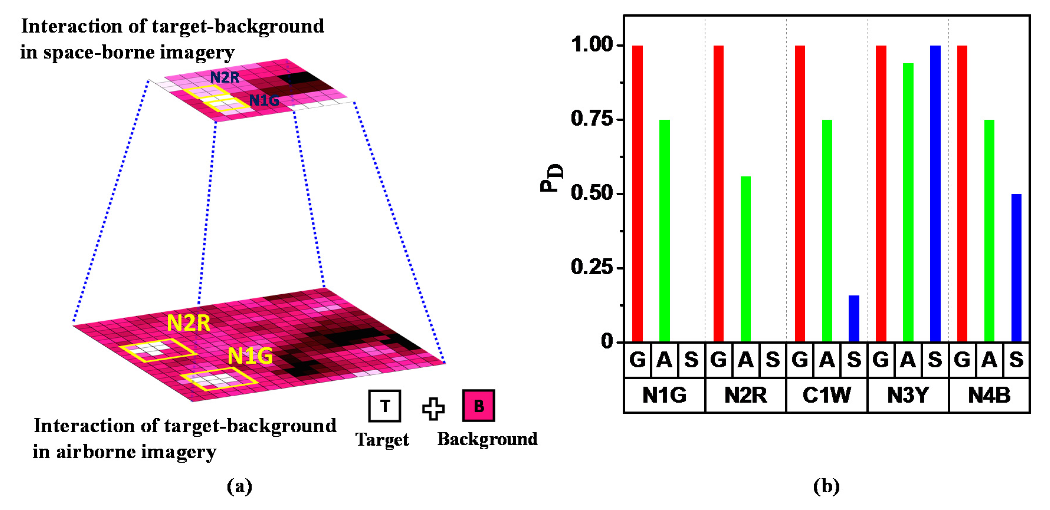
4.2. Target–Background Interaction—Role of Context

To test the impact of contextual background–target spectral interactions on the repeatability of the target detections, we placed targets of identical material in different colors on different backgrounds. Considering the background–target spectral interactions, the detection of identical materials on identical background vary from being systematic and successful to random and fail. With marginal to moderate variations in the false alarm rate (P_FA), our results suggest unambiguous target detection of identical materials on an identical background in both the airborne and space-borne imagery (see Figure 20). Compared to the case of identical materials on identical background, detection rates of identical material targets positioned on different backgrounds vary mainly on the local contrast between target material and background. Accordingly, the detection rates vary from being chance matching to consistent detection. A similar observation has been reported by [6], confirming the substantial effect of scene parameters on the target detection accuracy. In addition, we find that the potential of background interference for altering the detection scores depends substantially on the source of reference target spectra and the detection algorithm.

The variability in the detection rate of identical materials poses a plausible question: How do we standardize the detection rate and ensure detection reproducibility under different environmental, background, and other geometrical factors? The inconsistency in the detection performance needs to be addressed from an algorithmic design perspective, modeling and incorporating the source of uncertainties in the reference target reflectance spectra as observed by different sensors. One of the primary causes for the different detection rates is the non-linearity in the contextual background reflectance recorded by sensors at different platforms, as shown in Figure 21a. Modeling the reference target spectra with possible background mixtures and developing contextual-background sensitive algorithms may enhance target detections across platforms and sensors. Overall, we observe that targets placed on a comparatively reflective local background are detected with lower false alarms $\left(P_{FA}~{10}^{-4}\right)$ by all the algorithms. Although a detailed analysis of the role of background is not in the purview of this paper, our results support the theoretical perspectives of different target-background outlined by [37], and we suggest maintaining a balance between model sophistication and its real-time applicability.

4.3. Detection Algorithms and Their Functional Categorization

Apart from the spectral-geometrical-imaging platform dynamics of the target materials, detection algorithms play a key role in recognizing and identifying material targets. Given the acquisition of appropriate spectral imagery and meeting the minimum dimension of the target material, the detection algorithm employed determines the possibility and quality of target detections. For the given target reference spectra, the functional characterization expected from a potential detection algorithm is the ability to deal with target–background interactions and spectral pattern discrimination in imagery. Based on the functional characteristics, we used three types of detection algorithms, belonging to categories of geometric approach, spectral matching, and background characterization. Target detection of materials in the airborne imagery, with target reference spectra extracted from the same imagery, is accurate and complete (at $P_D$ = 75%) by most of the detection algorithms and the material targets. However, major performance missings of the detection algorithms can be attributed to the sensitivity to backgrounds. The detection rate of an identical material target positioned on two different backgrounds varied substantially by the detection algorithm. Among the spectral matching based detectors, CEM consistently detected material targets across the source of reference target spectra and imagery platform. Yet, the average number of false alarms is ~50, predominantly in the urban areas (see Figure 5), which may not meet the practical target detection purposes. The performance of subspace-based detectors is determined by the quality of extracted endmembers, which in turn depends upon the endmember extraction algorithm used. For example, OSP and TCIMF yielded the lowest false alarms for some materials ($P_{FA}~{10}^{-5}$ for N1G and C1W), but high false alarms for other materials (N4B, N3Y with $P_{FA}~{10}^{-2}\mathrm{to}{10}^{-4}$) (see results in Section 3.1.1). However, for the two similar materials placed on a different contextual background, the detection rate varied drastically between the spectral and subspace-based detectors. For example, for the MF the difference in the detection rate between N4B and N1G is ~20 times; whereas, for ACE, it is about 10,000 times.

The adaptability ofthe sub-pixel detection algorithms, such as CEM, TCIMF, ACE, and OSP, for the detection of engineered materials from space-borne imagery is fraught with a large number of false alarms. While the pixels of target materials are detected, the number of false alarms outweighs the detection rate $P_D$ at 75%. For instance, when the $P_D$ is 75, CEM yielded 3260 false alarms for the detection of the N1G from the space-borne imagery. In addition, the effect of target–background interaction(due to mixed pixels) on algorithms’ performance seems pronounced in space-borne imagery (Figure 7). However, when the confidence of the detection rate $P_D$ is reduced to 50%, the results from the space-borne imagery (Sentinel-2 at 10 m resolution) are consistent, indicating the potential utility of space-borne imagery for target reconnaissance. We find that the state of the art target detectors needs substantial refinements for target detection problems. A couple of studies suggest the use of local mean and covariance estimation, and quantification of interaction effects for improved detection [4,36]. Algorithms with adaptive target–background signal modeling with incorporations of non-linear signal mixing models for sub-pixel/mixed pixel targets can provide better results compared to the traditional statistical detectors.

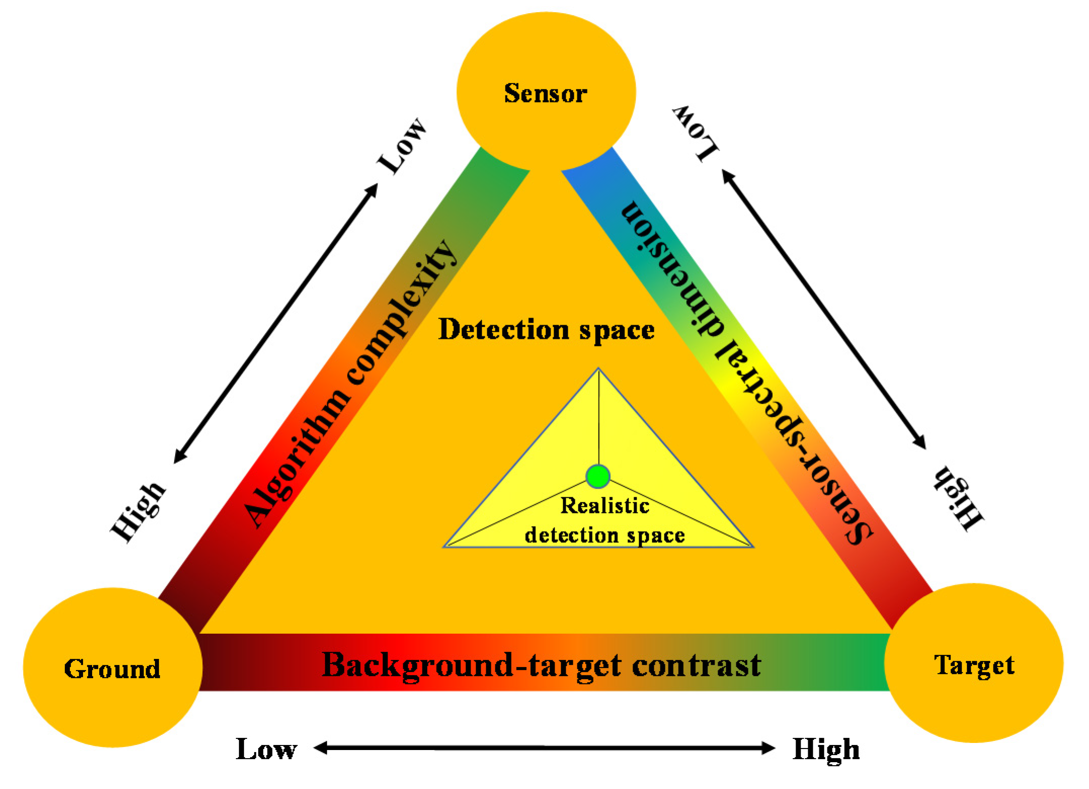
4.4. Key Elements of Influence in Target Detection

Based on our analyses of the extensive target detections observed under different combinations of background, material, and detection algorithms, we present an empirical estimation of the relative contributions of the three key elements of a remote sensing-based target detection system—ground (including local background), sensor (spectral properties), and target (types and positioning) as vertices of an isosceles triangle. As illustrated in Figure 22, the target detection space represents the possibility of detecting material targets under the full detection possibility (area of the triangle) considering the possible levels of the three key elements. The quality of detections depends upon finding the optimal range in each of the key elements and modeling the appropriate weights. Background contrast (as defined from the target spectral attributes), and sophistication of detection algorithm (ability to localize the target–background spectral attributes) have major contribution compared to the spectral dimensionality of imagery. The spectral features and detection algorithms have equal participation (about 35% each) in the detection as represented by sides of the triangle (Figure 22). The base of the triangle, the target-background, has about 30% contribution in the detection and is a landscape driven parameter, not amenable for prior human intervention. Improvement in the precision and detection scores, representing the height of the triangle, is the sophistication of detection algorithms with reference to optimal spectral dimensionality. A stable target detection system will be the weighted combination of the three key elements and will have its detection scores in the triangle represented by ‘realistic detection space’. Reaching the most optimized combination of the key elements (indicated by the green circular dot) is the theoretical upper limit of the target detection system.

4.5. Experimental Dataset

The multi-source multi-platform dataset for target detection will be a valuable resource for the ongoing efforts on target detection using hyperspectral and multispectral remote sensing data. The high-quality in-situ reference spectral data, acquired both in point and pixel mode, will be helpful to test the nuances of detection related problems and assessment of detection algorithms. Since the present dataset was acquired from an urban neighborhood, the complexity of the imagery would provide a rigorous test to the existing theories about the detection problems. The detection of engineered material at pixel level from satellite data is vital for strategic purposes, and the dataset acquired in this research can be used for validating such endeavor. For all the practical purposes, we propose that the detection metric ($P_D$) of target detectors should be relaxed and re-evaluated according to the imaging complexity of the scene. Target detection can be undertaken in both the reflectance and radiance modes. However, for the present work, we have only tested the detection performance in the reflectance domain. Radiance domain target detection will be pursued as future work. The experimental dataset used in this study will be made available on an appropriate freely accessible public platform.

5. Conclusions

Detection of a specific material of interest/target has been one of the promising applications of remote sensing. Contributing to the public availability of benchmark and comprehensive datasets for target detection studies, we have acquired a benchmark multi-platform remote sensing dataset for exploring the various perspectives target detections and algorithms development and evaluation. We have carried out experiments on target detections as a function of sensor, platform, target–background, and the source of reference target spectra. We observe unambiguous detection of targets in the airborne imagery. The false alarm rate is substantially low if the probability of detection (P_D) is reduced to 75%.The continuity and the quality of target detections are found to be influenced by the source of reference target spectra. While the target–background interaction is one of the key components determining the quality of detection, it is not a decisive constraint on the overall detection of targets. Target detection results from the ground-level hyperspectral imagery based target reference spectra are at par with point-based in-situ target reference spectra. The ground-based hyperspectral imaging sensor is a viable source for rapid acquisition of target reference spectra. A non-imaging spectroradiometer generated in situ reference spectrum may not conform to the landscape area element based target pixel spectrum in spectralimagery. The continuity of target detections from the ground to space, though with different proportions of false positives, suggests the viability of satellite imagery-based target detection. However, further experiments are required to generalize this observation.

Notwithstanding the quality spectral data sources, detection algorithm determines the quality of target detections. The false positives rate is substantial in most of the detection algorithms evaluated, calling for the development of multi-resolution spectral dimensionality invariant target detection algorithms. Since remote sensing-based target detection finds applications in various strategic and civilian applications, the dataset generated in our experiment will help the research community to validate detection algorithms.

References

1. Baldridge, A.M.; Hook, S.J.; Grove, C.I.; Rivera, G. The ASTER spectral library version 2.0. Remote Sens. Environ. 2009, 113, 711–715. [Google Scholar] [CrossRef]
2. Kokaly, R.F.; Clark, R.N.; Swayze, G.A.; Livo, K.E.; Hoefen, T.M.; Pearson, N.C.; Wise, R.A.; Benzel, W.M.; Lowers, H.A.; Driscoll, R.L.; et al. USGS Spectral Library Version 7. Geol. Surv. Data Ser. 2017. [Google Scholar] [CrossRef]
3. Meerdink, S.K.; Hook, S.J.; Roberts, D.A.; Abbott, E.A. The ECOSTRESS spectral library version 1.0. Remote Sens. Environ. 2019, 230, 111196. [Google Scholar] [CrossRef]
4. Cohen, Y.; August, Y.; Blumberg, D.G.; Rotman, S.R. Evaluating subpixel target detection algorithms in hyperspectral imagery. J. Electr. Comput. Eng. 2012. [Google Scholar] [CrossRef]
5. Archer, C.; Morgenstern, J.; Musallam, R.N. Improved target recognition with live atmospheric correction. In Algorithms and Technologies for Multispectral, Hyperspectral, and Ultraspectral ImageryXIX; International Society for Optics and Photonics: Baltimore, MD, USA, 18 May 2013; Volume 8743, p. 87430. [Google Scholar]
6. Yadav, D.; Arora, M.K.; Tiwari, K.C.; Ghosh, J.K. Parameters affecting target detection in VNIR and SWIR range. Egypt. J. Remote Sens. Space Sci. 2018, 21, 325–333. [Google Scholar] [CrossRef]
7. Cheng, G.; Han, J. A survey on object detection in optical remote sensing images. ISPRS J. Photogramm. Remote Sens. 2016, 117, 11–28. [Google Scholar] [CrossRef] [Green Version]
8. Kanjir, U.; Greidanus, H.; Oštir, K. Vessel detection and classification from spaceborne optical images: A literature survey. Remote Sens. Environ. 2018, 207, 1–26. [Google Scholar] [CrossRef] [PubMed]
9. Briottet, X.; Boucher, Y.; Dimmeler, A.; Malaplate, A.; Cini, A.; Diani, M.; Bekman, H.H.P.T.; Schwering, P.; Skauli, T.; Kasen, I.; et al. Military applications of hyperspectral imagery. In Targets and Backgrounds XII: Characterization and Representation; International Society for Optics and Photonics: Orlando (Kissimmee), FL, USA, 4 May 2006; Volume 6239, p. 62390. [Google Scholar]
10. Yuen, P.W.; Richardson, M. An introduction to hyperspectral imaging and its application for security, surveillance and target acquisition. Imaging Sci. J. 2010, 58, 241–253. [Google Scholar] [CrossRef]
11. Molan, Y.E.; Refahi, D.; Tarashti, A.H. Mineral mapping in the Maherabad area, eastern Iran, using the HyMap remote sensing data. Int. J. Appl. Earth Obs. Geoinf. 2014, 27, 117–127. [Google Scholar] [CrossRef]
12. Hou, Y.; Zhang, Y.; Yao, L.; Liu, X.; Wang, F. Mineral target detection based on MSCPE_BSE in hyperspectral image. In Proceedings of the 2016 IEEE InternationalGeoscience and Remote Sensing Symposium (IGARSS), Beijing, China, 10–15 July 2016; pp. 1614–1617. [Google Scholar]
13. Dos Reis Salles, R.; Souza Filho, C.R.; Cudahy, T.; Vicente, L.E.; Monteiro, L.V.S. Hyperspectral remote sensing applied to uranium exploration: A case study at the Mary Kathleen metamorphic-hydrothermal U-REE deposit, NW, Queensland, Australia. J. Geochem. Explor. 2017, 179, 36–50. [Google Scholar] [CrossRef]
14. Snyder, D.; Kerekes, J.; Fairweather, I.; Crabtree, R.; Shive, J.; Hager, S. Development of a web-based application to evaluate target finding algorithms. In Proceedings of the IGARSS 2008-IEEE International Geoscience and Remote Sensing Symposium, Boston, MA, USA, 7–11 July 2008; Volume 2, p. 915. [Google Scholar]
15. Manolakis, D.; Marden, D.; Shaw, G.A. Hyperspectral image processing for automatic target detection applications. Linc. Lab. J. 2003, 14, 79–116. [Google Scholar]
16. Acito, N.; Matteoli, S.; Rossi, A.; Diani, M.; Corsini, G. Hyperspectral airborne “Viareggio 2013 Trial” data collection for detection algorithm assessment. IEEE J. Sel. Top. Appl. Earth Obs. Remote Sens. 2016, 9, 2365–2376. [Google Scholar] [CrossRef]
17. Hamlin, L.; Green, R.O.; Mouroulis, P.; Eastwood, M.; Wilson, D.; Dudik, M.; Paine, C. Imaging spectrometer science measurements for terrestrial ecology. In Proceedings of the AVIRIS and New Developments. 2011 Aerospace Conference, Big Sky, MT, USA, 5–12 March 2011; pp. 1–7. [Google Scholar]
18. Bhattacharya, B.K.; Green, R.O.; Rao, S.; Saxena, M.; Sharma, S.; Kumar, K.A.; Srinivasulu, P.; Sharma, S.; Dhar, D.; Bandyopadhyay, S.; et al. An overview of AVIRIS-NG airborne hyperspectral science campaign over India. Curr. Sci. 2019, 116, 1082–1088. [Google Scholar] [CrossRef]
19. SVC-Field-Spectroscopy-Guide-Rev-1-2019-10-22.pdf. Available online: https://www.spectravista.com/wp-content/uploads/2019/12/SVC-Field-Spectroscopy-Guide-Rev-1-2019-10-22.pdf (accessed on 19 June 2020).
20. Adler-Golden, S.; Berk, A.; Bernstein, L.S.; Richtsmeier, S.; Acharya, P.K.; Matthew, M.W.; Anderson, G.P.; Allred, C.L.; Jeong, L.S.; Chetwynd, J.H. FLAASH, a MODTRAN4 atmospheric correction package for hyperspectral data retrievals and simulations. In Summaries of the Seventh JPL Airborne Earth Science Workshop; Jet Propulsion Laboratory, California Institute of Technology: Pasadena, CA, USA, 16 January 1998; Volume 1, pp. 9–14. [Google Scholar]
21. Gruninger, J.H.; Ratkowski, A.J.; Hoke, M.L. The Sequential Maximum Angle Convex Cone (SMACC) Endmember Model. In Algorithms and Technologies for Multispectral, Hyperspectral, and Ultraspectral ImageryX; International Society for Optics and Photonics: Orlando, FL, USA, 12 August 2004; Volume 5425. [Google Scholar]
22. Manolakis, D.G.; Lockwood, R.B.; Cooley, T.W. Hyperspectral Imaging Remote Sensing: Physics, Sensors, and Algorithms; Cambridge University Press: Cambridge, UK, 2016. [Google Scholar]
23. Kay, S.M. Fundamentals of Statistical Signal Processing: Detection Theory; Prentice Hall PTR: Upper Saddle River, NJ, USA, 1993; Volume II. [Google Scholar]
24. Kruse, F.A.; Lefkoff, A.B.; Boardman, J.W.; Heidebrecht, K.B.; Shapiro, A.T.; Barloon, P.J.; Goetz, A.F.H. The spectral image processing system (SIPS)—Interactive visualization and analysis of imaging spectrometer data. Remote Sens. Environ. 1993, 44, 145–163. [Google Scholar] [CrossRef]
25. Manolakis, D. Detection algorithms for hyperspectral imaging applications: A signal processing perspective. In Proceedings of the 2003 IEEE Workshop onAdvances in Techniques for Analysis of Remotely Sensed Data, Greenbelt, MD, USA, 27–28 October 2003; pp. 378–384. [Google Scholar]
26. Chang, C.I. Hyperspectral Imaging: Techniques for Spectral Detection and Classification; Springer Science & Business Media: New York, NY, USA, 2003; Volume 1. [Google Scholar]
27. Scharf, L.L.; McWhorter, L.T. Adaptive matched subspace detectors and adaptive coherence estimators. In Proceedings of the Conference Record of the Thirtieth Asilomar IEEE Conference on Signals, Systems and Computers, Pacific Grove, CA, USA, 3–6 November 1996; pp. 1114–1117. [Google Scholar]
28. Harsanyi, J.C.; Chang, C.I. Hyperspectral image classification and dimensionality reduction: An orthogonal subspace projection approach. IEEE Trans. Geosci. Remote Sens. 1994, 32, 779–785. [Google Scholar] [CrossRef] [Green Version]
29. Ren, H.; Chang, C.I. Target-constrained interference-minimized approach to subpixel target detection for hyperspectral images. Opt. Eng. 2000, 39, 3138–3146. [Google Scholar] [CrossRef]
30. Fawcett, T. An introduction to ROC analysis. Pattern Recognit. Lett. 2006, 27, 861–874. [Google Scholar] [CrossRef]
31. Krawczyk, B. Learning from imbalanced data: Open challenges and future directions. Prog. Artif. Intell. 2016, 5, 221–232. [Google Scholar] [CrossRef] [Green Version]
32. Chang, C.I. An information-theoretic approach to spectral variability, similarity, and discrimination for hyperspectral image analysis. IEEE Trans. Inf. Theory 2000, 46, 1927–1932. [Google Scholar] [CrossRef] [Green Version]
33. Robila, S.A.; Gershman, A. Spectral matching accuracy in processing hyperspectral data. In Proceedings of the IEEE International Symposium on Signals, Circuits and Systems (ISSCS 2005), Iasi, Romania, 14–15 July 2005; Volume 1, pp. 163–166. [Google Scholar]
34. Van der Meer, F. The effectiveness of spectral similarity measures for the analysis of hyperspectral imagery. Int. J. Appl. Earth Obs. Geoinf. 2006, 8, 3–17. [Google Scholar] [CrossRef]
35. Goodenough, A.A.; Brown, S.D. DIRSIG 5: Core design and implementation. In Algorithms and Technologies for Multispectral, Hyperspectral, and Ultraspectral ImageryXVIII; International Society for Optics and Photonics: Baltimore, MD, USA, 2012; Volume 8390, p. 83900. [Google Scholar]
36. Wang, Z.; Xue, J.-H. The matched subspace detector with interaction effects. Pattern Recognit. 2017, 68, 24–37. [Google Scholar] [CrossRef]
37. Matteoli, S.; Diani, M.; Theiler, J. An overview of background modeling for detection of targets and anomalies in hyperspectral remotely sensed imagery. IEEE J. Sel. Top. Appl. Earth Obs. Remote Sens. 2014, 7, 2317–2336. [Google Scholar] [CrossRef]
Figure 1. Conceptual design of the experimental set up used for the acquisition of multi-platform remote sensing data.
Remotesensing 12 02145 g001
Figure 2. (a) True color composite of the AVIRIS-NG hyperspectral imagery with the locations of the artificial targets earmarked; (b) location of targets—N3Y and N4B; (c) location of targets—C1W, N1G, and N2R; (d) ground truth map, and (ef) enlarged view of the ground truth map for different targets. Field photographs (gk) showing the artificial targets placed in the study area for imagery acquisition.
Remotesensing 12 02145 g002
Figure 3. Reference spectral signatures of the artificial target materials acquired from in-situ reflectance measurements.
Remotesensing 12 02145 g003
Figure 4. Methodological framework adopted for the target detection in multi-platform remote sensing imagery.
Remotesensing 12 02145 g004
Figure 5. Target detection performance comparison in airborne imagery for the in-situ target reference spectra. Receiver operation curves (ROC) for the detection from spectral angle mapper (SAM), adaptive cosine estimator (ACE), constrained energy minimization (CEM), and matched filter (MF) for the (a) N1G, (b) N2R, (c) C1W, (d) N3Y, and (e) N4B targets. ROC curves for the detection from orthogonal subspace projection (OSP) and transformed constrained interference minimization filter (TCIMF) for the N1G, N2R, C1W, N3Y, and N4B targets for (fj) 5, (ko) 10, and (pt) 15 background materials.
Remotesensing 12 02145 g005
Figure 6. Target detection score image from (a) airborne imagery using in-situ reference target spectra, and the enlarged detection score footprint for (b) N3Y, (c) N4B, (d) N1G, (e) N2R, and (f) C1W target (In all the target detection score images, a brighter pixel indicates a higher target detection score and thus a higher probability for it to be declared as a target).
Remotesensing 12 02145 g006
Figure 7. Target detection performance comparison from space-borne imagery for the in-situ target reference spectra. ROC curves for the detection from SAM, ACE, CEM, and MF for the (a) N1G, (b) N2R, (c) N3Y, (d) C1W, and (e) N4B targets. ROC curves for the subspace-based detector OSP and TCIMF for the N1G, N2R, N3Y, C1W, and N4B targets for (fj) 5, (ko) 10, and (pt) 15 endmember/background materials.
Remotesensing 12 02145 g007
Figure 8. Target detection score image (a) from space-borne imagery using in-situ target reference spectrum and the enlarged detection score footprint for (b) N3Y, (c) N4B, (d) N1G, (e) N2R, and (f) C1W targets.
Remotesensing 12 02145 g008
Figure 9. Target detection performance comparison in airborne imagery for the terrestrial hyperspectral imager (THI) target reference spectra. ROC curves for the detection from SAM, ACE, CEM, and MF for the (a) N1G, (b) N2R, (c) N3Y, and (d) N4B targets. ROC curves for the subspace-based detector OSP and TCIMF for the N1G, N2R, N3Y, and N4B targets for (eh) 5, (i-l) 10, and (mp) 15 endmember/background materials.
Remotesensing 12 02145 g009
Figure 10. Target detection score image from (a) airborne imagery using THI target reference spectrum and the enlarged detection score footprint for (b) N3Y, (c) N4B, (d) N1G, and (e) N2Rtarget.
Remotesensing 12 02145 g010
Figure 11. Target detection performance comparison in space-borne imagery for the THI target reference spectra. ROC curves for the detection from SAM, ACE, CEM, and MF for the (a) N1G, (b) N2R, (c) N3Y, and (d) N4B targets. ROC curves for the subspace-based detector OSP and TCIMF for the N1G, N2R, N3Y, C1W, and N4B targets for (eh) 5, (il) 10, and (mp) 15 endmember/background materials.
Remotesensing 12 02145 g011
Figure 12. Target detection score image from (a) space-borne imagery using THI target reference spectra and the enlarged detection score footprint for (b) N3Y, (c) N4B, (d) N1G, and (e) N2R target.
Remotesensing 12 02145 g012
Figure 13. Target detection performance comparison in airborne imagery for the airborne target reference spectra. ROC curves for the detection from SAM, ACE, CEM, and MF for the (a) N1G, (b) N2R, (c) N3Y, (d) C1W, and (e) N4B targets. ROC curves for the subspace-based detector OSP and TCIMF for the N1G, N2R, N3Y, C1W, and N4B targets for (fj) 5, (ko) 10, and (pt) 15 endmember/background materials.
Remotesensing 12 02145 g013
Figure 14. Target detection score image from (a) airborne imagery using airborne target reference spectrum and the enlarged detection score footprint for (b) N3Y, (c) N4B, (d) N1G, (e) N2R, and (f) C1W target.
Remotesensing 12 02145 g014
Figure 15. Target detection performance comparison in space-borne imagery for the airborne target reference spectra. ROC curves for the detection from SAM, ACE, CEM, and MF for the (a) N1G, (b) N2R, (c) N3Y, (d) C1W, and (e) N4B targets. ROC curves for the subspace-based detector OSP and TCIMF for the N1G, N2R, N3Y, C1W, and N4B targets for (fj) 5, (ko) 10, and (pt) 15 endmember/background materials.
Remotesensing 12 02145 g015
Figure 16. Target detection score image from (a) space-borne imagery using airborne target reference spectrum and the enlarged detection score footprint for (b) N3Y, (c) N4B, (d) N1G, (e) N2R, and (f) C1W target.
Remotesensing 12 02145 g016
Figure 17. Target detection performance comparison in space-borne imagery for the airborne target reference spectra. ROC curves for the detection from SAM, ACE, CEM, and MF for the (a) N1G, (b) N2R, (c) N3Y, (d) C1W, and (e) N4B targets. ROC curves for the subspace-based detector OSP and TCIMF for the N1G, N2R, N3Y, C1W, and N4B targets for (fj) 5, (ko) 10, and (pt) 15 endmember/background materials.
Remotesensing 12 02145 g017
Figure 18. Target detection score image from (a) space-borne imagery using space-borne target reference spectrum and the enlarged detection score footprint for (b) N3Y, (c) N4B, (d) N1G, (e) N2R, and (f) C1W target.
Remotesensing 12 02145 g018
Figure 19. Spectral comparison of the reference target spectra with the corresponding image target spectra for: (I) in-situ measurements of (a,f) N1G, (b,g) N2R, (c,h) C1W, (d,i) N3Y, and (e,j) N4B compared to airborne and space-borne image spectra respectively; (II) THI measurements of (a,e) N1G, (b,f) N2R,(c,g) N3Y, and (d,h) N4B compared to airborne and space-borne image spectra respectively;and (III) airborne measurements of (a) N1G, (b) N2R, (c) C1W, (d) N3Y, and (e) N4B compared to space-borne image spectra.
Remotesensing 12 02145 g019
Figure 20. False alarms at different levels of P D for (I) identical target material (N1G and N2R) in the same context (vegetative) for the (a) best case, and (b) worst-case detection performance; (II) identical target material (N1G and N3Y) in a different context (vegetation and soil respectively) for (c) best case, and (d) worst-case detection performance.
Remotesensing 12 02145 g020
Figure 21. (a) Visualization of the non-linear interaction of background signal with the target spectrum for the N2R and N1G targets, and (b) best case target detection continuum results of detection performance across imagery from all the platforms (G-ground, A-airborne, S-space-borne) for all the targets used in at a false alarm rate of 10−3 for the in-situ target reference spectra.
Remotesensing 12 02145 g021
Figure 22. Various elements of a target detection system and their mutual correlation in the detection space.
Remotesensing 12 02145 g022