Data Reconstruction for Remotely Sensed Chlorophyll-a Concentration in the Ross Sea Using Ensemble-Based Machine Learning


1
Department of Oceanography, Pusan National University, Geumjeong-Gu, Busan 46241, Korea
2
Korea Polar Research Institute, Incheon 21990, Korea
*
Author to whom correspondence should be addressed.
Remote Sens. 2020, 12(11), 1898; https://doi.org/10.3390/rs12111898
Submission received: 28 April 2020
/
Revised: 10 June 2020
/
Accepted: 10 June 2020
/
Published: 11 June 2020
(This article belongs to the Section Ocean Remote Sensing)
Abstract
:Polar regions are too harsh to be continuously observed using ocean color (OC) sensors because of various limitations due to low solar elevations, ice effects, peculiar phytoplankton photosynthetic parameters, optical complexity of seawater and persistence of clouds and fog. Therefore, the OC data undergo a quality-control process, eventually accompanied by considerable data loss. We attempted to reconstruct these missing values for chlorophyll-a concentration (CHL) data using a machine-learning technique based on multiple datasets (satellite and reanalysis datasets) in the Ross Sea, Antarctica. This technique—based on an ensemble tree called random forest (RF)—was used for the reconstruction. The performance of the RF model was robust, and the reconstructed CHL data were consistent with satellite measurements. The reconstructed CHL data allowed a high intrinsic resolution of OC to be used without specific techniques (e.g., spatial average). Therefore, we believe that it is possible to study multiple characteristics of phytoplankton dynamics more quantitatively, such as bloom initiation/termination timings and peaks, as well as the variability in time scales of phytoplankton growth. In addition, because the reconstructed CHL showed relatively higher accuracy than satellite observations compared with the in situ data, our product may enable more accurate planktonic research.
1. Introduction
Ocean color (OC) sensors are critical resources for ocean biology, biogeochemistry and climatic research [1,2]. The substantial space and time coverages of the sensors have made these sensor indispensable to the studies on the oceanographic dynamics of marine ecosystems [3]. Furthermore, the OC sensors have been widely used to study various phenomena, such as harmful algal blooms [4], maritime disasters [5,6,7], coral reefs [8] and sediment plumes [9]. In particular, because the chlorophyll-a concentration (CHL, mg m−3) in a euphotic zone, which is a representative product derived from the OC measurements, is strongly related to phytoplankton abundance, CHL has a vital role in elucidating the pattern of the phytoplankton growth [10], primary production [11] and global carbon cycle through remotely measured carbon dioxide pressure [12,13] over the global oceans.
High-resolution (from hundreds of meters to thousands of kilometers) OC sensors have been monitoring our planet almost every day since the late 1990s. The quantity of data has been gradually increasing over the last two decades. Additionally, because the efforts of many researchers have greatly improved the quality of this enormous dataset, its potential availability has grown dramatically in recent years. Nevertheless, in the polar regions, the continuous use of OC remote sensing has several limitations due to low solar elevations, ice effects [14], peculiar phytoplankton photosynthetic parameters [15], optical complexity of seawater [16] and persistence of clouds and fog [17]. For these reasons, since the valid values rarely remain, there are practical constraints to polar studies based on these OC measurements.
The polar regions are now experiencing various environmental changes with respect to current and projected climate change, such as melting snow, glaciers and sea ice, permafrost thaw, ocean acidification and changes in hydrology and ecosystems. Some of these result in positive feedback loops that exacerbate the problem. Despite these implications, it is difficult to detect climate-induced changes due to unsecured data quantity and quality. In particular, to understand long-term variability in marine ecosystems associated with climate change, it is vital to consider the error of generalization. In other words, it should not be presumed that the interpretation based on insufficient observations caused by many gaps is similar to the general ecological characteristics of the region. Conventionally, many researchers have used OC data using spatial or temporal (monthly or annually) means to account for the considerable gaps in data. This approach has not taken full advantage of the native resolution of the OC and also suffers from the error of generalization that misrepresents the characteristics of a confined area as those of the entire region.
In the past decade, various efforts have been made to fill these gaps in the OC data to avoid faults of more sophisticated and efficient techniques, such as data interpolating empirical orthogonal functions (DINEOF) [18]. Recently, some artificial intelligence (AI)-based algorithms have been applied to recover the gap data [17,19,20,21]. Jouini et al. [19] reconstructed the CHL in the western sector of the North Atlantic via sea surface temperature (SST) and sea surface height (SSH) using a classification technique called the self-organizing map. They showed that even under 100% cloud cover, the CHL values could be reconstructed at scales larger than 10 km well. Krasnopolsky et al. [20] also applied an AI-based technique to reconstruct the gaps in OC data on a global scale. The reconstruction was based on the physical variables derived from satellite measurements such as SST, SSH and sea surface salinity (SSS) and Argo in situ data. They noted that the application of their approach could provide an accurate, computationally cheap method for filling spatial and temporal gaps in the satellite observations. Chen et al. [21] reconstructed CHL data through an ensemble-based approach (random forest, RF) using wavelength-based predictors. They showed a significant improvement in OC gap recovery of more than 300% over the regions of the Yellow Sea and the East China Sea and the estimated CHL has a quality similar to that of the standard satellite-derived CHL. However, all previous studies have been conducted in non-polar regions, except that of Park et al. [17] (hereafter P2019). P2019 applied a method of reconstructing the missing values on the satellite-derived CHL data in polar regions. They attempted to predict the CHL for the pixels with missing values using ensemble machine-learning-based models with the satellite data of other factors such as sea ice concentration (SIC) and SST and reanalysis data generated by combining observation data and numerical model output. Although the results were robust, their reconstruction had some limitations: (1) The spatial coverage of their reconstruction was too small. Cape Hallett, their study area, is a region without distinct ecological properties (i.e., phytoplankton bloom) in the Ross Sea. Most phytoplankton blooms are concentrated in the western and southern Ross Sea [10]; (2) Because their reconstruction was primarily focused on high model performance, they constrained the span of reconstructed CHL data to 0–3.77 mg m−3. They set a range of reconstructions based only on model performance without any consideration of whether there was a CHL of more than 3.77 mg m−3 in the region. This limitation may result in a significant error in the reconstruction at the CHL values higher than the upper limit value; (3) Their reconstruction is limited to only the open water areas bordered by 15% SIC, which are subject to marginal ice edges. In the current study, such restrictions were redefined with different criteria, and detailed explanations are given in Section 3.1.
Consequently, we produced the gapless CHL dataset using a novel reconstruction model called RF, which is a kind of machine-learning-based ensemble tree algorithm. This work fundamentally follows the concept suggested by P2019, but it does include some critical solutions to the issues that they have, such as the small spatial scale, narrow scope of the reconstructed CHL range and area restricted to the ice-free ocean (<15% ice concentration). This product covers a spatially large scale that includes the Ross Sea shelf region (79–65° S and 140° E–140° W) and has a broader CHL range from 0 to 50 mg m−3 compared with that of P2019. Furthermore, the areas with up to 60% ice concentration that likely to be observable with OC sensor were considered. For better reconstruction model performance, the unnatural data that could interfere with the model development were detected and removed using the normalized median test method (Section 3.1 and Section 4.1) and some procedures such as data transformation (Section 3.2) and model optimization (Section 3.3) were performed. Then, we evaluated the model performance using several evaluation indices (Section 3.4 and Section 4.2). In addition, the model was adjusted by introducing an oversampling technique to solve the low accuracy issue in the minority target class (Section 4.3), and the final evaluation was performed (Section 4.4 and Section 4.5). In Section 3.5 and Section 4.6, the variable importance and partial dependence plot that reflect the contribution of the predictive variables to the model development were described. Finally, the challenges that remained despite our efforts and the benefits of the CHL product retrieved from this research were discussed in Section 5.
2. Data
For the reconstruction model development focused on the Ross Sea, the information on the input (predictive) and the target (responsive) variables are listed in Table 1. The variable selection was established based on the relationship between the physical oceanographical factors from the local to global scale and phytoplanktonic dynamics in the Ross Sea region, revealed by many previous studies [22,23,24,25,26,27,28,29,30,31,32,33,34,35,36], as suggested in P2019 (see Section 4.1 in P2019).
2.1. Satellite and Reanalysis Datasets
The CHL data were used as the target data to be reconstructed and the climatology of the CHL during summertime (November 1 to March 31) was used as a predictor of the reconstruction model. The CHL data were a Level-3 9 km standard mapped image produced by the visible infrared imaging radiometer suite (VIIRS) mounted on the suomi national polar-orbiting partnership and was obtained from the NASA ocean color website (https://oceancolor.gsfc.nasa.gov/).
Because these data date back to late 2012, this study is limited to a total of six spring and summer periods from 2012/2013 to 2017/2018. For the SST data, we used the multiscale ultra-high resolution sea surface temperature (MURSST) data provided by the Jet Propulsion Laboratory (https://www.mur.jpl.noaa.gov), which are available from 2002 to the present. Some other relevant satellite-based data used in this study are the SIC data. These data were not used directly for the model development but used as a reference for masking. The SIC data were derived from the University of Bremen’s ARTIST (Arctic radiation and turbulence interaction study) sea ice (ASI) algorithm [37]. This algorithm has a resolution of approximately 10 km on a polar stereographic grid using the full resolution of the advanced microwave scanning radiometer 2. These data are available at https://seaice.uni-bremen.de/amsr2/index.html.
2.2. Other Input Variables
Variables such as the 2-meter atmospheric temperature (T2M), photosynthetically available radiation (PAR), 10-meter zonal (U10) and meridional (V10) winds that could not be obtained from the satellite observations were derived from the ERA-interim reanalysis data provided by the European Center for Medium-Range Weather Forecasts (https://www.ecmwf.int). Although the PAR data can be obtained from the OC sensor, these data also have many gaps. Due to the characteristics of the model developed here, the data cannot be reconstructed in pixels where even one gap exists in the input data. Therefore, the ERA-interim dataset with no gaps was used for the PAR data. In addition, ocean floor depth (DEP) data, used as a predictor (input variable), were provided by the general bathymetric chart of the ocean, and have a spatial resolution of approximately 30 arc-seconds (https://www.gebco.net). These digital bathymetry data have higher accuracy in combination with the acoustic in situ measurements and satellite-based gravity data. The ocean floor depth, the longitude (LON), latitude (LAT) and days of the year (DOY) are additionally used as predictors that do not control the CHL variation directly. These factors were used to illustrate the climatology of the CHL over the Ross Sea and to consider the remaining factors for CHL changes that the environmental predictor selected here (SST, T2M, U10 and V10) cannot explain.
2.3. In Situ Measurements
Observing polar regions is considerably difficult because access is limited due to the harsh marine environment (e. g., the presence of sea ice). Although this type of study requires a large amount of actual data to evaluate the acceptability of the reconstruction results, it is practically impossible to secure enough spatially uniform data, especially throughout our research area, the Ross Sea (Figure 1). Therefore, we used the in situ measurements obtained within the Ross Sea that are publicly available. The first measurement was conducted onboard the RV/IB Nathaniel B. Palmer from February 12 to March 18, 2013 (NBP1302). The data were extracted from the data files provided by Smith and Kaufman [38]. Second, the CHL analyzed in uncontaminated near-surface (3 to 7 m) water samples obtained from the “pump-underway ship intake” system during the same cruise was used (NBP1302U). The dataset was obtained from the Biologic & Chemical Oceanography Data Management Office website https://www.bco-dmo.org. Another survey was then conducted onboard the same ship from December 31, 2017, to February 19, 2018 (NBP1712), which was obtained from the U.S. Antarctic Program Data Center [39]. Of the collected CHL data from all the stations of the NBP1302, NBP1302U and NBP1712 surveys, we did not consider the information at the stations where no CHL observations were performed, that have more than 60% ice concentration or where no data above a 10-meter depth were obtained. In addition, the mean values in the 5 × 5 pixels centered on the pixel with the location of the in situ measurement on the standard satellite-based and reconstructed CHL datasets were matched with the satellite data to minimize the uncertainties that contribute to the temporal and spatial mismatch between the in situ observations and mapped CHL datasets. Only if the number of valid pixels in the 5 × 5 pixels was ≥ 10%, the extracted data were used together with the field measurements in the model development. As such, 164 samples (62 stations from NBP1302, 64 stations from NBP1302U and 38 stations from NBP1712) were selected for the comparison with both the standard satellite-derived and the reconstructed CHL dataset.
3. Procedure and Approaches
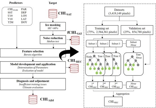
This section first presents an illustration of the workflow of our study (Figure 2). Several methods and model settings used in the process are described in the following subsections.
3.1. Ice Masking and Noise Reduction
Because the OC observation in regions where the sea ice is densely covered is practically impossible, we attempted to mask the CHL data using the SIC. It appears that the OC can be measured in the region with up to 60% SIC on average (not shown). Thus, we decided not to consider the CHL measurements in the areas with a SIC of more than 60% in the model development.
The quality of OC data were improved based on the quality-control flags for various other conditions (e.g., sun zenith angle, cloud, ice cover, atmospheric correction status, land and sun glint). Nevertheless, there were still unusually high or low CHL values that were not consistent with the adjacent measurements, as shown in Figure 3. In these images, these abnormal CHL values are likely attributed to the failure in flagging thin clouds. If these values are used for the reconstruction without any correction, the overall model performance is reduced, and prediction failure could occur. Therefore, we applied a method called "normalized median test" to remove these abnormal CHL values. Conventionally, a simple median filter is often applied before using the CHL data. Still, this method not only results in the coercive deformation of the original data, but also eliminates the boundary values, leading to data loss. However, the normalized median test used here is a way to minimize such deformation and loss.
The initial version, a simple median test, was presented by Westerweel [40] and developed to detect outliers in particle image velocimetry data. This version was improved by Westerweel and Scarano [41] by normalizing the median residual to make it more robust, and we applied this improved method to remove the unnatural values on the gridded CHL images. The procedure of the method is as follows. First, the size () of the subwindow is set. Based on the value of a specific pixel (i.e., the center of the subwindow), a total of adjacent pixel values are determined (). Next, the median of adjacent values, (excluding ) is calculated. Then, the residual for the median () can be calculated as follows.
This value is used to calculate the median of the and normalize the residual of as follows.
where ε may represent the acceptable fluctuation level due to cross-correlation. Finally, a specific threshold () is applied to the calculated , and we set the target to remove pixels with normalized residual values greater than (). Here, we set , ε = 1 and θ = 1.
3.2. Data Transformation and Feature Selection
One of the crucial factors in machine learning is the imbalance of the target class (the “class” refers to CHL in this study.). The bloom, which is implied by an increase in the CHL, in the Ross Sea is characterized by the plankton assemblage in a restricted space and growth/dissolution for a short time scale. Because of these characteristics, the lower CHL values are found more frequently in typical surface oceans than the higher CHL values associated with bloom. Eventually, the CHL data generally do not show a normal distribution and have positive skewness. If the positively skewed data are used to train the model as is, there is a high probability that the prediction of the minority class (CHL values with low data frequency) will fail. Because the basic concept of machine learning itself is optimized for the data in nature, we transformed the target class into a normal distribution that usually appears in natural data on logarithmic scales [3].
When the data transformations were completed, the Boruta algorithm [42], a variable selection technique based on the RF, was used to test how efficiently the selected predictors worked for model development. As such, it was found that the selected variables play a significant role, and we attempted to develop a RF model to reconstruct the CHL data from 2012/2013 to the 2017/2018 summer seasons in the Ross Sea.
3.3. Machine-learning Model
To reconstruct the CHL data, we used the RF model, a type of ensemble learning method for classification and regression analysis and output classifications or average predictions from multiple decision trees constructed during the training process [43]. In general, in order to enable the randomness and independence of each tree, the RF model randomly collects subset samples (by allowing duplicates) through a bootstrap aggregation technique that can improve the stability and accuracy of model performance. The method reduces the variance in the iterative results of the model and can avoid overfitting, causing little difference in performance between the training and test datasets. In addition, the bagging techniques are known to be appropriate for the data containing noise, such as the CHL dataset. The features (input variables) used for node division are limited to ensure diversity between each tree constituting the RF. That is, if all the features are selected when constructing the trees, there will be little difference between the trees. A rule of thumb is that the RF model sets the square root of the total number of features as the parameter on the maximum feature number to produce the best results. Eventually, for the feature selected at each node, the node is divided into two child nodes based on the optimal partitioning condition (i.e., a small mean squared error, MSE), and a leaf node is calculated. Then, finally, the results produced by each tree are ensembled on average to draw a conclusion.
Several parameters must be considered when implementing an RF model that can best fit the target data through a given predictor. The first parameter is the number of features (Mtry). As described above, the Mtry that is generally optimized in the RF model is the square root of the entire feature number; that is, because the total Mtry in this study is 10, Mtry was set to 3. Another vital parameter to consider is the number of single decision trees (Ntree) to use in implementing the ensemble. A high value of Ntree can produce more accurate results, but if it is too high, the computation efficiency will be reduced considerably. Therefore, a balance between accuracy and computational efficiency is required. Through trial and error, the value of Ntree was set to 60 and Mtry was set according to the convention (Mtry =). The two parameters mentioned above showed the most sensitively towards the data given in this study, and the minimum number of samples required to split an internal node and to be at a leaf node were applied as 2 and 1, respectively.
3.4. Model Evaluation Metrics
Various statistical metrics were used to evaluate model performance. It is expected that a more detailed evaluation is possible through these various metrics, and the metrics used are R2, MSE, root mean squared error (RMSE), mean absolute error (MAE), relative RMSE (RRMSE) and root mean absolute error (RMAE). Furthermore, to highlight cross-sensor agreement and bias, an unbiased percent difference (UPD) and mean relative difference (MRD) can be defined as follows [21,44,45].
3.5. Contribution of Predictive Variable for Reconstruction
Decision tree-based algorithms such as RF can measure the variable importance (VI) of features used in model development. The VI could be measured by testing how much the node reduces impurity on average [43]. The VI is calculated as the average of the weights, and the weight of each node is equal to the number of training samples associated with it. After training, this score is calculated for each feature, and the result is normalized so that the total sum of importance is 1. This characteristic makes it possible to infer how a feature causes a class change.
In addition, we used the partial dependence plot (PDP) to confirm how a change in the feature (i.e., predictor) in the trained model ultimately contributed to predicting the target. Moreover, through the PDP, we thought that the PDP could show the sensitivity of the developed model toward the input variables. The PDP is one of the ways to interpret the trained model, allowing the identification of linear, monotonic or more complex relationships between predictors and targets. represent the features in the model (p = 10 in this study).
When splitting x into the set of selected and its complement (), the PDP of the response variable for is defined as
where is the marginal probability density of . can be calculated.
Equation (5) can be estimated from the training data as follows:
where are the values of that occur in the training samples. That is, the effect of all other predictors in the model is averaged. For details, refer to Friedman [46].
4. Results
4.1. Data Filtering for Model Training
The CHL data for model training were reorganized through ice masking and filtering using the normalized median test, as mentioned earlier. As such, there were significant adjustments compared with the CHLSAT data (Figure 4 and Table 2).
The CHLSAT data were mostly concentrated (about 99.99% or more) at a value of less than 10 mg m−3, and the data quantity gradually decreased as the CHL value increased. The values masked by SIC were mostly removed in the range below 10 mg m−3, except that 3 pixels were eliminated in the field 40 mg m−3≤ CHL <50 mg m−3. The mean ± standard deviation of the removed values was approximately 0.20 ± 0.32 mg m−3; these values were mostly found in the range lower than 1 mg m−3. The pixels removed by the normalized median test were composed of those with concentration > 40 mg m−3 and especially the CHLSAT values greater than 50 mg m−3 were completely removed. As a result, this may mean that most CHLSAT values above 40 mg m−3 can be considered as outliers during the normalized median test. Among the in situ measurements (N = 6086) of surface (<10-m depth) CHL during consecutive summer seasons from 1993 to 2012 in the Southern Ocean obtained from the SeaWiFs bio-optical archive and storage system, only one measurement of more than 40 mg m−3 was present (not shown). This high CHL measurement was observed in the Antarctic peninsula coastal region; most of the measurements in the Ross Sea were below 30 mg m−3. Such results may be evidence that the masking and filtering we performed in this study are efficient. Finally, the filtered CHLSAT (fCHLSAT) data were used for machine-learning training to build the reconstructed CHL (CHLREC) data and the total number of pixels to be used for training and validation was 3536,976 without the missing values (see Table 2).
4.2. Overall Assessment of the Model Performance for Reconstruction
We developed the RF model that reconstructs the missing values in the fCHLSAT data through the model setup described earlier. The model performance for the training set (N = 2652,818), which accounts for 75% of the total data, has an accuracy with R2 = 0.99, MSE = 0.02 mg m−3, RMSE = 0.14 mg m−3, MAE = 0.03 mg m−3, RRMSE = 8.06%, RMAE = 4.08%, UPD = 3.12% and MRD = 0.17% (Figure 5). The training seems to have been carried out intensively within the 0.1 to 1 mg m−3 CHL range due to the high data frequency of fCHLSAT. The validation set (N = 884,273), which represents 25% of the total data, also showed high accuracy (R2 = 0.95, MSE = 0.08 mg m−3, RMSE = 0.28 mg m−3, MAE = 0.08 mg m−3, RRMSE = 38.06%, RMAE = 10.25%, UPD = 8.07% and MRD = 0.94%.), but it was confirmed that the variance was slightly larger than that in the training set.
Figure 6 shows the data frequency and reconstruction rate of the CHLREC compared with the fCHLSAT data. The maximum reconstruction rate of the CHLREC was up to 40 times at ~0.3 mg m−3, but in specific ranges (vertical gray solid lines). The number of CHLREC data was less than that of fCHLSAT data, indicating the predictive failure due to over- or underestimation. We defined these parts as reconstruction failure ranges and segmented them into S1 (<0.04 mg m−3) which is the part inferred as overestimation, and S3 presumed to be underestimated (>10.59 mg m−3) (S2 can be defined as the range of successful reconstruction). Most reconstruction seems to have occurred in the segment S2, and more detailed analysis was needed to determine what factors caused the reconstruction failures in segments S1 and S3. Aside from the failure in segment S1 with the low CHL, because the CHL in the segment S3 with high CHL has significant implications for environmental analysis, we determined that it is necessary to diagnose and compensate for the failure in this segment in the reconstruction for time-varying analysis.
4.3. Additional Diagnosis and Adjustment of the Model
Figure 7 shows the results of testing how much reconstruction capability the RF model can have in segments S3 and S1. As in the previous process, the data included in the segments were divided into 75% training data (N = 2,652,818) and 25% validation data (N = 884,273) and training and validation were performed for each segment. The black dots are the performance of the RF model for the training data, and the red dots are that for the validation data. The performance of the model trained with the model configurations mentioned earlier (i.e., Ntree = 60, Mtry = 3) for segment S3 (because it may have a higher analytical significance than that in S1) is R2 = 0.89, MSE = 1.34 mg m−3, RMSE = 1.01 mg m−3, MAE = 0.69 mg m−3, RRMSE = 7.37%, RMAE = 5.01%, UPD = 4.44% and MRD = 0.47%, which is significantly lower than the established model performance. As expected, the performance of the RF model for the validation data were also reduced significantly (R2 = 0.65, MSE = 1.50 mg m−3, RMSE = 1.52 mg m−3, MAE = 1.24 mg m−3, RRMSE = 11.07%, RMAE = 9.00%, UPD = 8.10% and MRD = 0.92%). The performance in the segment S1 also declined significantly compared with that of the established model, but the absolute errors such as MSE, RMSE and MAE, were almost zero. This is because S1 is limited to a range of very small CHL values of less than 0.04 mg m−3. Therefore, we eventually concluded that the difference between fCHLSAT and CHLREC in S1 was negligible. Although the underestimation issue in S3 was already included in the results presented in Section 4.2 (Figure 5), it was difficult to recognize such an issue because the data in S2 accounted for more than 99.9% of the total data. That is, if S2 shows 100% accuracy, even if the model fails for S1 and S3, the overall evaluation of the model may show an accuracy of more than 99.9%.
Model failure in S1 and S3 is likely to occur due to the lack of training data, and we performed oversampling for S3 containing less training data to overcome the issue. The easiest way to oversample is to resample the minority class, i.e., to duplicate the entries or manufacture data, which is the same as what was done previously. More duplicates could result in more accuracy, but overfitting is inevitable. Therefore, considering the proper accuracy, overestimation issue and efficient computation time together, we attempted to determine the number of times the minority class cluster must be increased while maintaining efficiency. As such, it was concluded that it is the most efficient to quadruple the data of S3, and the results for the validation set are R2 = 0.98, MSE = 0.48 mg m−3, RMSE = 0.51 mg m−3, MAE = 0.18 mg m−3, RRMSE = 3.68%, RMAE = 1.30%, UPD = 1.14% and MRD = 0.07% (Figure 8). The difference in performances for the training and validation set is small, suggesting that the performance is not overfitted and significant. Consequently, we believe that this diagnostic process shows effective performance under the configuration of the current RF model when at least 10,000 data are obtained.
4.4. Conclusive Evaluation of the Adjusted CHL Reconstruction Outcome
For the final evaluation of the adjusted CHLREC data (hereafter "CHLADJ"), which was achieved through the process of diagnosis and adjustment of the CHLREC data, we tested the spatiotemporal variation in the CHLADJ. (Figure 9). In the CHLADJ scenes for three consecutive days (two cases on 3 January 2014 and one on 22 January 2017), the CHLADJ images depict the continuous blooms well. In particular, in the fCHLSAT image on 2 January 2014, the missing values generated within the high CHL patch close to 10 mg m−3 in the southwest coastal area of Cape Colbeck (refer to the map in Figure 1) are well reconstructed in both the CHLREC and CHLADJ datasets, even on images from 21 to 23 January 2017.
Both the CHLREC and CHLADJ data were then compared to the in situ measurements to determine how close the reconstructed datasets were to satellite observations (Figure 10). First, because the NBP1302 cruise was mostly carried out around the western Ross Sea in February, a high CHL range (about 1 to 5 mg m−3) was captured. On the contrary, the NBP1712 measurement was performed in December, and most of the low CHL values were recorded because, in this period, the bloom was limited in the central Ross Sea [8]. The NBP1302U cruise has stations on both the low –CHL open ocean and the shelf region characterized by high CHL. When compared with the in situ measurements, the fCHLSAT data exhibit R2 = 0.24, MSE = 0.06 mg m−3, RMSE = 0.25 mg m−3 and MAE = 0.31 mg m−3 and the CHLADJ data have R2 = 0.74, MSE = 0.02 mg m−3, RMSE = 0.16 mg m−3 and MAE = 0.36 mg m−3, showing that the satellite observations have a lower correlation with in situ measurements than the reconstructed CHL values. Such features are particularly evident in the R2.
4.5. Comparative Analysis of Temporal Features
In this section, a comparison is performed to confirm the difference between the fCHLSAT and CHLADJ datasets (Figure 11). This comparison is expected to be evidence of the potential availability of the CHLADJ data for climate research using the time–series properties. There is a significant difference in amplitude between the time–series of the two datasets over the entire Ross Sea. In contrast to the time–series of the fCHLSAT, which had large fluctuations, the time–series of the CHLADJ seem to be quite stable. In general, the high fCHLSAT in November is highly associated with seasonal sea ice reduction. The effective observed pixels at this time began to gradually increase, but not significantly enough to have a stable standard deviation from the mean. As such, this instability may result in the overestimation of the spatial average. When the sea ice begins to melt, the ocean–atmosphere thermal interactions allow considerable cloud formation. Consequently, the available pixels were extremely rare, and the usability of the data increased at the same time once the sea ice was sufficiently melted. At this time, the amplitude of fCHLSAT also begins to be significantly reduced and does not show much difference from the CHLADJ.
4.6. Partial Dependence on CHL Reconstruction
In the PDP results, the CHL tends to increase between about 1 and 2 mg m−3 with the CHLCLIM showing the contribution of the highest VI (25.4% ± 11.8%) but remains constant for further CHLCLIM values (Figure 12). The consistency of the PDP for the CHLCLIM within a specific range is likely to be due to incomplete training induced by insufficient data. Therefore, the PDP for the closest CHLCLIM value that was sufficiently trained is maintained. This characteristic is seen in the PDP for almost all predictors except for LAT. This consistency is not a natural state, so it has no specific meaning. The LAT, the predictor with the second-highest VI (13.3% ± 2.7%), shows a high PDP below approximately 74° S and near 68° S. The values may be determined by the average latitude of the continental shelf, open ocean and near the Mertz Glacier Tongue with the relatively high CHL (refer to Figure 1). The DOY has a VI of approximately 13.0% ± 9.6% and has a bimodal distribution with peaks in December and February (the flat parts are excluded from interpretation). This bimodal feature in the Ross Sea has been well presented by Smith et al. [38] and may be related to the December bloom in the central Ross Sea and the February bloom in the western Ross Sea. The leading four predictors, including the LON variable with a VI of 9.0% ± 0.8%, contained climatological components of the Ross Sea CHL rather than directly affecting its changes. The DEP, which is also a predictor associated with the CHL climatology, is not entirely independent of the leading predictors; therefore, this variable has the lowest VI (6.0% ± 0.3%). Nevertheless, the reason for not excluding the DEP is that it was first identified as a valid predictor through the Boruta algorithm [42] mentioned earlier, and it could explain the climatological components that have not been fully explained by the previous four leading predictors. While the five predictive variables mentioned above are responsible for the climatological aspect of the Ross Sea CHL, the VIs of five environmental variables that may cause the anomaly are within 8% each: T2M (7.6% ± 0.5%), PAR (6.9% ± 1.6%), U10 (6.6% ± 5.9%), V10 (6.3% ± 0.2%) and SST (6.2% ± 0.5%). However, these variables have ranges that are too narrow, and there were some differences between the PDPs on the CHLREC and the CHLADJ. Thus, these results were not interpreted in this study. It is a challenge to obtain the PDP results for these variables’ distinctive meanings by analyzing the response of the phytoplankton to the environmental changes based on the various measurements such as in situ, satellite and reanalysis datasets.
5. Discussion and Conclusions
Considering only the density plots and eight model evaluation indices presented in Figure 5, it is evident that, overall, the model performs well. Consistent with the model evaluation approach undertaken here, most previous studies applying machine learning in this field have simply concluded that the model was well implemented based on such single evaluation indicators. In practice, however, the models do not perform well. One of the most unnoticed cavities is a model failure in the range of target values (for prediction or reconstruction) where training data are insufficient. The model evaluation results in this minority classes (S1 and S3 in Figure 6) are not distinctly confirmed in the overall evaluation results (as Figure 5) compared with that of the majority class (S2 in Figure 6). The model failure in the CHL ranges with the low data frequency (S3) was found and then diagnosed (Figure 7). Because the high CHLs have significant implications for the studies on the phytoplankton bloom, this needs to be solved. To avoid this problem and then raise the reconstruction efficiency, in this study, we used a simple oversampling technique to duplicate existing data. The adjusted model was able to achieve significant improvements with the introduction of such a method (Figure 8), and the overall performance of the adjusted model was impressive based on the spatiotemporal continuity of the CHL (Figure 9) and the relatively high similarity with the in situ data compared with the satellite measurements (Figure 10). Nevertheless, further research is still required for two aspects. First, although various oversampling methods exist, such as the synthetic minority oversampling [47] and adaptive synthetic sampling [48] approaches, most techniques that we have tried produced rather poor results because of fake data production and heterogeneous sampling (by random resampling). At least, of the many methods we tried, the duplication-based method was the most effective. However, even with this method, large uncertainties still exist. There is still no guarantee that the CHL will reappear within these limited CHL-values. Therefore, a precise reconstruction is almost impossible for the minority class because the discrete distribution of data can lead to insufficient training. In other words, if a CHL value has never appeared, it cannot be properly reconstructed through the method based on duplication. Additionally, it may not appropriate to create data through simple relations such as least-square regression artificially. Therefore, it is required to be developed or applied an appropriate method to process these discrete data for an optimized reconstruction model. Second, the CHLADJ produced in this study better matched the field observation data than the fCHLSAT in terms of the R2, MSE and RMSE (Figure 10). It may suggest that the CHLADJ is more accurate than the CHLSAT. However, these comparison results shown here are still not absolute evidence for such a suggestion because it was based on still lacking in situ data (N = 164). Moreover, most field observations have been concentrated in the western Ross Sea due to its ecological importance (see Figure 1). This spatial heterogeneity of the in situ data are hardly considered complete evidence of this conclusion.
We believe that these problems can be solved to some extent by extending the data period and collaborating with other researchers. We targeted a single sensor (VIIRS, since 2012) dataset with no further postprocessing to reconstruct the CHL closest to the satellite observations. Nonetheless, if the study period is further extended using multisensor CHL products, such as GlobColor and the Ocean Color Climate Change Initiative, it would enable the acquisition of higher data frequencies for natural high CHL values as well as the usability of more accumulated field observation data.
In the process of using the ensemble-based machine-learning model, the PDP provides a quantitative description of the dependence of predictors on the response of the target variable (Figure 12) [46]. The PDP characterizes the marginal relationship between the predictor variable of interest and the dependent predictor while accounting for the influence of all other predictors. Models are generally accessible in terms of predictive and interpretive powers. While more sophisticated models with high predictive power are hardly interpretative, a regression-based model can interpret intuitively even if their performance is relatively low. Accordingly, the PDP can be applied universally to various models and is one of the attempts to interpret the relationship between the modeled values and the input variables. With this advantage, many studies have used the PDP to explain the relationships between a responsive variable and environmental predictors in the oceanographic fields (e.g., climate-induced local habitat variability of commercial fishes [49], long-term changes in the trophic position of organisms [50] and nitrogen fixation [51]). In this study, we added geographical features into the model development process such as LAT, LON, DOY and DEP, including CHLCLIM, which is hardly a physical factor. These predictors are not factors leading to a specific CHL change but denote the mean state of the CHL distribution in the Ross Sea. They also contain parts that the physical predictors applied here cannot explain. Therefore, it is incorrect to elucidate the CHL changes through these factors. In addition, the PDPs are flat in the parts where the data frequency of the predictor variable is low. The flatness exhibits response to adjacent and sufficiently trained predictors. Then these flat parts must be excluded from the analysis. We expect that this approach will play an essential role in identifying the deterministic relationship between the environmental variables and the variation in the CHL. Moreover, the PDP allows us to investigate the model sensitivity towards the accuracy of the input variables. For example, for T2M, with the highest VI among the environmental factors, if the actual T2M is assumed to be −1.0 ℃ and the observed T2M is one degree Celsius, an error of approximately 0.05 mg m−3 may occur in the CHL value reconstructed in this model. However, if the observed T2M is −3.0 ℃, the difference between the input value (∆T2M = two degrees Celsius) is consistent with in the previous case, but it may not contribute significantly to the change in the CHL. Although the PDP is a useful tool in terms of the environmental interpretation and sensitivity towards input variables mentioned above, it is still necessary to continuously test whether the response suggested by the PDP occurs in nature. We are working on a quantitative and systematic assessment of how useful PDP is for environmental interpretation, as well as a sensitivity evaluation of the input predictors.
Despite some improvements, in the current version, the model performance does indeed show considerable skill in reconstructing the CHL data, and the products are expected to be applied to various studies of phytoplankton dynamics in the Antarctic Ross Sea. For example, quantitative and detailed studies on characteristics of bloom phenology, such as bloom peaks and timings (initiation and termination), could be possible, as well as the variability of multiple time scales of phytoplankton growth (Figure 13). As shown in Figure 13, the time–series of the climatological fCHLSAT and the CHLADJ show similar seasonal variations in the CHL overall in all regions. However, the significant issue is regarding the length of the error bar associated with the amplitude of the annual variation in the CHL. The amount of cloud cover differs every year, and the spatial average is calculated based only on the CHL values of the limited exposed surface layer. In terms of the amplitude of annual variation, the CHLADJ generally seems to have more stable variations compared with that of the fCHLSAT. This stability may be attributed to the actual CHL difference from year-to-year, but the inconsistency of the number of valid pixels each year is likely to be the more critical factor for significant annual variations, on only the remotely-sensed data. Therefore, the analysis using the CHLADJ data could be more beneficial than that with the fCHLSAT or CHLSAT for the annual variation of phytoplankton biomass because the use of satellite measurements without any treatment could lead to a critical misinterpretation of results. In addition, the fCHLSAT, even in climatology, too often has missing values during the austral spring and summer (November to March). In most regions in Figure 13, including November, a complete data absence often occurred. While these data absence makes it difficult to study short-term phytoplankton dynamics practically, the CHLREC permits the examination of the detailed process of variation over each spring and summer. Notably, it is necessary to test whether these predicted CHL variations (especially the period of permanent data missing) are consistent with the actual CHL variations, and such verification can be achieved by securing many in situ measurements.
Author Contributions
Conceptualization, J.P. and Y.-H.J.; methodology, J.P.; validation, J.P. and D.B.; formal analysis, J.P. and D.B.; investigation, J.P. and D.B.; resources, H.-C.K.; data curation, J.P.; writing—original draft preparation, J.P.; writing—review and editing, Y.-H.J. and H.-C.K.; visualization, J.P.; supervision, H.-C.K. and Y.-H.J.; project administration, H.-C.K.; and funding acquisition, H.-C.K. All authors have read and agreed to the published version of the manuscript.
Funding
This research was supported by the "Ecosystem Structure and Function of Marine Protected Area (MPA) in Antarctica" project (PM 19060), funded by the Ministry of Oceans and Fisheries (20170336), Korea and by the National Research Foundation of Korea (NRF) grant funded by the Korea government (MSIP) (NRF-2018R1A2B2006555).
Conflicts of Interest
The authors declare no conflicts of interest.
References
- Gregg, W.W.; Casey, N.W. Improving the consistency of ocean color data: A step toward climate data records. Geophys. Res. Lett. 2010, 37. [Google Scholar] [CrossRef] [Green Version]
- Groom, S.; Sathyendranath, S.; Ban, Y.; Bernard, S.; Brewin, R.; Brotas, V.; Brockmann, C.; Chauhan, P.; Choi, J.K.; Chuprin, A.; et al. Satellite Ocean Colour: Current Status and Future Perspective. Front. Mar. Sci. 2019, 6, 30. [Google Scholar] [CrossRef] [Green Version]
- Wang, Y.Q.; Liu, D.Y. Reconstruction of satellite chlorophyll-a data using a modified DINEOF method: A case study in the Bohai and Yellow seas, China. Int. J. Remote Sens. 2014, 35, 204–217. [Google Scholar] [CrossRef]
- Stumpf, R.P. Applications of satellite ocean color sensors for monitoring and predicting harmful algal blooms. Hum. Ecol. Risk Assess. 2001, 7, 1363–1368. [Google Scholar] [CrossRef]
- Yu, Y.; Chen, S.; Lu, T.; Tian, S. Coastal Disasters and Remote Sensing Monitoring Methods. Sea Level Rise Coast. Infrastruct. 2018, 119. [Google Scholar] [CrossRef] [Green Version]
- Hu, C.; Weisberg, R.H.; Liu, Y.; Zheng, L.; Daly, K.L.; English, D.C.; Zhao, J.; Vargo, G.A. Did the northeastern Gulf of Mexico become greener after the Deepwater Horizon oil spill? Geophys. Res. Lett. 2011, 38. [Google Scholar] [CrossRef] [Green Version]
- Liu, Y.; Weisberg, R.H.; Hu, C.; Kovach, C.; Riethmüller, R. Evolution of the Loop Current system during the Deepwater Horizon oil spill event as observed with drifters and satellites. In Monitoring and Modeling the Deepwater Horizon Oil Spill: A Record-Breaking Enterprise; Geophysical Monograph Series; American Geophysical Union: Washington, DC, USA, 2011; Volume 195, pp. 91–101. [Google Scholar]
- Eakin, C.M.; Nim, C.J.; Brainard, R.E.; Aubrecht, C.; Elvidge, C.; Gledhill, D.K.; Muller-Karger, F.; Mumby, P.J.; Skirving, W.J.; Strong, A.E.; et al. Monitoring Coral Reefs from Space. Oceanography 2010, 23, 118–133. [Google Scholar] [CrossRef]
- Aurin, D.; Mannino, A.; Franz, B. Spatially resolving ocean color and sediment dispersion in river plumes, coastal systems, and continental shelf waters. Remote Sens. Environ. 2013, 137, 212–225. [Google Scholar] [CrossRef] [Green Version]
- Park, J.; Kim, J.H.; Kim, H.-c.; Hwang, J.; Jo, Y.H.; Lee, S.H. Environmental Forcings on the Remotely Sensed Phytoplankton Bloom Phenology in the Central Ross Sea Polynya. J. Geophys. Res. Oceans 2019, 124, 5400–5417. [Google Scholar] [CrossRef]
- Prince, S.D.; Goward, S.N. Global primary production: A remote sensing approach. J. Biogeogr. 1995, 22, 815–835. [Google Scholar] [CrossRef]
- Li, Z.; Cassar, N. Satellite estimates of net community production based on O2/Ar observations and comparison to other estimates. Glob. Biogeochem. Cycles 2016, 30, 735–752. [Google Scholar] [CrossRef]
- Chen, S.; Hu, C.; Barnes, B.B.; Wanninkhof, R.; Cai, W.-J.; Barbero, L.; Pierrot, D. A machine learning approach to estimate surface ocean pCO2 from satellite measurements. Remote Sens. Environ. 2019, 228, 203–226. [Google Scholar] [CrossRef]
- Wang, M.; Wei, S. Detection of Ice and Mixed Ice–Water Pixels for MODIS Ocean Color Data Processing. IEEE Trans. Geosci. Remote Sens. 2009, 47, 2510–2518. [Google Scholar] [CrossRef]
- Rey, F. Photosynthesis-Irradiance Relationships in Natural Phytoplankton Populations of the Barents Sea. Polar Res. 1991, 10, 105–116. [Google Scholar] [CrossRef]
- Matsuoka, A.; Huot, Y.; Shimada, K.; Saitoh, S.I.; Babin, M. Bio-optical characteristics of the western Arctic Ocean: Implications for ocean color algorithms. Can. J. Remote Sens. 2007, 33, 503–518. [Google Scholar] [CrossRef]
- Park, J.; Kim, J.-H.; Kim, H.-C.; Kim, B.-K.; Bae, D.; Jo, Y.-H.; Jo, N.; Lee, S.H. Reconstruction of Ocean Color Data Using Machine Learning Techniques in Polar Regions: Focusing on Off Cape Hallett, Ross Sea. Remote Sens. 2019, 11, 1366. [Google Scholar] [CrossRef] [Green Version]
- Alvera-Azcárate, A.; Barth, A.; Beckers, J.M.; Weisberg, R.H. Multivariate reconstruction of missing data in sea surface temperature, chlorophyll, and wind satellite fields. J. Geophys. Res. 2007, 112. [Google Scholar] [CrossRef] [Green Version]
- Jouini, M.; Levy, M.; Crepon, M.; Thiria, S. Reconstruction of satellite chlorophyll images under heavy cloud coverage using a neural classification method. Remote Sens. Environ. 2013, 131, 232–246. [Google Scholar] [CrossRef]
- Krasnopolsky, V.; Nadiga, S.; Mehra, A.; Bayler, E.; Behringer, D. Neural Networks Technique for Filling Gaps in Satellite Measurements: Application to Ocean Color Observations. Comput. Intell. Neurosci. 2016, 2016, 6156513. [Google Scholar] [CrossRef] [Green Version]
- Chen, S.; Hu, C.; Barnes, B.B.; Xie, Y.; Lin, G.; Qiu, Z. Improving ocean color data coverage through machine learning. Remote Sens. Environ. 2019, 222, 286–302. [Google Scholar] [CrossRef]
- Arrigo, K.R.; van Dijken, G.L. Annual changes in sea-ice, chlorophyll a, and primary production in the Ross Sea, Antarctica. Deep-Sea Res. Part II 2004, 51, 117–138. [Google Scholar] [CrossRef]
- Boyd, P.W. Environmental factors controlling phytoplankton processes in the Southern Ocean. J. Phycol. 2002, 38, 844–861. [Google Scholar] [CrossRef] [Green Version]
- Jones, R.M.; Smith, W.O. The influence of short-term events on the hydrographic and biological structure of the southwestern Ross Sea. J. Mar. Syst. 2017, 166, 184–195. [Google Scholar] [CrossRef] [Green Version]
- Peloquin, J.A.; Smith, W.O. Phytoplankton blooms in the Ross Sea, Antarctica: Interannual variability in magnitude, temporal patterns, and composition. J. Geophys. Res. Oceans 2007, 112. [Google Scholar] [CrossRef] [Green Version]
- Ryan-Keogh, T.J.; DeLizo, L.M.; Smith, W.O.; Sedwick, P.N.; McGillicuddy, D.J.; Moore, C.M.; Bibby, T.S. Temporal progression of photosynthetic-strategy in phytoplankton in the Ross Sea, Antarctica. J. Mar. Syst. 2017, 166, 87–96. [Google Scholar] [CrossRef] [Green Version]
- Sedwick, P.N.; Marsay, C.M.; Sohst, B.M.; Aguilar-Islas, A.M.; Lohan, M.C.; Long, M.C.; Arrigo, K.R.; Dunbar, R.B.; Saito, M.A.; Smith, W.O.; et al. Early season depletion of dissolved iron in the Ross Sea polynya: Implications for iron dynamics on the Antarctic continental shelf. J. Geophys. Res. Oceans 2011, 116. [Google Scholar] [CrossRef]
- Coale, K.H.; Wang, X.J.; Tanner, S.J.; Johnson, K.S. Phytoplankton growth and biological response to iron and zinc addition in the Ross Sea and Antarctic Circumpolar Current along 170° W. Deep-Sea Res. Part II 2003, 50, 635–653. [Google Scholar] [CrossRef]
- Sedwick, P.N.; Garcia, N.S.; Riseman, S.F.; Marsay, C.M.; DiTullio, G.R. Evidence for high iron requirements of colonial Phaeocystis antarctica at low irradiance. Biogeochemistry 2007, 83, 83–97. [Google Scholar] [CrossRef]
- McGillicuddy, D.J.; Sedwick, P.N.; Dinniman, M.S.; Arrigo, K.R.; Bibby, T.S.; Greenan, B.J.W.; Hofmann, E.E.; Klinck, J.M.; Smith, W.O.; Mack, S.L.; et al. Iron supply and demand in an Antarctic shelf ecosystem. Geophys. Res. Lett. 2015, 42, 8088–8097. [Google Scholar] [CrossRef]
- Reddy, T.E.; Arrigo, K.R. Constraints on the extent of the Ross Sea phytoplankton bloom. J. Geophys. Res. Oceans 2006, 111. [Google Scholar] [CrossRef] [Green Version]
- Arrigo, K.R.; McClain, C.R. Spring phytoplankton production in the Western ross sea. Science 1994, 266, 261–263. [Google Scholar] [CrossRef] [PubMed]
- Mangoni, O.; Saggiomo, V.; Bolinesi, F.; Margiotta, F.; Budillon, G.; Cotroneo, Y.; Misic, C.; Rivaro, P.; Saggiomo, M. Phytoplankton blooms during austral summer in the Ross Sea, Antarctica: Driving factors and trophic implications. PLoS ONE 2017, 12, e0176033. [Google Scholar] [CrossRef] [PubMed] [Green Version]
- Kaufman, D.E.; Friedrichs, M.A.M.; Smith, W.O.; Hofmann, E.E.; Dinniman, M.S.; Hemmings, J.C.P. Climate change impacts on southern Ross Sea phytoplankton composition, productivity, and export. J. Geophys. Res. Oceans 2017, 122, 2339–2359. [Google Scholar] [CrossRef]
- Smith, W.O.; Ainley, D.G.; Cattaneo-Vietti, R. Trophic interactions within the Ross Sea continental shelf ecosystem. Phil. Trans. R. Soc. B 2007, 362, 95–111. [Google Scholar] [CrossRef]
- Smith, W.O.; Jones, R.M. Vertical mixing, critical depths, and phytoplankton growth in the Ross Sea. ICES J. Mar. Sci. 2015, 72, 1952–1960. [Google Scholar] [CrossRef] [Green Version]
- Spreen, G.; Kaleschke, L.; Heygster, G. Sea ice remote sensing using AMSR-E 89-GHz channels. J. Geophys. Res. Oceans 2008, 113. [Google Scholar] [CrossRef] [Green Version]
- Smith, W.O.; Kaufman, D.E. Climatological temporal and spatial distributions of nutrients and particulate matter in the Ross Sea. Prog. Oceanogr. 2018, 168, 182–195. [Google Scholar] [CrossRef]
- Ditullio, G. Algal pigment concentrations from the Ross Sea; U.S. Antarctic Program (USAP) Data Center: Palisades, NY, USA, 2019. [Google Scholar] [CrossRef]
- Westerweel, J. Efficient detection of spurious vectors in particle image velocimetry data sets. Exp. Fluids 1994, 16, 236–247. [Google Scholar] [CrossRef]
- Westerweel, J.; Scarano, F. Universal outlier detection for PIV data. Exp. Fluids 2005, 39, 1096–1100. [Google Scholar] [CrossRef]
- Kursa, M.B.; Rudnicki, W.R. Feature Selection with the Boruta Package. J. Stat. Softw. 2010, 36, 1–13. [Google Scholar] [CrossRef] [Green Version]
- Breiman, L. Random forests. Mach. Learn. 2001, 45, 5–32. [Google Scholar] [CrossRef] [Green Version]
- Barnes, B.B.; Hu, C. Cross-Sensor Continuity of Satellite-Derived Water Clarity in the Gulf of Mexico: Insights Into Temporal Aliasing and Implications for Long-Term Water Clarity Assessment. IEEE Trans. Geosci. Remote Sens. 2015, 53, 1761–1772. [Google Scholar] [CrossRef]
- Hooker, S.B.; Lazin, G.; Zibordi, G.; McLean, S. An evaluation of above- and in-water methods for determining water-leaving radiances. J. Atmos. Ocean Technol. 2002, 19, 486–515. [Google Scholar] [CrossRef]
- Friedman, J.H. Greedy function approximation: A gradient boosting machine. Ann. Stat. 2001, 29, 1189–1232. [Google Scholar] [CrossRef]
- Chawla, N.V.; Bowyer, K.W.; Hall, L.O.; Kegelmeyer, W.P. SMOTE: Synthetic minority over-sampling technique. J. Artif. Intell. Res. 2002, 16, 321–357. [Google Scholar] [CrossRef]
- He, H.; Bai, Y.; Garcia, E.A.; Li, S. ADASYN: Adaptive synthetic sampling approach for imbalanced learning. In Proceedings of the 2008 IEEE International Joint Conference on Neural Networks (IEEE World Congress on Computational Intelligence), Hong Kong, China, 1–8 June 2008; IEEE: Piscataway, NJ, USA, 2008; pp. 1322–1328. [Google Scholar]
- Roberts, S.M.; Boustany, A.M.; Halpin, P.N.; Rykaczewski, R.R. Cyclical climate oscillation alters species statistical relationships with local habitat. Mar. Ecol. Prog. Ser. 2019, 614, 159–171. [Google Scholar] [CrossRef] [Green Version]
- Gagne, T.O.; Hyrenbach, K.D.; Hagemann, M.E.; Van Houtan, K.S. Trophic signatures of seabirds suggest shifts in oceanic ecosystems. Sci. Adv. 2018, 4, eaao3946. [Google Scholar] [CrossRef] [Green Version]
- Rijkenberg, M.J.; Langlois, R.J.; Mills, M.M.; Patey, M.D.; Hill, P.G.; Nielsdottir, M.C.; Compton, T.J.; Laroche, J.; Achterberg, E.P. Environmental forcing of nitrogen fixation in the eastern tropical and sub-tropical North Atlantic Ocean. PLoS ONE 2011, 6, e28989. [Google Scholar] [CrossRef]
Figure 1.
Map of the Ross Sea, including bathymetry (colored) and in situ data location from the three cruises; NBP1302 (light red circles), NBP1302U (orange triangles) and NBP1712 (light blue squares). The bathymetry data were obtained from the GEBCO with 1-arc resolution. Gray contour lines indicate the depth from 400 to 1200 m with a 100-m depth interval.

Figure 2.
Flowchart to illustrate the fundamental process conducted in this study (left) and the schematic diagram of the random forest (RF) model used for the CHL reconstruction. CHLSAT data from which noise is removed through the median test method are specified as “fCHLSAT”. “CHLREC” refers to the CHL data produced primarily through the RF model and then the RF model was adjusted due to insufficient training issue (final product is labeled “CHLADJ”).

Figure 3.
Examples with unlikely high CHL values induced by failures of flagging for (a) 10 December 2016 and (b) 25 December 2015, including VIIRS quasi-true color images (background) and CHL distribution (colored scatters). True color images were produced from one of several swath images acquired for the corresponding dates. High CHL values above 40 mg m−3 were marked arbitrarily with red dots.

Figure 4.
Close-up views of the CHL maps around regions containing large CHL values (> 40 m m−3). Left panels show the CHLSAT maps and the right panels are the maps of the CHL filtered (fCHLSAT) by the normalized median test, which is set to and , in (a) 27 November 2015, (b) 25 December 2015, (c) 10 December 2016 and (d) 30 November 2017.

Figure 5.
Probability density estimate (PDE) for scatter plots of the comparison between filtered satellite CHL measurements (fCHLSAT) and the reconstructed CHL estimates (CHLREC), which were derived from the machine-learning-based RF model for the data reconstruction, in the (a) training and (b) validation processes. For efficiency of graphical representations, figures are illustrated using 3% of each training set (N = 79,584) and validation set (N = 26,528) that were randomly extracted for only this figure (not in analysis). Still, all the statistical results were from the total training and validation sets. For the computation of the PDE at each point, the kernel smoothing function was used.

Figure 6.
Binned CHL-frequency histograms of both filtered CHLSAT (fCHLSAT, blue line) and the reconstructed CHL estimates from the RF models (CHLREC, orange line) on logarithmic scales. The bars denote the reconstruction rate of CHLREC (black) at each CHL bin. Bins were determined by logarithmically dividing the CHL ranges from 0.01 to 50 mg m−3 into 1000 bins. Vertical gray lines indicate the location of the bin with the failure of the reconstruction, implying the underestimation of the machine-learning models or the preservation of CHLSAT. Degments (S1 to S3) were defined based on the phase of the reconstruction rate from the RF model.

Figure 7.
Scatter plots for testing the RF-model performance for insufficient training data at segments (a) S3 (high CHL values) and (b) S1 (low CHL values). For this comparison, 25% of the data of each segment first were replaced by missing values, and then the model was performed. Red and black dots represent the reconstruction results for data used and not used in any model training and validation process, respectively. Ultimately, the CHLREC estimated on the replaced pixels was compared to the initial CHL values. Black and red solid lines indicate the linear regression, including 95% confidence intervals (shading). Black dotted and dashed lines are the boundary values of each segment and one-to-one correspondence, respectively. Evaluation metrics represent the accuracy for the dataset not included in model development (dataset used in model development).

Figure 8.
Scatter plots for testing the adjusted RF model performance at segment S3 (high CHL values with 10.59 mg m−3). Refer to Figure 7 for details.
Figure 8.
Scatter plots for testing the adjusted RF model performance at segment S3 (high CHL values with 10.59 mg m−3). Refer to Figure 7 for details.

Figure 9.
Spatial distribution of fCHLSAT, CHLREC and adjusted CHLREC (CHLADJ) for 3 consecutive days (upper panels: t= 3 January 2014; lower panels: t=22 January 2017). Thick gray lines in the CHL spatial distribution are the contours of 60% sea ice concentration (SIC); regions with more than 60% SIC were masked in the distribution of the CHLREC from the RF model.

Figure 10.
Scatter plot of in situ measured CHL versus CHLSAT and CHLADJ, which were derived from the RF model. The circles represent the in situ CHL which match the averaged CHLSAT value on 5 × 5 pixels and the squares represent the regions where the CHLADJ do not match CHLSAT. Error bars denote the standard deviations of the mean on the 5 × 5 pixels. Light red, orange and blue colors denote NBP1302, NBP1302U and NBP1712, respectively. Solid and dashed lines represent the linear regression lines for CHLSAT and CHLREC, respectively. Black lines refer to the total in situ dataset.

Figure 11.
Time–series of spatially-averaged (a) fCHLSAT (green line) and (b) CHLADJ (light red line) on the left y-axis and (c) SIC (light blue line) and (d) data availability for fCHLSAT (orange bar) on the right y-axis. Time–series are shown only in summertime (November to March) during 2012/2013 and 2017/2018 and are separated by vertical thick black lines. SIC and data availability are expressed on a 13-day moving average.

Figure 12.
PDP (on the left y-axis) of the CHL reconstruction (light blue: CHLREC, orange: CHLADJ) for all predictors in order of the variable importance (VI): (a) CHLCLIM, (b) LAT, (c) DOY, (d) LON, (e) T2M, (f) PAR, (g) U10, (h) V10, (i) SST and (j) DEP. Light blue bars (on the right y-axis) indicate the data distribution of predictors at certain bins (500 bins). Numeric values on the top of each window indicate the VI (mean ± standard deviation,%) of the predictor obtained from the machine-learning models.

Figure 13.
Climatological time–series of the spatially-averaged daily CHL from fCHLSAT (black lines) and CHLADJ (red lines) for five arbitrary regions; A1 (western Ross Sea), A2 (southern Ross Sea), A3 (off cape Colbeck), A4 (eastern Ross continental shelf break) and A5 (eastern Ross Sea). Magnitude of the error bar indicates the annual variation in the CHL.


Table 1.
Information on the datasets used for the chlorophyll-a concentration (CHL) reconstruction model development. All data were bilinearly remapped into the resolution (9 km) on the visible infrared imaging radiometer suite (VIIRS) CHL data.
Table 1.
Information on the datasets used for the chlorophyll-a concentration (CHL) reconstruction model development. All data were bilinearly remapped into the resolution (9 km) on the visible infrared imaging radiometer suite (VIIRS) CHL data.
| Variables | Abbreviation | Range (Unit) | Format | Dataset | |
|---|---|---|---|---|---|
| Predictor | Climatology of CHL | CHLCLIM | 0.05–4.93 (mg m−3) | Log10 [CHLCLIM] | VIIRS |
| Sea surface temperature | SST | −1.8–3.4 (°C) | SST | MURSST | |
| 10-m zonal wind | U10 | −16.6–17.7 (m s−1) | U10 | ERA-Interim | |
| 10-m meridional wind | V10 | −16.5–17.2 (m s−1) | V10 | ||
| 2-m atmospheric temperature | T2M | −21.0–4.1 (°C) | T2M | ||
| Photosynthetically active radiation | PAR | 7787.2–685,853.6 (J m−2) | PAR | ||
| Bathymetry | DEP | 5326.7–41.0 (m) | DEP | GEBCO | |
| Longitude | LON | 140° E–140° W | LON | ||
| Latitude | LAT | 79–65 (° S) | LAT | ||
| Days of year | DOY | 305 (Nov 1)–90 (Mar 31) (days) | DOY | ||
| Target | Satellite CHL | CHLSAT | 0.01–89.6 (mg m−3) | Log10[CHLSAT] | VIIRS |
Table 2.
Number of pixels at specific ranges of the chlorophyll-a concentration (CHL) on the remotely observed CHL (CHLSAT), masked CHL (mCHLSAT) and noise-filtered CHLSAT (fCHLSAT) data from 2012/2013 to 2017/2018. The CHL data were masked in areas with SIC higher than 60%. The numbers in the brackets indicate the number of masked pixels. Most CHL values removed from the mCHLSAT data are concentrated the CHL range below 10 mg m−3, with the mean s.d. of approximately 0.20 0.32 mg m−3. In contrast, the filtered CHL values on the fCHLSAT data are confined within the CHL range above 40 mg m−3 and the 11.94 mg m−3.
| CHL (mg m−3) | <10 | <20 | <30 | <40 | <50 | <60 | <70 | <80 | <90 | Total | |
|---|---|---|---|---|---|---|---|---|---|---|---|
| N | CHLSAT | 3,532,120 | 11,710 | 547 | 100 | 69 | 21 | 19 | 12 | 4 | 3,544,602 |
| mCHLSAT | 3,524,727 | 11,702 | 547 | 100 | 66 | 21 | 19 | 12 | 4 | 3,537,198 | |
| fCHLSAT | 3,524,727 | 11,702 | 547 | 100 | 15 | 0 | 0 | 0 | 0 | 3,537,091 | |
© 2020 by the authors. Licensee MDPI, Basel, Switzerland. This article is an open access article distributed under the terms and conditions of the Creative Commons Attribution (CC BY) license (http://creativecommons.org/licenses/by/4.0/).
Share and Cite
MDPI and ACS Style
Park, J.; Kim, H.-C.; Bae, D.; Jo, Y.-H. Data Reconstruction for Remotely Sensed Chlorophyll-a Concentration in the Ross Sea Using Ensemble-Based Machine Learning. Remote Sens. 2020, 12, 1898. https://doi.org/10.3390/rs12111898
AMA Style
Park J, Kim H-C, Bae D, Jo Y-H. Data Reconstruction for Remotely Sensed Chlorophyll-a Concentration in the Ross Sea Using Ensemble-Based Machine Learning. Remote Sensing. 2020; 12(11):1898. https://doi.org/10.3390/rs12111898
Chicago/Turabian StylePark, Jinku, Hyun-Cheol Kim, Dukwon Bae, and Young-Heon Jo. 2020. "Data Reconstruction for Remotely Sensed Chlorophyll-a Concentration in the Ross Sea Using Ensemble-Based Machine Learning" Remote Sensing 12, no. 11: 1898. https://doi.org/10.3390/rs12111898
Note that from the first issue of 2016, this journal uses article numbers instead of page numbers. See further details here.