The Estimation of Surface Albedo from DSCOVR EPIC
by
 , ,
, ,
Qiuyue Tian
1,2, 
Qiang Liu
3,
Jie Guang
1,*,
Leiku Yang
2, 
Hanwei Zhang
2,
Cheng Fan
1,4,
Yahui Che
1,4 and
Zhengqiang Li
1 1
State Environmental Protection Key Laboratory of Satellite Remote Sensing, Aerospace Information Research Institute, Chinese Academy of Sciences, Beijing 100101, China
2
School of Surveying and Land Information Engineering, Henan Polytechnic University, Jiaozuo 454000, China
3
College of Global Change and Earth System Science, Beijing Normal University, Beijing 100101, China
4
University of Chinese Academy of Sciences, Beijing 100049, China
*
Author to whom correspondence should be addressed.
Remote Sens. 2020, 12(11), 1897; https://doi.org/10.3390/rs12111897
Submission received: 24 April 2020
/
Revised: 29 May 2020
/
Accepted: 10 June 2020
/
Published: 11 June 2020
Abstract
:Surface albedo is an important parameter in climate models. The main way to obtain continuous surface albedo for large areas is satellite remote sensing. However, the existing albedo products rarely meet daily-scale requirements, which has a large impact on climate change research and rapid dynamic changes of surface analysis. The Earth Polychromatic Imaging Camera (EPIC) on the Deep Space Climate Observatory (DSCOVR) platform, which was launched into the Sun–Earth’s first Lagrange Point (L1) orbit, can provide spectral images of the entire sunlit face of Earth with 10 narrow channels (from 317 to 780 nm). As EPIC can provide high-temporal resolution data, it is beneficial to explore the feasibility of EPIC to estimate high-temporal resolution surface albedo. In this study, hourly surface albedo was calculated based on EPIC observation data. Then, the estimated albedo results were validated by ground-based observations of different land cover types. The results show that the EPIC albedo is basically consistent with the trend of the ground-based observations in the whole time series variation. The diurnal variation of the surface albedo from the hourly EPIC albedo exhibits a “U” shape curve, which has the same trend as the ground-based observations. Therefore, EPIC is helpful to enhance the temporal resolution of surface albedo to diurnal. Surfaces with a three-dimensional structure that casts shadows display the hotspot effect, producing a reflectance peak in the retro-solar direction and lower reflectance at viewing angles away from the solar direction. DSCOVR observes the entire sunlit face of the Earth, which is helpful to make up for the deficiency in the observations of traditional satellites in the hotspot direction in bidirectional reflectance distribution function (BRDF) research, and can help to improve the underestimation of albedo in the direction of hotspot observation.
1. Introduction
Land surface albedo is an important parameter controlling the radiation energy budget [1,2]. The changes in albedo in time and space are due to both human activities and natural processes, such as wildfire, crop harvest, and the covering and melting of snow [3,4]. High temporal resolution albedo data are essential in studying regional climate change and improving land surface process models. Land surface albedo can be obtained by two traditional methods, either from ground-based measurements or from satellite platforms. The space representation of ground-based observations is limited and often used for validating the albedo products from satellites [5,6,7]. Simultaneously, remote sensing provides the most promise for estimating regional and global albedo. Albedo products are derived from sensors on board polar-orbiting satellites such as The MODerate resolution Imaging Spectroradiometer (MODIS) [8], POLarization and Directionality of the Earth’s Reflectances (POLDER) [9], MEdium Resolution Imaging Spectrometer (MERIS) [10], Multi-angle Imaging Spectro-Radiometer (MISR) [11], Clouds and the Earth’s Radiant Energy System (CERES) [12], and Advanced Along-Track Scanning Radiometer (AATSR) [13,14], and geostationary satellite sensors such as Meteosat [15,16] and Meteosat Second Generation (MSG) [17]. Some albedo products that synergize with observations from multiple sensors, such as GlobAlbedo [18] and the Global Land Surface Satellite (GLASS) [6,19], have been generated. The GlobAlbedo project has developed a global land surface broadband albedo map over the 1995–2010 time period from the European sensors of AATSR, MERIS and VEGETATION2 data [20]. The GLASS albedo product provides a gap-filled global broadband albedo based on Advanced Very High Resolution Radiometer (AVHRR) data from 1981 to 2000 and MODIS data from 2000 to 2012 [6,7].
Due to the anisotropy effects in the reflection of surfaces, hemispherical reflectance (albedo) cannot be estimated from a singular observation. The bidirectional reflectance distribution function (BRDF) model has been used to describe directional reflectance properties, which are defined as the ratio of the radiance scattered by a surface into a specified direction to the unidirectional (collimated) irradiance incident on a surface [21]. Once the BRDF is fitted by empirical or semi-empirical kernel functions with multi-angular satellite observations, the black-sky albedo (the directional-hemispherical reflectance, which corresponds to pure direct illumination) and white-sky albedo (the bi-hemispherical reflectance, for isotropic diffuse illumination conditions) can be calculated by an integration of BRDF over the solar/view semi-hemisphere [4,22].
A traditional algorithm for estimating surface broadband albedo from polar-orbiting satellites consists of three steps: atmospheric correction, BRDF angular modeling, and narrow-to-broadband conversions. The mostly used land surface albedo product from MODIS is obtained by using the kernel-driven BRDF model [8]. This method requires high-quality and multi-angle observation data. As most of the routinely used polar-orbiting satellites cannot provide sufficient numbers of observations in one day, they assume that land surface does not change rapidly in a short temporal window (e.g., one week, 16 days, or one month). Then, the surface BRDF/albedo is retrieved with the accumulated multi-angular observations. However, this assumption is not always valid when the BRDF characteristics of surfaces change rapidly due to events such as rain, fire, snow melt, or harvest [4]. In addition, the Ross–Li kernel model used in the MODIS BRDF/Albedo products does not perform well in hotspot situations [4]. The term hotspot describes a reflectance peak around a viewing direction that is exactly opposite to the solar illumination direction. As a result, hotspot effects appear when light is backscattered from the Earth’s surface to a recording sensor. Sparse angular sampling from polar-orbiting or geostationary satellites frequently does not include sampling on the principal plane and thus provides no constraint on the hotspot. However, hotspots can be large and can then affect the whole BRDF shape and the value of albedo [23]. Geostationary satellites have the advantage of acquiring data for the same surface target many times per day and of providing a daily multi-angular sampling dataset. Daily aerosol and surface reflectance have been retrieved simultaneously using the optimization method based on the Spinning Enhanced Visible and InfraRed Imager (SEVIRI) data on board MSG [24,25]. First, the surface BRDF and aerosol loadings are estimated simultaneously by the joint optimal algorithm. Then, the broadband surface albedo is derived based on the BRDF angular integration and the narrow-to-broad band conversions. The direct-estimation method provides an opportunity to correct the reflectance anisotropic effect with a prior BRDF database and enables the estimation of surface broadband albedo with a single-angular observation, which can greatly improve the temporal resolution of the surface albedo products derived from satellite observations. This method estimates albedo directly by top-of-atmosphere or surface reflectance using linear regression equations, which was first proposed by Liang et al. [26]. The GLASS surface albedo products are estimated using the direct-estimation method and have been proven to have high accuracy over different surface types [6,7].
Temporal resolution is an important factor that need to be considered for the applications of surface albedo products. For example, in studies of changes in surface snowmelt and in the land cover types caused by crop harvests, daily surface albedo or even higher temporal resolution of surface albedo are needed [4,7]. Bao et al. [27] and Liu et al. [28] used ground-based observation data to analyze the variation characteristics of albedo in one day. The results highlighted that the surface albedo shows a “U” shape in one day; in other words, the value of the surface albedo is large in both the morning and evening, and smallest at noon. For the Uardry grassland site, the error in estimating the daily mean albedo from the 10:30 local standard time can be up to 0.03, which is 15% of an albedo of 0.20, if the albedo is assumed to be constant through the day. Afternoon–morning asymmetry in the albedo can contribute almost 0.01 to the error in inferring a daily albedo from a morning measurement [29]. However, the current albedo products rarely meet diurnal or daily requirements [30,31]. The traditional polar-orbiting satellite requires multiple days of observation data to form a multi-angle observation for the retrieval of surface albedo. As an example, the MODIS daily albedo product is generated using a 16-day rolling method [4,32]. The assumption is that the land surface does not change rapidly during the observation period, which will induce some error. Although geostationary satellites can meet the requirements of daily temporal resolution [33], they cannot achieve global coverage, with missing gasps in high-latitude regions [4], which has a certain limitation in terms of analyzing the distribution and variation characteristics of global surface albedo.
Hence, this paper introduces a new satellite that is quite different from traditional polar-orbiting or geostationary satellites. The Deep Space Climate Observatory (DSCOVR) is a satellite near the first Lagrange point (or L1) and can observe the continuously full, sunlit disk of Earth from a new and unique vantage point. The Earth Polychromatic Imaging Camera (EPIC) is a spectroradiometer on board the DSCOVR satellite and can provide spectral images of the entire sunlit face of the Earth with 10 narrow channels (from 317 to 780 nm) [34], which provides an opportunity for estimating global surface albedo with high temporal resolution. In this study, hourly surface albedo was estimated by EPIC data. Firstly, following the direct-estimation algorithm, a linear relationship was built between surface broadband albedo and reflectance [7,26]. Secondly, the hourly surface broadband albedo was estimated using surface reflectance data from EPIC. Finally, the albedo estimated from EPIC was validated by comparing it with ground-based observations as well as with the MODIS albedo product over different land cover types.
2. Data
2.1. DSCOVR EPIC Data
DSCOVR is a satellite near the first Lagrange point (or L1), launched on 11 February 2015. EPIC, which is on board the DSCOVR, is a spectro-radiometer with high temporal resolution of the entire sunlit face of the Earth [34]. The resolution of EPIC depends on the viewing zenith angle (VZA), and is the highest at the sub-satellite point where the VZA equals 0°, where the spatial resolution of EPIC is about 10 km. EPIC delivers 2048 × 2048 pixel imagery in 10 channels including four channels (318, 325, 340, and 388 nm) in the ultra-violet (UV) region, four channels (443, 551, 680, and 688 nm) in the visible (VIS) region, and two channels (764 and 780 nm) in the near-infrared (NIR) region [34]. DSCOVR EPIC has unique observational advantages due to its unique location [34]: (1) wide coverage. The Lagrange L1 point is approximately 1.5 million kilometers from the Earth; thus, it can provide observations of large regions and can continuously repeat observations on half of the Earth, avoiding the problem of data loss between tracks like traditional polar-orbiting satellites and improving coverage in high latitudes hemispheres compared to geostationary satellites. (2) High temporal resolution. EPIC samples the entire sunlit hemisphere 10–20 times per day, which is important in the monitoring of diurnal changes to the Earth’s surface. (3) Unique viewing angles. The uniqueness of the DSCOVR EPIC observation strategy is its ability to provide frequent observations of every region of the Earth in near hotspot directions, which the existing polar-orbiting and geostationary satellites are not able to do [35]. Therefore, it is a privilege as well as a challenge to explore the benefits of EPIC to estimate high temporal resolution albedo, as the characteristics of albedo in the hotspot direction can be analyzed.
The surface reflectance product from EPIC (DSCOVR_EPIC_L2_MAIAC_01) with high temporal resolution (1–2 h) affords the possibility of estimating high temporal surface albedo [34]. The Multi-Angle Implementation of Atmospheric Correction (MAIAC) algorithm [36] adapted for EPIC processing performs cloud detection, aerosol retrievals, and atmospheric correction, providing surface reflectance at 6 bands (340, 388, 443, 551, 680, and 780 nm). The spatial resolution of EPIC surface reflectance products is 10 km [34]. Related studies have compared the EPIC reflectance in the ultraviolet band with the simulated value, and the results show that the EPIC reflectance is in good agreement (within 0.01) with the model reflectance [37]. The surface reflectance data from EPIC in 2016 was used in this study, which can be downloaded from the NASA Langley Atmospheric Science Data Center (https://eosweb.larc.nasa.gov/project/dscovr/dscovr_table).
2.2. MODIS Data
MODIS is a sensor on board the two sun-synchronous, polar-orbiting satellites Earth Observing System (EOS)/Terra and EOS/Aqua. The MODIS albedo product MCD43A3 is one of the most widely used surface albedo products, which is calculated from multi-day (16-day) observation data from both the Terra and Aqua platforms, with a spatial resolution of 500 m and a temporal resolution of 1 day [32]. In general, the results indicate that the root mean square errors (RMSEs) are less than 0.030 over spatially representative sites of agriculture/grassland during dormant periods, and less than 0.050 during snow-covered periods. For forests, the RMSEs are less than 0.020 during dormant periods and 0.025 during snow-covered periods [38]. The dataset of MCD43A3 contains white-sky and black-sky albedo in the shortwave band, which was used for comparison with the estimated EPIC albedo in this study.
The MODIS MCD12Q1 (V006) land cover product has several land cover classification schemes, and the primary land cover scheme from the International Geosphere Biosphere Program (IGBP) was used in this study, which includes 11 natural vegetation classes, 3 classes of urbanized lots and 3 classes of nonvegetated ground. The algorithm that processes the product MCD12Q1 (global specification 500 m land cover type product) is the supervised decision tree [39]. The data are available from the website https://ladsweb.modaps.eosdis.nasa.gov/search/. A land cover map of the study area from MCD12Q1 is shown in Figure 1.
2.3. POLDER BRDF Product
POLDER-3 (Polarization and Directionality of the Earth’s Reflectance) is a sensor onboard PARASOL (Polarization and Anisotropy of Reflectances for Atmospheric Sciences coupled with Observations from a Lidar) [7,9]. The POLDER-3 BRDF databases are elaborated by the Laboratoire des Sciences du Climat et de l’Environnement (LSCE), and provided by the POSTEL Service Centre. The PARASOL POLDER-3 data are from Centre National d’Études Spatiales (CNES). POLDER-3 BRDF data have a spatial resolution of 6 × 7 km, and can provide as many as 14 observations from different angles at each point per track. The POLDER-3 BRDF is an accumulation of all of the clear observations of POLDER in one month, which can be downloaded from the Land Processes Distributed Active Archive Center (LPDACC) [7,9].
2.4. Ground-Based Measurement Data
FLUXNET is a vast network of meteorological tower sites that can measure atmospheric state variables, such as wind speed, water vapor, shortwave radiation flux, humidity, and the exchanges of carbon dioxide. FLUXNET is built on the basis of observation networks such as CarboEurope, AmeriFlux, AsiaFlux, FluxnetCanada, OzFlux and ChinaFLUX [5]. At present, some sites of FLUXNET provide observations of incident and outgoing shortwave solar radiation (observed data every half hour), covering the major surface type features of the world. These observation data can support the validation and analysis of albedo under different land cover types. In situ blue-sky albedo is calculated from the measured down-welling and up-welling shortwave radiation fluxes. These values are then used to serve as evaluation data for the satellite products. AmeriFlux is a network of Principal Investigator-managed sites measuring water vapor, carbon dioxide, and heat fluxes across the Americas. The AmeriFlux observation site contains the main types of surface coverage, i.e., croplands, closed shrublands, open shrublands, deciduous broadleaf forests, mixed forests, permanent wetlands, evergreen needleleaf forests, grasslands, and woody savannas.
In this study, the ground-based observation data of AmeriFlux in 2016 over five typical land cover types (i.e., croplands, evergreen needleleaf forests, grasslands, permanent wetlands and woody savannas) were selected to validate the albedo estimated from the EPIC data. The ground-based observation data and the site information were obtained from the website https://ameriflux.lbl.gov/. The information about the AmeriFlux sites used in this study is shown in Table 1. The AmeriFlux sites selected in this study are relatively uniform and within 1 km of the observation sites, which are also shown in Figure 1. The different colors of the sites indicate different land cover types.
3. Method
3.1. Direct-Estimation Method for EPIC Data
The direct-estimation method enables the estimation of surface broadband albedo with a single-angular observation, which can greatly improve the temporal resolution of surface albedo products. One representation estimated by the direct-estimation method is the GLASS surface albedo product [7,19], which was also used to estimate the EPIC albedo in this study. Related studies have validated the accuracy of the GLASS surface albedo product estimated by the direct-estimation method, and the results show that the GLASS surface albedo has high accuracy under different types of surface coverage [6]. Data preprocessing and EPIC albedo estimation were implemented through Environment for Visualizing Images (ENVI) software and Interactive Data Language (IDL). Figure 2 shows a flowchart for estimating the surface broadband albedo from EPIC in this study.
The direct-estimation method was used to directly estimate the broadband albedo from the linear statistical expression which was established between shortwave albedo and surface directional reflectance [7]. The relationship is shown in Equation (1):
where A is the broadband albedo (white-sky or black-sky albedo), Ci refers to the coefficients of regression, is the surface reflectance at waveband i, n is number of used wavebands, and are the solar zenith angle and the satellite zenith angle, respectively, and refers to the relative azimuth angle.
Firstly, the POLDER-3 BRDF dataset was used as training data in this study to calculate the regression coefficients of the linear equation. The samples of the POLDER-3 BRDF database were selected on the basis of thematically homogeneous pixels according to the land cover types after quality control. The reflectance characteristics of land surface change with the change in solar zenith angle/satellite zenith angle; therefore, the coefficients Ci in the regression equation also change. In order to fully consider the directional reflectance characteristics of the land surface, the solar/observation space was divided into a three-dimensional angle grid according to the solar zenith angle, the satellite zenith angle, and the relative azimuth angle, and a set of regression coefficients of linear equation were calculated in each angle grid. In this study, the three-dimensional angle grid was divided as follows:
- (1)
- The relative azimuth angle varies from 0° to 180° in 20° increments;
- (2)
- The solar zenith angle varies from 0° to 80° in 4° increments;
- (3)
- The satellite zenith angle varies from 0° to 64° in 4° increments.
Although the solar/observation space was divided into a three-dimensional angular space, the calculation results of the regression coefficients still contain errors due to the different land surface cover types. Therefore, the regression coefficients under different land surface cover types needed to be calculated. In order to unify the classification results of the land cover types and the training datasets in time and space, similar to the inversion method used in GLASS albedo, a relatively simple classification method based on remote sensing observations [7] was used in this study. The regression coefficients in each angle grid were calculated using the training data, and a look-up table was established between the angle and the regression coefficients.
Then, a conversion relationship was established between the surface reflectance of EPIC and POLDER, as per the method used for EPIC albedo estimation, but the training datasets were from the POLDER BRDF. Typical surface spectrum data were collected, and then the corresponding reflectance in each EPIC and POLDER band was calculated through the spectral response function. As a result, the conversion relationship between the POLDER and EPIC sensors was established, and then the regression coefficients based on POLDER were converted to the regression coefficients based on EPIC.
Finally, the land surface broadband albedo was calculated through the EPIC surface reflectance and direct-estimate look-up table.
The preliminary results obtained in this study are those of the white-sky albedo (WSA) and the black-sky albedo (BSA) in the shortwave band. The true surface albedo () was calculated from the black-sky albedo () and the white-sky albedo () according to the fraction of diffuse skylight S:
where S refers to a fraction of diffuse skylight, and can be obtained from the look-up table using the 6S atmospheric radiative transfer code [37].
3.2. Validation Strategies
It is necessary to use relevant parameters that characterize the difference between the estimation results and the site observations, such as a correlation coefficient (R), the root-mean-square error (RMSE), the relative mean bias (RMB), the mean absolute error (MAE), and the mean bias error (MBE). These parameters are expressed as follows:
where n is the number of matches between the EPIC albedo and the site albedo (ground-based observations), is the EPIC albedo, is the site albedo, is the average value of the EPIC albedo, and is the average value of the site albedo.
Spatio-temporal matching strategy: the footprints of the sites usually do not match the MODIS and EPIC effective spatial resolution; therefore, each site must be evaluated to determine whether it is spatially representative. Some sites show good spatial representativeness at the 1 km and even 2 km scale [38,40]. In general, the MCD43A3 product agrees well with ground-based albedo measurements during the more difficult periods of vegetation dormancy and snow cover [38]. Hence, we compared the daily-averaged shortwave albedo from EPIC with MCD43A3, as well as the site observations, to see how the albedo changed within a year and whether the trend was generally consistent. The temporal resolution of the MCD43A3 albedo is 1 day (represents the surface albedo at local solar noon of that day) [40], that of the EPIC albedo is 1-2 h, and that of the processed AmeriFlux albedo data is 1 h. For better comparison with the MODIS albedo, the EPIC albedo and the site albedo at local solar noon were selected as representative of that day. As there was no hourly albedo product from the satellites that could be used as intermediate data to evaluate the hourly EPIC albedo, we could only directly use ground-based albedo measurements for validation. The EPIC albedo pixels were selected according to the location of the ground-based sites, and ground-based measurements were selected from the nearest time of the satellite passing over. Meanwhile, the MODIS albedo and the land cover products (MCD43A3 and MCD12Q1) within 10 km of each site (20 × 20 pixels) were analyzed so as to determine the spatial representativeness of each site.
4. Results
4.1. Spatial Distribution Map of the EPIC Albedo
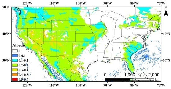
Using the direct-estimation method, the hourly surface broadband albedo based on EPIC was preliminarily obtained. The distribution of the daily averaged estimated shortwave black-sky albedo from EPIC on 4th June 2016 in the study area is shown in Figure 3. The estimated EPIC albedo is mostly concentrated in 0.2–0.3, where the value of 0 represents the area without value because of inversion failure caused by clouds, etc.
4.2. Time Series Analysis of Albedo over Different Land Cover Types
In order to better evaluate the consistency in the time series characteristics of the EPIC albedo, a time series of the EPIC albedo and the ground-based observations, as well as the MODIS albedo, under five different land cover types is shown in Figure 4. The black dots indicate the clear-sky ground-based albedo at local solar noon over the AmeriFlux sites. The red squares indicate the blue-sky albedo extracted from the EPIC daily product. The blue triangular markers indicate the blue-sky albedo from the MCD43A3 product. Generally, the EPIC albedo reflects the trend of the ground-based observations and is comparable to the MODIS albedo. From the comparison results of these sites, it is obvious that the estimated albedo from EPIC is slightly higher than the ground-based observations and the MODIS albedo. This means that the current EPIC albedo has been over-estimated. The over-estimation of the EPIC albedo is more obvious at sites where the land cover type is trees, such as in Figure 4c,d (evergreen needleleaf forests) and Figure 4i,j (woody savannas). Moreover, the EPIC albedo and ground-based observations have better agreement at the sites where the land cover type is that of croplands (Figure 4a,b) or grasslands (Figure 4e,f). The differences between the EPIC albedo and the ground-based observations based on these two land cover types are smaller. It can be seen from these time series changes that at some sites, due to the presence of snow in the spring and winter seasons, the value of the EPIC albedo in the spring and winter is higher than that in the summer and autumn (such as Figure 4a,e). The difference between the EPIC albedo and the ground-based observations is greatest in winter.
4.3. Hourly EPIC Surface Albedo Validation
EPIC provides a high temporal resolution of surface reflectance data, affording the possibility of obtaining hourly surface albedo. In this study, the estimated EPIC albedo in 2016 was compared with the AmeriFlux site observations. Figure 5 shows the comparison of the hourly EPIC albedo and the ground-based observations under different land cover types, and the statistics are given in Table 2. R represents the correlation coefficient, Fit is the equation of the fitted curve, and the color bars and numbers on the right indicate the density of the matching data.
The validation results show that the sites with the land cover types of croplands and grasslands have better consistency with the ground-based observations. The validation results of the sites covered by grasslands show the highest R of 0.82 (Figure 5f), while croplands show the lowest RMSE of 0.03 (Figure 5b). Moreover, the validation results of croplands have the best fit, with Y = 1.04X. Therefore, the difference between the EPIC albedo and the ground-based observations is smaller in terms of grasslands and croplands than the other land cover types.
4.4. Analysis of the Diurnal Variation of the EPIC Surface Albedo
The hourly EPIC albedo and the ground-based observations were investigated to better understand the diurnal variation characteristics of albedo. The number of matches between the EPIC albedo and the ground-based observation data in 2016 was analyzed, and the data with the largest number of matches were concentrated in June. The hourly EPIC albedo in mid-June 2016 was selected in this study, and the diurnal variation of the albedo during that period was analyzed. Meanwhile, the hourly EPIC albedo was compared with the ground-based observations. Figure 6 shows that the effective value of the EPIC albedo is between 6:00 a.m. and 18:00 p.m. in one day. The diurnal variation of the surface albedo shows the same change characteristics under different land cover types. On sunny days, the daily variation curve of the surface shortwave albedo shows a “U” shape, which has the lowest value of albedo at noon and a higher value of albedo in both the morning and evening.
5. Discussion
The comparison and the validation results show that the estimated albedo from EPIC is slightly higher than that of the ground-based observations and the MODIS albedo, mainly because EPIC observes a target from the hotspot direction which has a backscatter peak in the direction when the view and solar directions coincide [34,41]. The over-estimation of the EPIC albedo is more obvious at sites where the land cover type is trees, such as in Figure 4c,d (evergreen needleleaf forests) and Figure 4i,j (woody savannas). This is because vegetation, especially forests, is most affected by the hotspot effect [41]. The differences between the EPIC albedo and the ground-based observations at sites covered by croplands and grasslands are smaller, which is because croplands and grasslands are relatively uniform and are less affected by the hotspot effect of EPIC. Similarly, sites over land cover types of permanent wetlands are less affected by the hotspot effect of EPIC, and the validation results are better than that of sites with the land cover types of evergreen needleleaf forests and woody savannas. Furthermore, the difference between the EPIC albedo, the MODIS albedo, and the ground-based observations is greatest in winter. The main reason is that the albedo of snow cover in the winter changes quickly according to the water content and the freeze-thaw degree of the snow, and the MODIS albedo is lower than the ground-based observations over grasslands and agriculture during snow-covered periods [38].
As the spatial resolution of the EPIC albedo (10 km) is much lower than that of the MODIS albedo product (500 m) or the ground-based observations, some discrepancies may also come from scale mismatch. Even though the selected AmeriFlux site is relatively uniform, while the EPIC albedo has a spatial resolution of 10 km, the spatial differences cannot be ignored. Figure 7 shows the MODIS products (MCD12Q1 and MCD43A3) within 10 km (20 × 20 pixels) of the sites US_Me2 and US_Wkg. Others are shown in Figure S1. We can see that there are some differences in the albedo within 10 km (see as Figure 7b), even over homogeneous sites according to land cover types. When the satellite is directly compared to the ground-based observations, the difference in the space scale brings great differences over those sites with large spatial heterogeneity. Table 3 shows the comparison of the MODIS albedo at the center point, mean value and RMSE within 10 km with the EPIC albedo and the ground-based albedo over ten AmeriFlux sites.
There are also some factors that affect the accuracy of the EPIC albedo based on the direct-estimation method. The calculation of the regression equation coefficients under different land surface cover types depends on the training dataset; therefore, the accuracy of the algorithm is limited by the training dataset [7]. The POLDER3-BRDF product was selected as the training dataset, but the spatial and temporal resolutions of the POLDER3-BRDF and EPIC data are inconsistent, which also affects the estimation accuracy of the EPIC albedo. Therefore, it is necessary to consider the scale effect between different data to improve the estimation accuracy of albedo in future research.
The diurnal variation of surface albedo is related to the solar zenith angle, and the surface albedo decreases as the solar zenith angle decreases. Solar radiation as the denominator when calculating albedo is the strongest in the middle of the day, and so albedo has a minimum value at noon. In addition, the diurnal variation of surface albedo is caused by changes in the atmosphere and the surface through the day, and variations in cloudiness are primarily due to diurnal or synoptic processes [42]. This characteristic of the diurnal variation of surface albedo shows in both ground-based observation and satellite estimations. The same characteristic was found in Bao and Liu’s study [27,28]. The solar zenith angle has a great influence on the albedo over forests when the vegetation grows well or on snowy days [43]. However, the ground-based observations do not change much, while the EPIC albedo shows a “U” shape over trees, as shown in Figure 4c,d (evergreen needleleaf forests) and Figure 4i,j (woody savannas). Hence, the diurnal variation of albedo can be analyzed with the EPIC albedo.
The disadvantage of the direct-estimation method is that it is much more easily affected by sensor noises and cloud detection errors [6,7]. In addition, the prior BRDF database is very important for the direct-estimation algorithm, and the accuracy of the prior BRDF database would impact the albedo estimation significantly. As the surface BRDF obtained from previous retrievals and other products might vary a lot during rapid change periods such as disturbance, etc., it is necessary to check the quality of the BRDF data before using them. The pre-processing steps, such as sensor calibration and cloud mask, and the post-processing steps, such as topographic correction and angular normalization, are also important for deriving surface broadband albedo products.
6. Conclusions
This is the first time that the diurnal albedo from a satellite remote sensing platform (i.e., DSCOVR EPIC) has been obtained, which was shown to greatly improve the temporal resolution of surface albedo. The diurnal variation of the surface albedo from the hourly EPIC albedo exhibits a “U” shape curve, which has the same trend as the ground-based observations. The comparison results show that the EPIC albedo and the ground-based observation data are basically consistent under different land cover types throughout the time series. According to the validation results, the EPIC albedo can achieve better results over grasslands and croplands, with the highest R of 0.82 and the lowest RMSE of 0.03. In sites with land cover types of woody savannas and evergreen needleleaf forests, the albedo is obviously over-estimated, with the slope of the fitted curves above 1.5. In addition, the estimated EPIC albedo over snow-covered surfaces needs to be improved.
The semi-empirical kernel-driven BRDF model is widely used in the retrieval of surface albedo; however, like most other models, the kernel-driven model has poor ability to depict the detailed BRDF shape in the hotspot direction, and thus causes the overestimation of albedo when the observation is in the hotspot direction. The essential reason is the lack of observation data in the direction of the hotspot in the past. EPIC has a unique observational advantage that enables repeated observations in the hotspot direction. Therefore, the accuracy of the BRDF model in the hotspot direction needs to be improved by exploring the advantage of EPIC data when studying the Earth’s surface properties in the future.
EPIC can observe surfaces with high temporal resolution, but the spatial resolution is low. Therefore, it is necessary to combine traditional Earth orbit satellites, first Lagrange Point orbit, and even moon-based observations, to better estimate global surface albedo.
Supplementary Materials
The DSCOVR EPIC surface reflectance products were accessed through the website: https://eosweb.larc.nasa.gov/project/dscovr/dscovr_table. The MODIS products MCD43A3 and MCD12Q1 (V006) were accessed through the website: https://ladsweb.modaps.eosdis.nasa.gov/search/. The AmeriFlux data were downloaded from the website: https://ameriflux.lbl.gov/.
Author Contributions
Q.T. processed and analyzed data and wrote this paper. Q.L. provided important help in the programming for this paper. H.Z. provided useful advice for this paper. L.Y., C.F., Y.C. and Z.L. provided technical assistance for this study. J.G. provided guidance and revised this paper. All authors have read and agreed to the published version of the manuscript.
Funding
This research was funded by the National Natural Science Foundation of China under grant nos. 41590855, 41925019, 41474021 and 41975036, and by the Ministry of Science and Technology of China under grant nos. 2016YFC0200500 and 2016YFA0600302.
Acknowledgments
The authors thank the NASA Earth data Centre (EOSDIS) for maintaining the DSCOVR EPIC surface reflectance products and the MODIS products. The POLDER BRDF datasets were provided by the POSTEL Service Center. The authors acknowledge the following AmeriFlux sites for their data records: US_ARM, US_TW3, US_Me2, US_NC2, US_A32, US_Wkg, US_Srr, US_TW4, US_SRM, and US_Ton. In addition, funding for the AmeriFlux data resources was provided by the U.S. Department of Energy’s Office of Science. The authors would also like to thank the anonymous reviewers for their valuable comments, which greatly improved the quality of this manuscript.
Conflicts of Interest
The authors declare no conflicts of interest.
References
- Dickinson, R.E. Land Surface Processes and Climate—Surface Albedos and Energy Balance. Adv. Geophys. 1983, 25, 305–353. [Google Scholar]
- Manalo-Smith, N.; Smith, G.; Tiwari, S.; Staylor, W. Analytic forms of bidirectional reflectance functions for application to Earth radiation budget studies. J. Geophys. Res. Atmos. 1998, 103, 19733–19751. [Google Scholar] [CrossRef]
- Dickinson, R.E. Land Processes in Climate Models. Remote Sens. Environ. 1995, 51, 27–38. [Google Scholar] [CrossRef]
- Qu, Y.; Liang, S.; Liu, Q.; He, T.; Liu, S.; Li, X. Mapping Surface Broadband Albedo from satellite observations: A review of literatures on algorithms and products. Remote Sens. 2015, 7, 990–1020. [Google Scholar] [CrossRef] [Green Version]
- Wang, K.; Liang, S.; Schaaf, C.L.; Strahler, A.H. Evaluation of Moderate Resolution Imaging Spectroradiometer land surface visible and shortwave albedo products at FLUXNET sites. J. Geophys. Res. Atmos. 2010, 115. [Google Scholar] [CrossRef] [Green Version]
- Liu, Q.; Wang, L.; Qu, Y.; Liu, N.; Liu, S.; Tang, H.; Liang, S. Preliminary evaluation of the long-term GLASS albedo product. Int. J. Digit. Earth. 2013, 6, 69–95. [Google Scholar] [CrossRef]
- Qu, Y.; Liu, Q.; Liang, S.; Wang, L.; Liu, N.; Liu, S. Direct-estimation algorithm for mapping daily land-surface broadband albedo from MODIS data. IEEE Trans. Geosci. Remote Sens. 2013, 52, 907–919. [Google Scholar] [CrossRef]
- Schaaf, C.B.; Gao, F.; Strahler, A.H.; Lucht, W.; Li, X.; Tsang, T.; Strugnell, N.C.; Zhang, X.; Jin, Y.; Muller, J.P. First operational BRDF, albedo nadir reflectance products from MODIS. Remote Sens. Environ. 2002, 83, 135–148. [Google Scholar] [CrossRef] [Green Version]
- Leroy, M.; Deuzé, J.L.; Bréon, F.M.; Hautecoeur, O.; Herman, M.; Buriez, J.C.; Tanré, D.; Bouffiès, S.; Chazette, P.; Roujean, J.L. Retrieval of atmospheric properties and surface bidirectional reflectances over land from POLDER/ADEOS. J. Geophys. Res. 1997, 102, 17023–17037. [Google Scholar] [CrossRef]
- Muller, J.P.; Preusker, R.; Fischer, J.; Zuhlke, M.; Brockmann, C.; Regner, P. ALBEDOMAP: MERIS land surface albedo retrieval using data fusion with MODIS BRDF and its validation using contemporaneous EO and in situ data products. In Proceedings of the 2007 IEEE International Geoscience and Remote Sensing Symposium (IGARSS 2007), Barcelona, Spain, 23–28 June 2007; pp. 2404–2407. [Google Scholar]
- Martonchik, J.V.; Diner, D.J.; Pinty, B.; Verstraete, M.M.; Myneni, R.B.; Knyazikhin, Y.; Gordon, H.R. Determination of land and ocean reflective, radiative, and biophysical properties using multiangle imaging. IEEE Trans. Geosci. Remote Sens. 1998, 36, 1266–1281. [Google Scholar] [CrossRef]
- Rutan, D.; Charlock, T.; Rose, F.; Kato, S.; Zentz, S.; Coleman, L. Global surface albedo from CERES/TERRA surface and atmospheric radiation budget (SARB) data product. In Proceedings of the 12th Conference on Atmospheric Radiation, Madison, WI, USA, 10–14 July 2006. [Google Scholar]
- Grey, W.M.F.; North, P.R.J.; Los, S.O.; Mitchell, R.M. Aerosol optical depth and land surface reflectance from multiangle AATSR measurements: Global validation and intersensor comparisons. IEEE Trans. Geosci. Remote Sens. 2006, 44, 2184–2197. [Google Scholar] [CrossRef]
- Kokhanovsky, A.; Schreier, M. The determination of snow specific surface area, albedo and effective grain size using AATSR space-borne measurements. Int. J. Remote Sens. 2009, 30, 919–933. [Google Scholar] [CrossRef]
- Govaerts, Y.M.; Pinty, B.; Taberner, M.; Lattanzio, A. Spectral conversion of surface albedo derived from Meteosat first generation observations. IEEE Geosci. Remote Sens. Lett. 2006, 3, 23–27. [Google Scholar] [CrossRef]
- Piny, B.; Roveda, F.; Verstraete, M.M.; Gobron, N.; Govaert, Y.; Martonchik, J.V.; Diner, D.J.; Kahn, R.A. Surface albedo retrieval from Meteosat. 1. Theory. J. Geophys. Res. Atmos. 2000, 105, 18099–18112. [Google Scholar] [CrossRef]
- Van Leeuwen, W.J.; Roujean, J.L. Land surface albedo from the synergistic use of Polar (EPS) and Geo-stationary (MSG) observing systems an assessment of physical uncertainties. Remote Sens. Environ. 2002, 81, 273–289. [Google Scholar] [CrossRef]
- Muller, J.P.; López, G.; Watson, G.; Shane, N.; Kennedy, T.; Lewis, P.; Fischer, J.; Guanter, L.; Domench, C.; Preusker, R. The ESA GlobAlbedo project for mapping the Earth’s land surface albedo for 15 years from European sensors. In Proceedings of the 2012 IEEE International Geoscience and Remote Sensing Symposium (IGARSS 2012), Munich, Germany, 22–27 July 2012. [Google Scholar]
- Liang, S.; Zhao, X.; Liu, S.; Yuan, W.; Cheng, X.; Xiao, Z.; Zhang, X.; Liu, Q.; Cheng, J.; Tang, H. A long-term global land surface satellite (GLASS) data-set for environmental studies. Int. J. Digit. Earth 2013, 6, 5–33. [Google Scholar] [CrossRef]
- Lewis, P.; Guanter, L.; Saldana, G.L.; Muller, J.P.; Watson, N.; Shane, N.; Kennedy, T.; Fisher, J.; Domenech, C.; Preusker, R.; et al. The ESA GlobAlbedo project: Algorithm. In Proceedings of the 2012 IEEE International Geoscience and Remote Sensing Symposium (IGARSS 2012), Munich, Germany, 22–27 July 2012. [Google Scholar]
- Di Girolamo, L. Generalizing the definition of the bi-directional reflectance distribution function. Remote Sens. Environ. 2003, 88, 479–482. [Google Scholar] [CrossRef]
- Schaepman-Strub, G.; Schaepman, M.E.; Painter, T.H.; Dangel, S.; Martonchik, J.V. Reflectance quantities in optical remote sensing-definitions and case studies. Remote Sens. Environ. 2006, 103, 27–42. [Google Scholar] [CrossRef]
- Lucht, W.; Roujean, J.L. Considerations in the parametric modeling of BRDF and albedo from multiangular satellite sensor observations. Remote Sens. Rev. 2000, 18, 343–379. [Google Scholar] [CrossRef]
- Govaerts, Y.M.; Wagner, S.; Lattanzio, A.; Watts, P. Joint retrieval of surface reflectance and aerosol optical depth from MSG/SEVIRI observations with an optimal estimation approach: 1 Theory. J. Geophys. Res. 2010, 115. [Google Scholar] [CrossRef]
- Wagner, S.C.; Govaerts, Y.M.; Lattanzio, A. Joint retrieval of surface reflectance and aerosol optical depth from MSG/SEVIRI observations with an optimal estimation approach: 2. Implementation and evaluation. J. Geophys. Res. 2010, 115. [Google Scholar] [CrossRef]
- Liang, S.; Stroeve, J.; Box, J.E. Mapping daily snow/ice shortwave broadband albedo from Moderate Resolution Imaging Spectroradiometer (MODIS): The improved direct retrieval algorithm and validation with Greenland in situ measurement. J. Geophys. Res. 2005, 110. [Google Scholar] [CrossRef] [Green Version]
- Bao, Y.; Lv, S.; Zhang, Y.; Meng, X.; Yang, S. Improvement of surface albedo simulations over arid regions. Adv. Atmos. Sci. 2008, 25, 481–488. [Google Scholar] [CrossRef]
- Liu, X.; Wang, B.; Fu, C. Relationships between surface albedo, soil thermal parameters and soil moisture in the semi-arid area of Tongyu, northeastern China. Adv. Atmos. Sci. 2008, 25, 757–764. [Google Scholar] [CrossRef]
- Grant, I.F.; Prata, A.J.; Cechet, R.P. The impact of the diurnal variation of albedo on the remote sensing of the daily mean albedo of grassland. J. Appl. Meteorol. 2000, 39, 231–244. [Google Scholar] [CrossRef]
- Valero, F.P.J.; Charlson, R.J. Albedo-watching satellite needed to monitor change. Nature 2008, 451, 887. [Google Scholar] [CrossRef]
- Kane, S.R.; Domagal-Goldman, S.D.; Herman, J.R.; Robinson, T.D.; Stine, A.R. Retrieval of planetary rotation and albedo from DSCOVR data. arXiv 2015, arXiv:1511.03779. Available online: https://arxiv.org/abs/1511.03779 (accessed on 8 February 2020).
- Wang, Z.; Schaaf, C.B.; Sun, Q.; Shuai, Y.; Román, M.O. Capturing rapid land surface dynamics with Collection V006 MODIS BRDF/NBAR/Albedo (MCD43) products. Remote Sens. Environ. 2018, 207, 50–64. [Google Scholar] [CrossRef]
- Geiger, B.; Carrer, D.; Franchisteguy, L.; Roujean, J.L.; Meurey, C. Land surface albedo derived on a daily basis from Meteosat second generation observations. IEEE Trans. Geosci. Remote Sens. 2008, 46, 3841–3856. [Google Scholar] [CrossRef]
- Marshak, A.; Herman, J.; Adam, S.; Karin, B.; Carn, S.; Cede, A.; Geogdzhayev, I.; Huang, D.; Huang, L.K.; Knyazikhin, Y.; et al. Earth observations from DSCOVR EPIC instrument. Bull. Am. Meteorol. Soc. 2018, 99, 1829–1850. [Google Scholar] [CrossRef]
- Yang, B.; Knyazikhin, Y.; Mõttus, M.; Rautiainen, M.; Stenberg, P.; Yan, L.; Chen, C.; Yan, K.; Choi, S.; Park, T.; et al. Estimation of leaf area index and its sunlit portion from DSCOVR EPIC data: Theoretical basis. Remote Sens. Environ. 2017, 198, 69–84. [Google Scholar] [CrossRef] [Green Version]
- Lyapustin, A.; Wang, Y.; Laszlo, I.; Hilker, T.; Hall, F.G.; Sellers, P.J.; Tucker, C.J.; Korkin, S.V. Multi-Angle Implementation of Atmospheric Correction for MODIS (MAIAC). 3: Atmospheric Correction. Remote Sens. Environ. 2012, 127, 385–393. [Google Scholar] [CrossRef]
- Vasilkov, A.; Lyapustin, A.; Mitchell, B.G.; Huang, D. UV Reflectance of the ocean from DSCOVR/EPIC: Comparisons with a theoretical model and Aura/OMI observations. J. Atmos. Ocean. Technol. 2019, 36, 2087–2099. [Google Scholar] [CrossRef]
- Wang, Z.; Schaaf, C.B.; Strahler, A.H.; Chopping, M.J.; Román, M.O.; Shuai, Y.; Woodcock, C.E.; Hollinger, D.Y.; Fitzjarrald, D.R. Evaluation of MODIS albedo product (MCD43A) over grassland, agriculture and forest surface types during dormant and snow-covered periods. Remote Sens. Environ. 2014, 140, 60–77. [Google Scholar] [CrossRef] [Green Version]
- Sulla-Menashe, D.; Gray, J.M.; Abercrombie, S.P.; Friedl, M.A. Hierarchical mapping of annual global land cover 2001 to present: The MODIS Collection 6 Land Cover product. Remote Sens. Environ. 2019, 222, 183–194. [Google Scholar] [CrossRef]
- Liu, Y.; Wang, Z.; Sun, Q.; Erb, A.M.; Li, Z.; Schaaf, C.B.; Zhang, X.; Román, M.O.; Scott, R.L.; Zhang, Q. Evaluation of the VIIRS BRDF, albedo and NBAR products suite and an assessment of continuity with the long term MODIS record. Remote Sens. Environ. 2017, 201, 256–274. [Google Scholar] [CrossRef]
- Hapke, B.; DiMucci, D.; Nelson, R.; Smythe, W. The cause of the hot spot in vegetation canopies and soils: Shadow-hiding versus coherent backscatter. Remote Sens. Environ. 1996, 58, 63–68. [Google Scholar] [CrossRef] [Green Version]
- Rutan, D.A.; Smith, G.L.; Wong, T. Diurnal variations of albedo retrieved from earth radiation budget experiment measurements. J. Appl. Meteorol. Climatol. 2014, 53, 2747–2760. [Google Scholar] [CrossRef]
- Liu, J.; Schaaf, C.; Strahler, A.; Jiao, Z.; Shuai, Y.; Zhang, Q.; Roman, M.; Augustine, J.A.; Dutton, E. Validation of moderate resolution imaging spectroradiometer (MODIS) albedo retrieval algorithm: Dependence of albedo on solar zenith angle. J. Geophys. Res. Atmos. 2009, 114. [Google Scholar] [CrossRef]
Figure 1.
Land cover map of the study area from MCD12Q1 based on the International Geosphere-Biosphere Program (IGBP) classification and the AmeriFlux sites used in this study. 1 indicates that the land cover type is ENF (evergreen needleleaf forests), 2: EBF (evergreen broadleaf forests), 3: DNF (deciduous needleleaf forests), 4: DBF (deciduous broadleaf forests), 5: MF (mixed forests), 6: CSH (closed shrublands), 7: OSH (open shrublands), 8: WSA (woody savannas), 9: SAV (savannas), 10: GRA (grasslands), 11: WET (permanent wetlands), 12: CRO (croplands), 13: UBL (urban and built-up Lands), 14: CRO/NVM (cropland/natural vegetation mosaics), 15: PSI (permanent snow and ice), 16: barren, 17: water bodies, 0: unclassified.

Figure 2.
Flowchart for estimating surface broadband albedo from the Earth Polychromatic Imaging Camera (EPIC).
Figure 2.
Flowchart for estimating surface broadband albedo from the Earth Polychromatic Imaging Camera (EPIC).

Figure 3.
Daily averaged shortwave black-sky albedo from EPIC on 4 June, 2016 in the study area. 0 represents the area without value because of inversion failure caused by clouds, etc.
Figure 3.
Daily averaged shortwave black-sky albedo from EPIC on 4 June, 2016 in the study area. 0 represents the area without value because of inversion failure caused by clouds, etc.

Figure 4.
Time series of albedo under different typical land cover types in 2016 from EPIC, MODIS, and AmeriFlux. The land cover type of (a,b) is croplands, (c,d) is evergreen needleleaf forests, (e,f) is grasslands, (g,h) is permanent wetlands, and (i,j) is woody savannas. DOY means day of the year.


Figure 5.
Validation results of hourly EPIC albedo over different land cover types in 2016. The land cover type of (a,b) is croplands, (c,d) is evergreen needleleaf forests, (e,f) is grasslands, (g,h) is permanent wetlands, and (i,j) is woody savannas. The color bars and numbers on the right indicate the density of the matching data. RMSE, root mean square error; RMB, relative mean bias; MAE, mean absolute error; MBE, mean bias error.


Figure 6.
Analysis of the diurnal variation of EPIC albedo over different land cover types. The land cover type of (a,b) is croplands, (c,d) is evergreen needleleaf forests, (e,f) is grasslands, (g,h) is permanent wetlands, and (i,j) is woody savannas. The date of (a,e) is 16th June 2016; (b,g), (h) is 12th June 2016; (c) is 15th July 2016; (d) is 8th June 2016; (f) is 18th June 2016; (i) is 19th June 2016; and (j) is 20th June 2016.


Figure 7.
Land cover map from MCD12Q1 (a) and MCD43A3 blue-sky albedo (b) over US_Me2, land cover map (c) and MCD43A3 blue-sky albedo (d) over US_Wkg on 4th June, 2016. 1 indicates that the land cover type is ENF (evergreen needleleaf forests), 5: MF (mixed forests), 7: OSH (open shrublands), 9: SAV (savannas), 10: GRA (grasslands). The AmeriFlux sits are located at the center of each map.


Table 1.
The information of the AmeriFlux sites used in this study.
| Land Cover Type | Site Name | Longitude (°) | Latitude (°) |
|---|---|---|---|
| Croplands | US_ARM | −97.4888 | 36.6058 |
| US_TW3 | −121.6467 | 38.1159 | |
| Evergreen Needleleaf Forests | US_Me2 | −121.5574 | 44.4523 |
| US_NC2 | −76.6685 | 35.8030 | |
| Grasslands | US_A32 | −97.8198 | 36.8193 |
| US_Wkg | −109.9419 | 31.7365 | |
| Permanent Wetlands | US_Srr | −122.0264 | 38.2006 |
| US_TW4 | −121.6414 | 38.1030 | |
| Woody Savannas | US_SRM | −110.8661 | 31.8214 |
| US_Ton | −120.9659 | 38.4316 |
Table 2.
Statistics comparing the AmeriFlux ground-based measurements with the EPIC albedo.
| Land Cover Type | Site Name | Number of Matching Points | R | R2 | RMSE | Fit |
|---|---|---|---|---|---|---|
| CRO | US_ARM | 441 | 0.68 | 0.4624 | 0.08 | Y = 1.41X − 0.01 |
| CRO | US_TW3 | 343 | 0.69 | 0.4761 | 0.03 | Y = 1.04X |
| ENF | US_Me2 | 335 | 0.76 | 0.5776 | 0.09 | Y = 1.85X + 0.01 |
| ENF | US_NC2 | 311 | 0.55 | 0.3025 | 0.10 | Y = 1.64X + 0.03 |
| GRA | US_A32 | 311 | 0.79 | 0.6241 | 0.05 | Y = 1.32X − 0.03 |
| GRA | US_Wkg | 740 | 0.82 | 0.6724 | 0.10 | Y = 1.58X |
| WET | US_Srr | 607 | 0.68 | 0.4624 | 0.07 | Y = 0.94X + 0.08 |
| WET | US_TW4 | 425 | 0.74 | 0.5476 | 0.11 | Y = 1.20X + 0.08 |
| WSA | US_SRM | 477 | 0.47 | 0.2209 | 0.14 | Y = 1.67X + 0.03 |
| WSA | US_Ton | 640 | 0.68 | 0.4624 | 0.11 | Y = 1.93X − 0.04 |
Table 3.
Comparison of the MODIS albedo, the EPIC albedo and the ground-based albedo over the AmeriFlux sites on 4th June 2016.
Table 3.
Comparison of the MODIS albedo, the EPIC albedo and the ground-based albedo over the AmeriFlux sites on 4th June 2016.
| Site Name | MODIS Albedo (Center Point) | MODIS Albedo (Mean Value Within 10 km) | MODIS Albedo (RMSE Within 10 km) | EPIC Albedo | Site Albedo |
|---|---|---|---|---|---|
| US_ARM | 0.166 | 0.155 | 0.009 | 0.201 | 0.170 |
| US_TW3 | 0.212 | 0.169 | 0.033 | 0.165 | 0.157 |
| US_Me2 | 0.075 | 0.079 | 0.004 | 0.226 | 0.098 |
| US_NC2 | 0.130 | 0.142 | 0.012 | 0.220 | 0.091 |
| US_A32 | 0.138 | 0.146 | 0.009 | 0.215 | 0.171 |
| US_Wkg | 0.133 | 0.157 | 0.023 | 0.253 | 0.159 |
| US_Srr | 0.212 | 0.169 | 0.033 | 0.165 | 0.157 |
| US_TW4 | 0.212 | 0.169 | 0.033 | 0.165 | 0.157 |
| US_SRM | 0.194 | 0.204 | 0.020 | 0.284 | 0.157 |
| US_Ton | 0.207 | 0.187 | 0.021 | 0.280 | 0.131 |
© 2020 by the authors. Licensee MDPI, Basel, Switzerland. This article is an open access article distributed under the terms and conditions of the Creative Commons Attribution (CC BY) license (http://creativecommons.org/licenses/by/4.0/).
Share and Cite
MDPI and ACS Style
Tian, Q.; Liu, Q.; Guang, J.; Yang, L.; Zhang, H.; Fan, C.; Che, Y.; Li, Z. The Estimation of Surface Albedo from DSCOVR EPIC. Remote Sens. 2020, 12, 1897. https://doi.org/10.3390/rs12111897
AMA Style
Tian Q, Liu Q, Guang J, Yang L, Zhang H, Fan C, Che Y, Li Z. The Estimation of Surface Albedo from DSCOVR EPIC. Remote Sensing. 2020; 12(11):1897. https://doi.org/10.3390/rs12111897
Chicago/Turabian StyleTian, Qiuyue, Qiang Liu, Jie Guang, Leiku Yang, Hanwei Zhang, Cheng Fan, Yahui Che, and Zhengqiang Li. 2020. "The Estimation of Surface Albedo from DSCOVR EPIC" Remote Sensing 12, no. 11: 1897. https://doi.org/10.3390/rs12111897
Note that from the first issue of 2016, this journal uses article numbers instead of page numbers. See further details here.