Distribution Consistency Loss for Large-Scale Remote Sensing Image Retrieval

1
College of Computer Science and Technology, Jilin University, Changchun 130012, China
2
Key Laboratory of Symbolic Computation and Knowledge Engineering of Ministry of Education, Jilin University, Changchun 130012, China
3
Editorial Department of Journal (Engineering and Technology Edition), Jilin University, Changchun 130012, China
*
Author to whom correspondence should be addressed.
Remote Sens. 2020, 12(1), 175; https://doi.org/10.3390/rs12010175
Submission received: 24 November 2019
/
Revised: 28 December 2019
/
Accepted: 30 December 2019
/
Published: 3 January 2020
(This article belongs to the Special Issue Content-Based Remote Sensing Image Retrieval)
Abstract
:Remote sensing images are featured by massiveness, diversity and complexity. These features put forward higher requirements for the speed and accuracy of remote sensing image retrieval. The extraction method plays a key role in retrieving remote sensing images. Deep metric learning (DML) captures the semantic similarity information between data points by learning embedding in vector space. However, due to the uneven distribution of sample data in remote sensing image datasets, the pair-based loss currently used in DML is not suitable. To improve this, we propose a novel distribution consistency loss to solve this problem. First, we define a new way to mine samples by selecting five in-class hard samples and five inter-class hard samples to form an informative set. This method can make the network extract more useful information in a short time. Secondly, in order to avoid inaccurate feature extraction due to sample imbalance, we assign dynamic weight to the positive samples according to the ratio of the number of hard samples and easy samples in the class, and name the loss caused by the positive sample as the sample balance loss. We combine the sample balance of the positive samples with the ranking consistency of the negative samples to form our distribution consistency loss. Finally, we built an end-to-end fine-tuning network suitable for remote sensing image retrieval. We display comprehensive experimental results drawing on three remote sensing image datasets that are publicly available and show that our method achieves the state-of-the-art performance.
1. Introduction
With the rapid advancement of aerospace and remote sensing technology, the comprehensive observation capability of the earth has been greatly improved. The available remote sensing images have undergone tremendous changes in terms of improved spatial resolution and improved acquisition rates, which has imposed a profound impact on the way we process and manage remotely sensed images. The increased spatial resolution provides a new opportunity to advance the analysis and understanding of remotely transmitted images. The ever-increasing data collection speed allows us to collect large amounts of remote sensing data every day, but this poses a huge challenge for managing large datasets, especially how to quickly access the data of interest.
The early remote sensing image retrieval system only provides a text-based retrieval interface, and the image is described by related text information, such as image name, geographic region and acquisition time. However, the information does not have direct relation to the visual content of the image. To solve this problem, people are working on content-based image retrieval (CBIR). CBIR is a branch of image retrieval and is a useful technique for quickly retrieving data of interest from a massive database, by extracting features (such as colors and textures) in the visual content and identifying similar or matching images in the database. In recent years, based on the advantages of CBIR, the remote sensing community has invested a lot of energy to make CBIR suitable for remote sensing image retrieval. Henceforth, image retrieval based on remote sensing images has attracted numerous scholarly studies and has achieved huge progress [1,2].
In particular, remote sensing is centered on developing effective methods to extract features because the retrieval performance largely depends on feature effectiveness. The key issue in CBIR is to find the underlying distinctiveness from the image. Traditional feature extraction techniques rely primarily on manual design features. Their design is subject to human intervention, subjective and makes it difficult to express high-level semantic information. Handcrafted features are also commonly used as remote sensing image representations in RSIR work [3,4], including spectral features [5], shape features [6] and texture features [7]. Compared with low-level features, middle-level features embed low-level feature descriptor into the encoded feature space, and use more compact feature vectors to represent complex image textures and structures. The typical methods are BoW (Bag of Word) [4], VLAD (Vector of Aggregate Locally Descriptor) [1] and FV (Fisher Vector) [2].
However, the abovementioned underlying features and middle-level features still have a “semantic gap” with high-level features. The above feature extraction method is based on the characteristics of artificial design and has limitations on the expression ability of remote sensing image content. The advancement of deep learning has driven content-based image retrieval. It abstracts feature vectors trained by a large amount of data and automatically learns the rich information contained in the data. It has been proven that deep learning has better performance than traditional manual features in image retrieval of remote sensing images [2,8,9]. Moreover, deep learning solves a variety of computer vision barriers as well as remote sensing issues, such as simultaneous extraction of roads and buildings, ultra-high-resolution optical images and hyperspectral image classification. The essence of deep learning is to discover the complex structure of the dataset by training a large amount of data. The rich information contained in the automatic learning data is abstracted into a feature vector, so that handcrafted features are not needed in remote sensing images. In the context of remote sensing image big data, deep learning technology is of great value in image retrieval of massive remote sensing data.
Deep metric learning represents a newly emerging technology that combines metric learning with deep learning. A deep neural network deploys its discriminative power to embed the image into metric space. Simple metrics, including cosine similarity and Euclidean distance, can be directly used to measure the similarity between images [10]. In recent years, deep learning has achieved great success in application areas, which include target recognition, target detection, image segmentation and natural language understanding [11,12,13], and has been gradually applied in the field of image retrieval, such as landmark image retrieval [14], natural image retrieval [14] and face recognition [10]. Despite apparent differences between remote sensing images and ordinary natural images, DML presents huge potential in content-based image retrieval of remote sensing images [15].
The loss function is crucial in the success of DML, and various loss functions have been proposed in the literature. Contrastive loss [16] records the relationship between pairs of data points by zooming in on similar samples and pushing far from dissimilar samples. The triplet loss [17] consists of an anchor point, a similar (positive) data point and dissimilar (negative) data points. It learns a distance metric that allows anchor points to be closer to similar points than dissimilar points. Because of the relationship between the positive and negative pairs, triplet loss is usually better than contrastive loss [10,18] and, inspired by this, recent works [18,19,20,21,22] proposed to consider the relationship between multiple data points, where good performance is achieved in applications such as retrieval and classification.
However, there are still some limitations in the current state of DML on remote sensing image retrieval. First, we noticed that sample mining only uses part of the positive sample information, and the differences between sample categories are ignored. Secondly, we observe that the previous loss treats each positive sample equally, thus neglecting the sample differences within the category on the loss calculation; that is, the effect of the quantity of relationships between easy samples and hard samples on the loss optimization. This deficiency affects the quality of image retrieval, especially remote sensing image retrieval. When magnifying the pictures in the remote sensing dataset, we found that the sample differences within each category are different. The specific differences are shown in Figure 1. The differences within the categories in Figure 1a,b are small, and the texture features and color characteristics are similar, but the differences within the categories in Figure 1c,d are relatively large. After comparison, we find that the selected hard positive samples deserve a larger weight because it has a larger contribution to the loss when the samples have larger differences within categories, namely the larger proportion of hard samples. Therefore, different categories should be assigned different weights when performing positive sample mining. Ideally, a hard sample with a large percentage should be given a greater weight.
Our major contributions in this study are listed as follows:
- For the remote sensing image retrieval task, we propose a novel distribution consistency loss (DCL), to learn discriminative embeddings. Different from the previous pair-based loss, it performs loss optimization based on the difference in the number of samples within the class and the sample distribution structure between the classes. It includes the sample balance loss obtained by assigning dynamic weights to selected hard samples based on the ratio of easy sample and hard sample in the class, and the ranking consistency loss weighted [23] according to the distribution of the category of the negative sample.
- A sample mining method suitable for a remote sensing method is proposed. The intra-class hard sample mining method is used to select five positive samples, and each positive sample is given a dynamic weight. The hard class is used instead of hard content mining. This method selects a representative sample which obtains richer information while increasing the speed of convergence.
- We built an end-to-end fine-tuning network architecture for remote sensing image retrieval, which applied convolutional neural network, and selected the most suitable method for remote sensing image retrieval. In DCL, the loss and gradients were computed based on sum-pooling (SPoC) [24] features. The loss function influences the activation distribution of the feature response map, which enhanced accurate saliency and extracted more discriminative features. In addition, we also compared different combinations of image multi-scale processing, whitening and query expansion, and finally selected the most suitable multi-scale cropping method to process the input data.
2. Related Work
In this section, we will first give the formulation of the remote sensing image retrieval method, and then introduce the existing general pair-based weighting loss. Finally, we introduce the sample mining method in metric learning.
2.1. Remote Sensing Image Retrieval Methods
The performance of remote sensing image retrieval mainly depends on the expressive power of image features. In the past ten years, people have made great efforts to extract effective features and construct remote sensing image scene datasets [9]. Compared with the traditional feature extraction method, the development of deep learning has greatly improved the quality of image feature extraction. In the context of remote sensing image big data, it is possible to extract remote sensing image features by learning from massive remote sensing image data. Therefore, the use of deep learning methods to improve the accuracy of remote sensing image retrieval tasks has a very broad prospect.
At present, the remote sensing image retrieval method based on deep learning generally uses convolutional neural networks (CNNs) to extract the features of remote sensing images, and trains the network by means of classification. Finally, remote sensing image retrieval is performed through the features extracted by the network [26]. In order to obtain more discriminative features, the two dimensions of channel and space are weighted to obtain significant features [27]. The pre-trained RSIR method uses a trained overfeat network to extract RS features. The outputs of the seventh layer (DN7) [28] and the eighth layer (DN8) [29] are considered as deep features. Yang uses the S-BOW [4] feature to represent the RS image, and selects the L1 norm distance to determine the similarity of the image. The similarity between RS images is converted into the similarity between blur vectors by region-based fuzzy matching (RFM) [30]. Xu discovered useful information of RS images through similarity. With the help of deep learning technology, he designed a feature learning method named Deep BOW under the bag of words model [31]. In addition to feature weighting, a saliency module can be added to extract convolutional layer aggregation features of multiple scales [31], or to add attention mechanisms and local convolution features [30] to achieve more accurate remote sensing image retrieval. However, the above methods require a large amount of training data. For some remote sensing image targets, the number of training images that can be obtained is small, and the deep learning training data requirements cannot be met. At the same time, the characteristics of the remote sensing image target rotation are not taken into consideration, which makes the current deep learning model inconsistent or even different for different rotation angle target features, resulting in low retrieval accuracy of remote sensing images.
Due to the large number of remote sensing images, the general linear search method is far from meeting the time performance requirements of large-scale remote sensing image retrieval and is replaced by the approximate nearest neighbor (ANN). The basic idea of ANN is to replace the exact match with the approximate optimal, and this greatly improves the retrieval efficiency while ensuring the accuracy of image retrieval. Among them, the hash learning method [32] is a commonly used method of ANN. The hash learning method is widely used in large-scale image retrieval due to its advantages in speed and storage. For example, the non-linear hashing method based on RS two kernels, achieves real-time search and fast detection through mapping image feature vectors of high dimensional image into compact truncated hash codes [32]. A hashing-based approach introduces a hashing algorithm to encode RS images [31]. However, hash learning methods typically require longer hash codes to achieve satisfactory accuracy, which results in larger storage space requirements and retrieval efficiency issues. However, with a shorter hash code, there is a problem that the retrieval recall rate is low.
In recent years, deep learning methods have also been applied to hash coding to obtain better coding effects [33]. The partial random hash of the random projection is generated in an unsupervised manner, the image is mapped to the Hamming space to obtain the low-latitude expression of the image, and then the model is trained [32]. Unsupervised strategies [15], metric-based learning of the Hash network [34], and deep hash neural networks [33] are also methods for resolving large-scale remote sensing images. Through these deep learning-based hashing methods, the image can directly obtain the corresponding hash encoding. However, in order to minimize the loss of feature information of the image, the hash coding dimension is often very high, and it is necessary to traverse the entire data set when performing image retrieval, resulting in low retrieval efficiency.
Based on the excellent performance on ImageNet [35] and other issues, convolutional neural networks (CNNs) combined with metric learning are the most effective deep learning methods in image retrieval. However, training a valid CNN from scratch requires a lot of markup images. Using CNN pre-trained on ImageNet as a feature extractor, we can learn specific features by fine-tuning CNNs that are pre-trained on the target dataset, so translate learning is often used to solve the problem of lacking enough markup images. This is very helpful in some areas where large-scale publicly available datasets are not enough, such as remote sensing. In [36], Penatti studied the generalization ability of deep features extracted by CNN by extracting and transferring deep features from everyday objects to remote sensing. Experimental results indicate that transfer learning is an effective method for cross-domain tasks. There are many pre-trained CNNs for migration learning, such as the Caffe Reference model (CaffeRef) [37], the baseline model AlexNet [38], the VGG network [39], the newly developed deeper model GoogLeNet [40], and the Residuals Network (ResNet) [41].
Recently, these pre-trained CNNs and their modified versions have been widely applied in different image retrieval tasks, ranging from computer vision [42,43,44] to remote sensing [2,45]. Chaudhuri et al. [46] put forward the SGCN architecture for evaluating the similarity between paired graphs that are trained for CBIR by contrastive loss function. Famao et al. [47] use two image-to-class distances to re-rank the initial retrieval result, referred to as the similarity between an image and an image class. For different tasks, people have made some improvements in various stages of the search. Bindita et al. [48] solve multilabel RS image retrieval problems drawing on a semi-supervised graph-theoretic method and expensive and time-consuming problems by multi-label annotation images. Babenko and Lempitsky [24] form image signatures through aggregating deep convolutional descriptors by sum-pooling of convolutional features (SPoC). Tolias et al. [49] used many multi-scale overlapping regions of the last convolutional feature map to extract the maximum activations of convolutions (MAC). In [50], a trainable generalized mean (GeM) pool layer replaces the MAC layer. This greatly improves retrieval accuracy. A new CNN architecture has recently been proposed in [51], which can learn and extract multi-scale local descriptors in the salient regions of images. RSIR can be viewed as a branch of image retrieval. They are still identified by visual content based on similar images. However, due to the particularity of RS images, it may not be suitable for the direct deployment of some commonly used technologies. In this paper, we will compare the commonly used techniques and build the most suitable retrieval method for remote sensing images.
2.2. General Pair-Based Weighting Loss
This section will explicitly review some typical pair-based weighting losses, including contrastive loss [52], triplet loss [17], N-pair loss [19], binomial deviance loss [53], lifted structured loss [18] and multi-similarity loss [54].
2.2.1. Contrastive Loss
Based on the selected paired positive (samples belonging to the same class of the query sample) and negative (samples not belonging to the same class of the query sample) samples, the contrastive loss [16] is designed to minimize the distance between the query sample and the positive sample pair, while maximizing the distance between the query image and the negative sample pair, restricted within a predefined margin α,
where is the whole paired distance set, in which in Equation (1) ( are the -normalized SPoC vector of image a and image b respectively). indicates whether a pair is from the same class , in which is the positive paired distance set, and stands for the negative paired distance set. Besides, is the hinge function, and α is a threshold parameter designed according to actual needs.
2.2.2. Triplet Loss
In view of triplet data triplet loss [17] is designed to learn a deep embedding, which widens the distance between negative pairs and makes the distance larger than that of a randomly selected positive one over a margin α,
Concretely, the equal weight for all the selected pairs is assigned by the given triplet loss.
2.2.3. N-Pair Loss
Triplet loss pulls close a positive sample while pushing away a negative sample. Only three samples are in a batch that participates in the training. N-pair loss [55] increases the number of negative samples that interact with the query sample to improve the performance of triplet loss. It takes advantage of all sample pairs in the mini-batch and learns more differentiated representations based on structural information between the data. In detail, the sample includes one positive sample and negative samples selected from other different categories, which suggests one negative sample per category, and the loss function is listed as follows:
where and the distance of a positive pair and is . However, the sample in N-pair loss is assigned the same weight for both the positive and negative pair in a triplet, and its weight value is
2.2.4. Binomial Deviance Loss
Unlike the hinge function, Dong et al. introduced the binomial deviance loss using the soft plus function in the contrastive loss [53]:
As for anchor, and indicates the number of positive and negative sample pairs, and , and are fixed hyper-parameters.
We derive the positive and negative sample pairs in Equation (5), and the weights are as follows:
2.2.5. Lifted Structured Loss
Different from using merely one negative sample in each class, the loss of lifted structure loss [18] relies on the advantages of training batches of minibatch SGD training, and uses random sampled image pairs or triples, constructing training batches to calculate the loss of each pairs or triplets. The loss function is given as a log-sum-exp formulation:
As for a query sample, lifted structured loss explores structural relationships by identifying a positive sample from all negative samples of a mini-batch. For positive sample pairs, the weight of lifted structured loss is
The weight of the negative sample pair is
2.2.6. Multi-Similarity Loss
Based on binomial deviance loss and lifted structured loss, multi-similarity loss [33] defines self-similarity and relative similarity, and proposes a general weighting strategy that takes advantage of both positive and negative sample pairs. The loss is calculated as follows:
where , and are hyperparameters used to control different pairs of weights. For positive and negative samples, the weights set for multi-similarity loss are
The aforementioned contrastive loss, triplet loss and N-pair loss give the same weight to the positive and negative sample pairs. Unlike them, Equations (6) and (7) show that binomial deviance loss considers self-similarity, and lifted structure loss sets weights for positive and negative sample pairs according to the negative relative similarity as in Equations (9) and (10). Multi-similarity loss combines the distribution of the sample itself and the surrounding samples, taking into account the self-similarity and relative similarity of the sample pairs. However, this approach ignores the distribution of samples within the class and the differences between different classes.
2.3. Sample Mining
Many of the loss functions of metric learning are built on top of sample pairs or sample triples, so the sample space is of very large magnitude. In general, there exist apparent difficulties for the model to exhaustively learn all pairs of samples during the training process, and the amount of information for most sample pairs or sample triples is small. Especially in the later stages of model training, the gradient values on these sample pairs or sample triples are almost zero. Without any targeted optimization, the convergence speed of the learning algorithm will be slow and easy to fall into the local optimum. This is not conducive to better characterization of network learning, and sample mining plays a key role in metric learning.
Hard sample mining is an important means to speed up the convergence of learning algorithms, improves the generalization ability of the network and the learning effect [10,56,57]. TriHard loss [17] is a kind of online sampling method for hard samples based on a training batch, which is improved on the basis of triple loss. For each batch, select one of the hardest positive samples and one of the hardest negative samples as an anchor point to form a triple, although this method produces only a small number of triples. When we need enough triples, we usually need a larger batch [10]. MAML [58] only selects the most hard positive sample pair and the most hard negative sample pair for each picture in the batch, which is a hard sample that is harder than TriHard. In addition, it also considers the relative distance and absolute distance, and the performance is better than TriHard loss. N-pair loss considers the query sample and the negative samples of several other different classes in each parameter update process, which speeds up the convergence of the model. Lifted structure loss is based on all positive and negative sample pairs in a mini batch to calculate loss. The triplet of the triplet loss is determined in advance, and all negative samples are considered during the construction process. Proxy NCA loss [22] selects a sample closest to a small portion of the data in the training set as a proxy when sampling. For ranked list loss [59], the sampling strategy is to select samples whose loss function is not zero. Although all samples within the threshold were mined, the differences between the negative sample classes and the effects of surrounding samples were not considered.
We fully consider the diversity and difference of samples, select multiple positive samples and negative samples of different types, as well as set the distance from the sample according to the distribution of the neighbor samples around the negative samples. Figure 2 shows a comparison of our method with other different methods.
3. Methodology
In this section, we describe how to develop a positive and negative sample mining strategy to make full use of the effective training of sample information, and then design a weighted approach of positive (negative) sample pairs based on positive (negative) sample characteristics. Finally, we propose a novel and effective metric learning loss function.
We set as the input data, where represent the i-th image and is the label of the corresponding class. The total number of classes is C, where . Then an instance is projected onto a unit sphere in a l-dimension space by :, where f is a neural network parameterized by . Let be the images in the c-th class, where the total number of images is . Our purpose is to learn a discriminative function to represent a higher similarity between positive sample pairs and a lower similarity between negative sample pairs.
Therefore, there are at least two images in each category in order to evaluate all categories. In this case, we aim to find a paired sample from other samples in the same category.
3.1. Distribution Consistency Loss
As shown in Figure 3, our distribution consistency loss consists of two parts. The first part is for the sample balance loss of positive samples (the so-called sample balance refers to the ratio of the number of hard positive samples and easy positive samples), and the second part is for the ranking of consistency loss of negative samples. The ranking consistency here is to maintain the true distribution between classes by learning the ranking of the categories of each negative sample. The specific details are as follows.
3.1.1. Sample Mining
Sample mining can achieve rapid convergence of networks and improve network performance. It is widely used in metric learning [10,17,19,60,61,62,63]. Given a query sample , in order to mine the positive and negative samples, we first use the currently effective network [50] to extract the image features, and use the extracted features to calculate the Euclidean distance between all samples and the query sample and do the ranking based on the distance. We define as a collection of the same category with the query image, which is expressed as , . is a collection of other images, represented as , We create a dataset of tuples , where represents the query image, is the positive set selected from , and is the negative set selected from . The training image pairs consist of these tuples, where each tuple corresponds to positive sample pairs and negative sample pairs.
Positive set : For the query sample , we select the in-class samples (hard samples) that are furthest from it as positive samples.
Negative set : For negative samples, in order to learn the differences between classes, negative “class” mining is proposed against negative “instance” mining, which greedily selects a negative class in a relatively efficient manner. In particular, we select the nearest negative sample based on the distance between the query sample and all samples; that is, the sample that has the highest similarity to the query sample but belongs to a different category from the query sample. Next, we look for the second closest sample. When this sample belongs to the same class as the previously found sample, the sample is discarded and the searching will continue, otherwise it will be the second negative sample, and so on, until we choose negative samples from classes.
Hard sample in positive sample weight: In the weighting process of positive samples, we delineate a hard sample boundary in the positive sample to reduce the influence of the number relationship between easy and hard in the positive sample. Assume is the query sample, a hard and positive pair is selected if satisfies the condition
where we define the similarity of the two samples as , where resulting in an similarity matrix; whose element at is ; and is a hyperparameter. The number of hard positive samples satisfying the above constraints is represented by .
3.1.2. Distribution Consistency Loss Weighting
Through the sample mining strategy, we can select samples with representative information and discard samples with less information. We developed different soft weighting schemes for positive and negative sample pairs.
For positive sample pairs, our weighting mechanism relies on the number and distribution of easy and hard samples within the class. For an anchor, the more the number of hard samples in the class, the more information is included in the selected positive sample pair. In the process of training, we give a large weight to the sample pairs. When the number of hard samples in the class is small, the selected hard samples may be noise or the information carried is not representative. If a large weight is given at this time, the overall learning direction of the model may be deviated, resulting in invalid learning. Therefore, for classes with a small number of hard samples, we assign less weight to the selected sample pairs. Specifically, given a selected positive pair its weight can be computed as
where is a hyperparameter.
For negative samples, we use the weight of the distribution entropy [23] to maintain the similarity ranking consistency of the class. The distribution entropy define the weight value as .
3.1.3. Optimization Objective
For each query , we assign the weighted defined by the quantity relationship between the hard sample and the easy sample in the class of the selected positive sample, and we use a margin m to make it closer to its positive set than to its negative set . Moreover, we compel all negative samples to be farther than a dynamic boundary . This threshold is determined by the similarity between the negative samples selected from the different classes and the query picture. Thus, all samples from the same class were pulled into a hypersphere.
We attempt to pull all non-trivial positive points in together and learn a class hypersphere by minimizing:
where and represent the feature vectors of images and , respectively, and represents the Euclidean distance between and . Similarly, we intend to push all non-trivial negative points in beyond the boundary , by minimizing:
In DCL, we treat the two minimization objectives equally and optimize them jointly:
we update according to weighted combination of other elements.
For the learning of deep models, we do DCL based on a stochastic gradient descent and mini-batch. Each minibatch represents a randomly sampled subset in the whole training classes. Every image in the mini-batch serves as the query (anchor) iteratively, and the other images act as the gallery. We represent the DCL of each mini-batch as
The batch size is represented by N. We clarify the DCL-based learning of the deep embedding function f in Figure 4.
4. Experiments and Discussion
In this section, we discuss in detail the application dataset, the retrieval performance metrics for quantitative evaluation and the experimental hardware conditions. Then, the relevant parameters related to the model are mined. Finally, we assessed different combinations of network settings and compared them with the current methods. In this experiment, our proposed method is applicable to all convolutional neural networks. For model training, we used the pytorch deep learning architecture to train the DCL-based deep network model. We initialized the parameters of the network by the weights of the corresponding networks pre-trained on ImageNet [35]. Due to the use of network pre-training parameters [64], the momentum was 0.9 for the VGG16 and Resnet50 networks during training. The experimental environment was an Intel Xeon(R) CPU E5-2620 V3, GPU with 12 GB of memory, NVIDIA(R) Titan X graphics card, driver version 419.**, operating system Ubuntu 18.04 LTS, pytorch version v1.0.0, CUDA version 10.0 and cudnn version 7.5.
4.1. Experimental Settings
4.1.1. Datasets
To test the proposed method, we use two publicly available RSIR datasets, the UC Merced dataset (UCMD) [24], PatternNet [9] and the NWPU-RESISC45 dataset [25]. To avoid over-fitting of the feature extraction network, we conducted the image retrieval task under zero-shot settings, in which the training dataset and testing dataset contain image classes without no intersection.
UCMD [24] is a classification dataset for land use and cover. It contains 21 classes, each with 100 images. Examples from every class are shown as follows: building, agricultural, golf course, baseball diamond, medium density residential, parking lot, beach, freeway, chaparral, intersection, mobile home park, river, overpass, airplane, storage tanks, dense residential, harbor, tennis courts, sparse residential, forest and runway. The resolution of each image is 256 × 256 pixels. The images were obtained from large aerial images downloaded from the United States Geological Survey (USGS) and the spatial resolution is around 0.3m. There exist several highly overlapping classes in the UCMD dataset (i.e., sparse residential, medium residential and dense residential). Thus, the image retrieval task on this dataset is challenging. As the first publicly available remote sensing evaluation dataset, it has been widely applied to evaluate RISR methods. For UCMD, we conform to the data splitting that yields the best performance in [8], which implements data training by randomly selecting 50% images of each class and do performance evaluation by using the rest of the 50%. Figure 5 presents sample images in the dataset.
PatternNet [9] is a large-scale high-resolution remote sensing dataset collected for the purpose of RSIR. It contains 38 classes: tennis court, beach, solar panel, runway, parking space, storage tank, forest, sparse residential, football field, bridge, chaparral, coastal mansion, river, runway marking, transformer station, swimming pool, oil gas field, Christmas tree farm, oil well, airplane, wastewater treatment plant, overpass, dense residential, parking lot, harbor, freeway, baseball field, railway, golf course, basketball court, shipping yard, intersection, closed road, cemetery, mobile home park, crosswalk, ferry terminal and nursing home. Each class contains 800 images which measure 256 × 256 pixels. The images in PatternNet are either collected from Google Earth imagery or Google Map API for US cities. For PatternNet, we follow the data splitting strategy of 80% training and 20% testing as per [9]. Figure 6 presents sample images in the dataset.
NWPU-RESISC45 dataset [27] consists of 31,500 images, which is a large-scale RS image archive. It contains 45 classes: airplane, airport, baseball diamond, basketball court, beach, bridge, chaparral, church, circular farmland, cloud, commercial area, dense residential, desert, forest, freeway, golf course, ground track field, harbor, industrial area, intersection, island, lake, meadow, medium residential, mobile home park, mountain, overpass, palace, parking lot, railway, railway station, rectangular farmland, river, roundabout, runway, sea ice, ship, snowberg, sparse residential, stadium, storage tank, tennis court, terrace, thermal power station and wetland. Each class contains 700 images which measure 256 × 256 pixels, and the spatial resolution of them varies from 30 to 0.2 m. All of the images were collected from Google Earth, covering more than 100 countries. For the NWPU-RESISC45 dataset, we follow the data splitting strategy of 80% training and 20% testing as per [25]. Figure 7 presents sample images in the dataset.
4.1.2. Performance Evaluation Criteria
To evaluate image retrieval performance, we use precision at k (P@k, precision of the top-k retrieval results) and mean average precision (mAP). In particular, the higher the value of mAP and P@k the better the retrieval performance.
4.2. Non-Trivial Examples Mining
For each query mentioned in Section 3.1.1, DCL mine samples violated the pairwise constraint with regard to the query. Specifically, we mined negative samples, where the distance between the hardest sample and the query sample should be less than τ in Equation (19). Meanwhile, we mined positive samples whose distance was larger than as per Equation (18). As a result, in each ranked list, a margin m is built between negative and positive samples. Since the constraint parameters , m determines the sample mining range, and we implemented experiments on the large dataset PatternNet to evaluate their influence with the hyper parameter λ = 1, β = 50, = 1 and µ = 0.1.
Impact of parameter τ: To test threshold τ and its fitness for different networks, we respectively set the margin m = 1.0 and m = 1.2 in the VGG 16 and ResNet 50 network, and selected the results when τ = (0.85, 1.05, 1.25, 1.45) according to the experimental results. The learning rate is . The results are presented by mAP in Figure 8, and by Precision @ K (%) in Table 1. It can be seen from Figure 8 that when training is performed using the VGG16 network (a), τ = 1.05 is the best, and when using the ResNet50(b) network, the performance is optimal when τ = 1.25. The quantitative comparison of the experimental results is shown in Table 2. This is the result obtained at epoch = 100. Table 2 shows that when we set τ = 1.05, the best result (P@5 = 98.42, P@10 = 98.16, P@50 = 97.37 and P@100 = 95.84) is obtained in VGG16. In ResNet50, the best result is obtained at τ = 1.25, and the result is P@5 = 99.47, P@10 = 99.21, P@50 = 98.53 and P@100 = 98.08.
Impact of parameter m: The threshold m determines the distance between the positive sample and the hardest negative sample. In order to provide a suitable hyperplane for the positive sample, we need to choose a suitable value m. In the experiment, we set the margin τ = 1.05 in the VGG16 (a) network, and τ = 1.25 in the ResNet50 (b) network. In order to reduce the number of iterations, we set the learning rate to . The results are presented by mAP in Figure 9, and by Precision @ K (%) in Table 2. It can be seen from Figure 9 that when using the VGG16 network (a) for training, m = 1.0 works best, and when using the ResNet50 (b) network, the performance is optimal when m = 1.2. The quantitative comparison of the experimental results obtained is shown in Table 2. Table 2 shows when we set m = 1.0, the best result (P@5 = 99.47, P@10 = 99.74, P@50 = 99.11 and P@100 = 98.34) is obtained in VGG16, and when in ResNet50, the best result is obtained at m = 1.2. The results are P@5 = 100.00, P@10 = 100.00, P@50 = 99.89 and P@100 = 99.81.
4.3. Pooling Methods
In order to evaluate the impact of different pooling methods on the search results in the CNN fine-tuning network, we used global max pooling (MAC vector [49,65]), sum-pooling (SPoC vector [24]) and generalized-mean (GeM [50]) pooling to experiment. We present the results in Figure 10. From Figure 10 we can see that the sum-pooling is always higher than max pooling and generalized-mean pooling. This is because the information contained in the remote sensing image is scattered, so that each part has the same contribution to feature extraction. When the network goes deeper, the height and width of the feature map are smaller and contain more semantic information. In addition, remote sensing images contain a large amount of background information, while sum-pooling preserves and highlights background information. In the experiments in this article we used sum-pooling.
4.4. Multi-Scale Representation
We assess multi-scale representation established at test time in the absence of any additional learning to obtain the best scale representation combination. We used the average of the descriptors at multiple image scales [14]. Results are presented in Table 3. From the observation of Table 3, we can easily find that the combination of scales 1, works best. These promotion experimental results demonstrate the effectiveness of the proposed multi-scale representation for the remote sensing image retrieval.
4.5. Comparison of Sample Mining Methods
In order to demonstrate the advantages of our sample selection, we thus compare our proposed algorithm with many widely used sampling strategies. Table 4 summarizes its performance in terms of mAP, P@5, P@10, P@50, P@100 and P@1000 accuracy on the test set in comparison with the five sampling strategies, including Triplet Loss [17], N-pair-mc Loss [19], Proxy NCA [22], Lifted Struct [18] and DSLL [23]. As can be seen from the Table 4, our proposed sample selection strategy outperforms all baseline algorithms, which validates our effectiveness. The DSLL algorithm was proposed in our previous paper, and it is a method applied to landmark image retrieval. It uses the same negative sample selection strategy as the DCL algorithm, and the weights of negative samples are assigned according to the distribution of the samples around the negative samples. Therefore, the sample features are accurately extracted by ensuring the consistency of the negative samples. However, the advantage of DCL is that it uses more positive samples than DSLL according to the proportion of hard samples and easy samples in the positive samples, and the selected positive samples are given dynamic weights. This is because during the weighting process of the DCL algorithm, the hard samples need to be demarcated and counted, which may result in large memory occupation and time consumption.
4.6. Comparison of Effects of Different Sample Numbers
In order to determine the number of samples that are most suitable for remote sensing image retrieval, for positive samples, we combined different numbers of samples and weighting methods, and the number of samples was set to 1, 5 and 10. The weights were 1, 1/n and the dynamic weights mentioned earlier. The retrieval results are shown in Table 5. For negative samples, we combined different numbers of samples with sample deduplication (choose only one per category). The sample sizes were set to 5, 10 and 15. Table 6 shows the results of the search. The experimental results were obtained after the 30th epoch. The positive sample selection experiment was performed under the condition that the number of negative samples is five and the sample is deduplicated; the negative sample selection experiment was performed under the condition that the number of positive samples is five and dynamic weight is attached.
By observing Table 5, we find that if the weight given to the positive sample is one, the accuracy decreases when the sample increases. When a positive sample is given a weight of 1/n, the accuracy at a weight of 1/n is higher than the accuracy at a weight of one. Because a large number of positive samples will be mixed with noise, a large amount of noise will affect the accurate extraction of features, thereby reducing the experimental effect. When dynamic weights are given, the accuracy of retrieval is better than the accuracy of other weights, and the effect is best when the number of samples is five.
Table 6 shows the results of the negative sample sampling method. It can be seen from the table that the retrieval accuracy decreases with the increase in the number of samples. This is because we give the negative samples a weight determined by the permutation order, and the two samples are separated by a certain distance by the weight. However, too many negative samples we choose may have the problem of low hardness and small differences between samples, which cannot be well combined with weights. In addition, we found that the effect of sample deduplication is better than selecting all suitable samples in the category. This is because after the category deduplication, the network can better extract features by learning the intra-class differences.
4.7. Per-Class Results
In this section, we analyze the retrieval behavior across the different method for each individual category. Table 7, Table 8 and Table 9 provide the detailed precision results of each individual category for the UCMD dataset (Table 7), PatternNet dataset (Table 8) and NWPU-RESISC45 dataset (Table 9) after training the VGG16 and ResNet 50 network. Figure 11 shows intuitive results comparison under the VGG 16 network and ResNet 50 network on the UCMD dataset, PatternNet dataset and NWPU-RESISC45 dataset. The results are counted using the all retrieval images.
From the observation of Table 7, Table 8 and Table 9, it is obvious that DCL-based features perform better than pretrained features. In addition, an encouraging observation is that our DCL method enhances the retrieval performance to a large degree for many categories, for which other approaches’ behavior is not satisfactory. For example, Pretrained VGG16-based features are particularly difficult in retrieving images of buildings, intersections and sparser residential areas, with an average mAP of 0.25, much lower than that of its counterpart, with 0.87 for the DCL-based features on the UCMD dataset in Table 7. Simultaneously, pretrained ResNet50-based features perform poorly on classes like dense residential, intersection and parking lot, with an average mAP of 0.29 and this value for DCL-based feature is 0.93. While on the PatternNet dataset in Table 8, pretrained features do not perform well in bridge, nursing home and swimming pool, with an average mAP of 0.22, while less than 0.87 for the DCL-based feature using VGG 16. The most significant improvement in performance is reflected in the use of ResNet50 networks. Pretrained features are particularly difficult for bridges, runways and tennis courts, with an average mAP of 0.26, reaching up to 0.98 for DCL-based features. The same improvement of performance can also be seen in Table 9. Pretrained ResNet 50-based features are particularly difficult in retrieving images of churches, palaces and ships, with an mAP of 0.56, 0.40 and 0.60, and these value for DCL-based feature are 0.97, 0.98 and 0.98.
As we can easily see from Figure 11, the DCL loss we have proposed is stable and can reach 95% in almost all categories. When using the ResNet50 network, the mAP can be stabilized at around 98%, and even in some categories, it can reach 100%. Furthermore, whether on the UCMD dataset, PatternNet dataset or NWPU dataset, our DML-based features for content-based remote sensing image retrieval achieves the best performance, which proves that our method is useful to RSIR.
4.8. Comparison with the State of the Art
This section compares the performance of our proposed DCL method with the updated representations of the state-of-the-art performance. Table 10 lists the performance comparisons on UCMD dataset, Table 11 lists the performance comparisons on PatternNet dataset and the performance comparisons on NWPU-RESISC45 dataset are shown in Table 12. We divide the network into two categories: (1) the use of the network framework for VGG16, and (2) the use of the ResNet50. We can observe that our proposed DCL is superior to all previous methods. When using the VGG16 network framework, compared with the MiLaN [34], DCL provides a significant improvement of +6.94% in mAP on the UCMD dataset. The evaluation standard used by MiLaN [34] here is the result of mAP@20, hash bits k = 32; however, we use all the search results to calculate the map value as the evaluation criteria, which shows that the performance of our method is far superior to the performance of MiLaN. Furthermore, the DCL signatures achieves a gain of +6.21% in P@5, +8.51% in P@10, +19.29% in P@50, +28.82% in P@100 and +1.11% in P@1000 on the PatternNet dataset, which surpassed the recently published VGGS Fc1 [9]. The best performance in Reference [47] is FC7(VGG16) [47], which achieves the mAP value of 96.48%. However, our method can achieve better performance, where the mAP value is 98.05%. Compared with RSIR-DBOW [31], our method achieves a higher mAP, representing a 16.45% improvement on the NWPU-RESISC45 dataset. When using the ResNet50 network framework, on the UCMD dataset, our experimental results have increased this indicators by more than 3% in mAP, compared to the reference Pool5 (ResNet50) [47], which achieves a mAP value of 98.76%. At the same time, our method achieves the value of 100% in P@5, 100% in P@10, 99.33% in P@50, 49.82% in P@100 and 3.98% in P@1000, which surpassed the recently published ResNet50 [27] (91.90 in P@5, 91.40% in P@10 and 84.50% in P@50). When on the PatternNet dataset, compared with the recently published ResNet50 [27], DCL provides a best result of 99.43% in Map, and achieves 100% in P@5, 100% in P@10, 99.89% in P@50, 99.66% in P@100 and 16.38% in P@1000. On the NWPU-RESISC45 dataset, our method outperforms RSIR-DBOW [31] by 17.29% and RSIR-DN7 [28] by 38.90%.
To summarize, using the three remote sensing datasets, namely the UCMD dataset, PatternNet dataset and NWPU-RESISC45 dataset, our method achieves a new state-of-the-art or comparable performance.
4.9. Visualization Result
In order to visualize the search results, as shown in Figure 12, we display quantitative results based on several query sample. In Figure 12, the top panel shows the result using the UCMD dataset, and the query images are from medium residential, beach, golf course and dense residential; the middle panel shows the result of the query using the PatternNet dataset, and the query images are from baseball field, bridge, airplane and basketball court; and the bottom panel shows the result of the query using the NWPU-RESISC45 dataset, and the query images are from cloud, island, airport and thermal power station.
5. Conclusions
In this paper, we proposed a distribution consistency loss (DCL) to extract informative data points to exploit informative data points in order to build a more informative structure for learning intra-class sample distribution and inter-class sample class ranking. Given a query, DCL conducts data splitting on positive and negative sets and forces a margin between them. In addition, the intra-class hard sample mining is also used to make better use of all informational data points for positive sample weighting and negative sample ranking weighting.
In addition, we have presented an RSIR network, which achieves state-of-the-art results with regards to retrieval precision. To our best knowledge, this is the first RSIR network to deploy features extracted in an end-to-end fashion. We have shown that distribution consistency loss, together with the fine-tuning network, yields significantly better performance than existing proposals. We also evaluated different pooling methods for feature extraction, and conclude that the sum-pooling method is the best for RSIR. In addition, we studied the multi-scale processing of the input image. From the research we conclude that multi-scale processing can significantly improve the image retrieval accuracy.
In the future, we plan to study query expansion and whitening methods for remote sensing images, because we have found that either reducing or failing to improve feature architectures may yield better search results.
Author Contributions
All the authors contributed to this study; conceptualization, L.F.; methodology, L.F.; software, H.Z. (Haoyu Zhao); writing, L.F.; writing—review, H.Z. (Hongwei Zhao). All authors have read and agreed to the published version of the manuscript.
Funding
This research was funded by the National Natural Science Foundation of China, grant number 61841602, the Provincial Science and Technology Innovation Special Fund Project of Jilin Province, grant number 20190302026GX, the Jilin Province Development and Reform Commission Industrial Technology Research and Development Project, grant number 2019C054-4, the Higher Education Research Project of Jilin Association for Higher Education, grant number JGJX2018D10 and the Fundamental Research Funds for the Central Universities for JLU.
Acknowledgments
We would like to thank Wei Wang for his suggestions for language editing.
Conflicts of Interest
The authors declare no conflict of interest.
References
- Ozkan, S.; Ates, T.; Tola, E.; Soysal, M.; Esen, E. Performance Analysis of State-of-the-Art Representation Methods for Geographical Image Retrieval and Categorization. IEEE Geosci. Remote Sens. Lett. 2014, 11, 1996–2000. [Google Scholar] [CrossRef]
- Napoletano, P. Visual descriptors for content-based retrieval of remote-sensing images. Int. J. Remote Sens. 2018, 39, 1343–1376. [Google Scholar] [CrossRef] [Green Version]
- Liu, J.; Du, J.P.; Wang, X.R. Research on the Robust Image Representation Scheme for Natural Scene Categorization. Chin. J. Electron. 2013, 22, 341–346. [Google Scholar]
- Yang, Y.; Newsam, S. Geographic Image Retrieval Using Local Invariant Features. IEEE Trans. Geosci. Remote Sens. 2012, 51, 818–832. [Google Scholar] [CrossRef]
- Hu, F.; Xia, G.S.; Wang, Z.; Huang, X.; Zhang, L.; Sun, H. Unsupervised Feature Learning Via Spectral Clustering of Multidimensional Patches for Remotely Sensed Scene Classification. IEEE J. Sel. Top. Appl. Earth Obs. Remote Sens. 2015, 8, 2015–2030. [Google Scholar] [CrossRef]
- Zhang, L.; Zhang, L.; Tao, D.; Huang, X. On Combining Multiple Features for Hyperspectral Remote Sensing Image Classification. IEEE Trans. Geosci. Remote Sens. 2011, 50, 879–893. [Google Scholar] [CrossRef]
- Xiao, Q.K.; Liu, M.N.; Song, G. Development Remote Sensing Image Retrieval Based on Color and Texture. In Proceedings of the 2nd International Conference on Information Engineering and Applications, Chongqing, China, 26–28 October 2012; pp. 469–476. [Google Scholar]
- Ye, F.; Xiao, H.; Zhao, X.; Dong, M.; Luo, W.; Min, W. Remote Sensing Image Retrieval Using Convolutional Neural Network Features and Weighted Distance. IEEE Geosci. Remote Sens. Lett. 2018, 15, 1535–1539. [Google Scholar] [CrossRef]
- Zhou, W.; Newsam, S.; Li, C.; Shao, Z. PatternNet: A benchmark dataset for performance evaluation of remote sensing image retrieval. ISPRS J. Photogram. Remote Sens. 2018, 145, 197–209. [Google Scholar] [CrossRef] [Green Version]
- Schroff, F.; Kalenichenko, D.; Philbin, J. FaceNet: A Unified Embedding for Face Recognition and Clustering. In Proceedings of the IEEE Conference on Computer Vision and Pattern Recognition (CVPR), Boston, MA, USA, 7–12 June 2015; pp. 815–823. [Google Scholar]
- Lin, T.Y.; Goyal, P.; Girshick, R.; He, K.; Dollar, P. Focal Loss for Dense Object Detection. In Proceedings of the IEEE Conference on Computer Vision and Pattern Recognition (CVPR), Honolulu, HI, USA, 21–26 July 2017; pp. 2999–3007. [Google Scholar]
- Chen, L.C.; Papandreou, G.; Kokkinos, I.; Murphy, K.; Yuille, A.L. DeepLab: Semantic Image Segmentation with Deep Convolutional Nets, Atrous Convolution, and Fully Connected CRFS. IEEE Trans. Pattern Anal. Mach. Intell. 2017, 40, 834–848. [Google Scholar] [CrossRef]
- Li, Z.; Peng, C.; Yu, G.; Zhang, X.; Sun, J. Light-Head R-CNN: In Defense of Two-Stage Object Detector. arXiv 2017, arXiv:1711.07264. [Google Scholar]
- Gordo, A.; Almazán, J.; Revaud, J.; Larlus, D. End-to-End Learning of Deep Visual Representations for Image Retrieval. Int. J. Comput. Vis. 2017, 124, 237–254. [Google Scholar] [CrossRef] [Green Version]
- Roy, S.; Sangineto, E.; Demir, B.; Sebe, N. Deep metric and hash-code learning for content-based retrieval of remote sensing images. In Proceedings of the IGARSS 2018–2018 IEEE International Geoscience and Remote Sensing Symposium, Valencia, Spain, 22–27 July 2018; pp. 4539–4542. [Google Scholar]
- Chopra, S.; Hadsell, R.; LeCun, Y. Learning a similarity metric discriminatively, with application to face verification. In Proceedings of the IEEE Conference on Computer Vision and Pattern Recognition (CVPR), Toronto, ON, Canada, 20 June 2005; pp. 539–546. [Google Scholar]
- Hermans, A.; Beyer, L.; Leibe, B. In Defense of the Triplet Loss for Person Re-Identification. arXiv 2017, arXiv:1703.07737. [Google Scholar]
- Oh Song, H.; Xiang, Y.; Jegelka, S.; Savarese, S. Deep metric learning via lifted structured feature embedding. In Proceedings of the IEEE Conference on Computer Vision and Pattern Recognition (CVPR), Las Vegas, NV, USA, 26 June–1 July 2016; pp. 4004–4012. [Google Scholar]
- Sohn, K. Improved deep metric learning with multi-class n-pair loss objective. In Proceedings of the Advances in Neural Information Processing Systems (NIPS), Barcelona, Spain, 5–10 December 2016; pp. 1857–1865. [Google Scholar]
- Oh Song, H.; Jegelka, S.; Rathod, V.; Murphy, K. Deep metric learning via facility location. In Proceedings of the IEEE Conference on Computer Vision and Pattern Recognition (CVPR), Honolulu, HI, USA, 21–26 July 2017; pp. 5382–5390. [Google Scholar]
- Law, M.T.; Urtasun, R.; Zemel, R.S. Deep spectral clustering learning. In Proceedings of the 34th International Conference on Machine Learning (ICML), Sydney, Australia, 6–11 August 2017; Volume 70, pp. 1985–1994. [Google Scholar]
- Movshovitz-Attias, Y.; Toshev, A.; Leung, T.K.; Ioffe, S.; Singh, S. No fuss distance metric learning using proxies. In Proceedings of the IEEE Conference on Computer Vision and Pattern Recognition (CVPR), Honolulu, HI, USA, 21–26 July 2017; pp. 360–368. [Google Scholar]
- Fan, L.; Zhao, H.; Zhao, H.; Liu, P.; Hu, H. Distribution Structure Learning Loss (DSLL) Based on Deep Metric Learning for Image Retrieval. Entropy 2019, 21, 1121. [Google Scholar] [CrossRef] [Green Version]
- Yang, Y.; Newsam, S. Bag-of-visual-words and spatial extensions for land-use classification. In Proceedings of the 18th SIGSPATIAL International Conference on Advances in Geographic Information Systems (GIS), San Jose, CA, USA, 2–5 November 2010; pp. 270–279. [Google Scholar]
- Cheng, G.; Han, J.; Lu, X. Remote sensing image scene classification: Benchmark and state of the art. Proc. IEEE 2017, 105, 1865–1883. [Google Scholar] [CrossRef] [Green Version]
- Zhou, W.; Newsam, S.; Li, C.; Shao, Z. Learning Low Dimensional Convolutional Neural Networks for High-Resolution Remote Sensing Image Retrieval. Remote Sens. 2017, 9, 489. [Google Scholar] [CrossRef] [Green Version]
- Xiong, W.; Lv, Y.; Cui, Y.; Zhang, X.; Gu, X. A Discriminative Feature Learning Approach for Remote Sensing Image Retrieval. Remote Sens. 2019, 11, 281. [Google Scholar] [CrossRef] [Green Version]
- Marmanis, D.; Datcu, M.; Esch, T.; Stilla, U. Deep learning earth observation classification using ImageNet pretrained networks. IEEE Geosci. Remote Sens. Lett. 2016, 13, 105–109. [Google Scholar] [CrossRef] [Green Version]
- Sermanet, P.; Eigen, D.; Zhang, X.; Mathieu, M.; Fergus, R.; LeCun, Y. Overfeat: Integrated Recognition, Localization and Detection Using Convolutional Networks. arXiv 2013, arXiv:1312.6229. [Google Scholar]
- Tang, X.; Jiao, L.; Emery, W.J. SAR image content retrieval based on fuzzy similarity and relevance feedback. IEEE J. Sel. Top. Appl. Earth Obs. Remote Sens. 2017, 10, 1824–1842. [Google Scholar] [CrossRef]
- Demir, B.; Bruzzone, L. Hashing-Based Scalable Remote Sensing Image Search and Retrieval in Large Archives. IEEE Trans. Geosci. Remote Sens. 2016, 54, 892–904. [Google Scholar] [CrossRef]
- Imbriaco, R.; Sebastian, C.; Bondarev, E. Aggregated Deep Local Features for Remote Sensing Image Retrieval. Remote Sens. 2019, 11, 493. [Google Scholar] [CrossRef] [Green Version]
- Kulis, B.; Grauman, K. Kernelized locality-sensitive hashing. IEEE Tran. Pattern Anal. Mach. Intell. 2012, 34, 1092–1104. [Google Scholar] [CrossRef]
- Li, Y.; Zhang, Y.; Huang, X.; Zhu, H.; Ma, J. Large-Scale Remote Sensing Image Retrieval by Deep Hashing Neural Networks. IEEE Trans. Geosci. Remote Sens. 2017, 56, 950–965. [Google Scholar] [CrossRef]
- Roy, S.; Sangineto, E.; Demir, B.; Sebe, N. Metric-Learning based Deep Hashing Network for Content Based Retrieval of Remote Sensing Images; Cornell University: Ithaca, NY, USA, 2019. [Google Scholar]
- Deng, J.; Dong, W.; Socher, R.; Li, L.J.; Li, K.; Li, F.F. ImageNet: A Large-Scale Hierarchical Image Database. In Proceedings of the IEEE Conference on Computer Vision and Pattern Recognition (CVPR), San Jose, CA, USA, 18–20 June 2009; pp. 248–255. [Google Scholar]
- Penatti, O.A.; Nogueira, K.; Dos Santos, J.A. Do deep features generalize from everyday objects to remote sensing and aerial scenes domains? In Proceedings of the IEEE Conference on Computer Vision and Pattern Recognition Workshops (CVPRW), Boston, MA, USA, 24–27 June 2015; pp. 44–51. [Google Scholar]
- Jia, Y.; Shelhamer, E.; Donahue, J.; Karayev, S.; Long, J.; Girshick, R.; Guadarrama, S.; Darrell, T. Caffe: Convolutional architecture for fast feature embedding. In Proceedings of the 22nd ACM International Conference on Multimedia, Orlando, FL, USA, 3–7 November 2014; pp. 675–678. [Google Scholar]
- Krizhevsky, A.; Sutskever, I.; Hinton, G.E. Imagenet classification with deep convolutional neural networks. In Proceedings of the Advances in Neural Information Processing Systems (NIPS), Lake Tahoe, NV, USA, 3–6 December 2012; pp. 1097–1105. [Google Scholar]
- Chatfield, K.; Simonyan, K.; Vedaldi, A.; Zisserman, A. Return of the Devil in the Details: Delving Deep into Convolutional Nets. In Proceedings of the British MachineVision Conference, Nottingham, UK, 1–5 September 2014; pp. 1–11. [Google Scholar]
- Shao, Z.; Zhou, W.; Cheng, Q.; Diao, C.; Zhang, L. An effective hyperspectral image retrieval method using integrated spectral and textural features. Sens. Rev. 2015, 35, 274–281. [Google Scholar] [CrossRef]
- He, K.; Zhang, X.; Ren, S.; Sun, J. Deep residual learning for image recognition. In Proceedings of the IEEE Conference on Computer Vision and Pattern Recognition Workshops (CVPRW), Las Vegas, NV, USA, 26 June–1 July 2016; pp. 770–778. [Google Scholar]
- Chandrasekhar, V.; Lin, J.; Morere, O.; Goh, H.; Veillard, A. A practical guide to CNNs and Fisher Vectors for image instance retrieval. Signal Process. 2016, 128, 426–439. [Google Scholar] [CrossRef]
- Babenko, A.; Lempitsky, V. Aggregating local deep features for image retrieval. In Proceedings of the IEEE Conference on Computer Vision and Pattern Recognition (CVPR), Boston, MA, USA, 24–27 June 2015; pp. 1269–1277. [Google Scholar]
- Gordo, A.; Almazán, J.; Revaud, J.; Larlus, D. Deep image retrieval: Learning global representations for image search. In Proceedings of the European Conference on Computer Vision (ECCV), Amsterdam, The Netherlands, 8–16 October 2016; pp. 241–257. [Google Scholar]
- Zhao, W.; Du, S.; Wang, Q.; Emery, W.J. Contextually guided very-high-resolution imagery classification with semantic segments. ISPRS J. Photogramm. Remote Sens. 2017, 132, 48–60. [Google Scholar] [CrossRef]
- Chaudhuri, U.; Banerjee, B.; Bhattacharya, A. Siamese graph convolutional network for content based remote sensing image retrieval. Comput. Vis. Image Underst. 2019, 184, 22–30. [Google Scholar] [CrossRef]
- Ye, F.; Dong, M.; Luo, W.; Chen, X.; Min, W. A New Re-Ranking Method Based on Convolutional Neural Network and Two Image-to-Class Distances for Remote Sensing Image Retrieval. IEEE Access 2019, 7, 141498–141507. [Google Scholar] [CrossRef]
- Chaudhuri, B.; Demir, B.; Chaudhuri, S.; Bruzzone, L. Multilabel Remote Sensing Image Retrieval Using a Semi supervised Graph-Theoretic Method. IEEE Trans. Geosci. Remote Sens. 2017, 56, 1144–1158. [Google Scholar] [CrossRef]
- Tolias, G.; Sicre, R.; Jégou, H. Particular Object Retrieval with Integral Max-Pooling of CNN Activations. arXiv 2015, arXiv:1511.05879. [Google Scholar]
- Radenović, F.; Tolias, G.; Chum, O. Fine-tuning CNN image retrieval with no human annotation. IEEE Trans. Pattern Anal. Mach. Intell. 2018, 41, 1655–1668. [Google Scholar] [CrossRef] [PubMed] [Green Version]
- Noh, H.; Araujo, A.; Sim, J.; Weyand, T.; Han, B. Large-scale image retrieval with attentive deep local features. In Proceedings of the IEEE International Conference on Computer Vision (ICCV), Venice, Italy, 22–29 October 2017; pp. 3456–3465. [Google Scholar]
- Hadsell, R.; Chopra, S.; LeCun, Y. Dimensionality reduction by learning an invariant mapping. In Proceedings of the IEEE Conference on Computer Vision and Pattern Recognition (CVPR), New York, NY, USA, 17 June 2006; pp. 1735–1742. [Google Scholar]
- Yi, D.; Lei, Z.; Li, S.Z. Deep Metric Learning for Practical Person Re-Identification. arXiv 2014, arXiv:1407.4979. [Google Scholar]
- Wang, X.; Han, X.; Huang, W.; Dong, D.; Scott, M.R. Multi-Similarity Loss with General Pair Weighting for Deep Metric Learning. In Proceedings of the IEEE Conference on Computer Vision and Pattern Recognition (CVPR), Denton, TX, USA, 18–20 March 2019; pp. 5022–5030. [Google Scholar]
- Liu, H.; Cheng, J.; Wang, F. Sequential subspace clustering via temporal smoothness for sequential data segmentation. IEEE Trans. Image Process. 2017, 27, 866–878. [Google Scholar] [CrossRef] [PubMed]
- Harwood, B.; Kumar, B.; Carneiro, G.; Reid, I.; Drummond, T. Smart mining for deep metric learning. In Proceedings of the IEEE Conference on Computer Vision and Pattern Recognition (CVPR), Honolulu, HI, USA, 21–26 July 2017; pp. 2821–2829. [Google Scholar]
- Wu, C.Y.; Manmatha, R.; Smola, A.J.; Krahenbuhl, P. Sampling matters in deep embedding learning. In Proceedings of the IEEE Conference on Computer Vision and Pattern Recognition (CVPR), Honolulu, HI, USA, 21–26 July 2017; pp. 2840–2848. [Google Scholar]
- Xiao, Q.; Luo, H.; Zhang, C. Margin Sample Mining Loss: A Deep Learning Based Method for Person Re-Identification. arXiv 2017, arXiv:1710.00478. [Google Scholar]
- Wang, X.; Hua, Y.; Kodirov, E.; Hu, G.; Garnier, R.; Robertson, N.M. Ranked List Loss for Deep Metric Learning. arXiv 2019, arXiv:1903.03238. [Google Scholar]
- Yuan, Y.; Yang, K.; Zhang, C. Hard-aware deeply cascaded embedding. In Proceedings of the IEEE Conference on Computer Vision and Pattern Recognition (CVPR), Honolulu, HI, USA, 21–26 July 2017; pp. 814–823. [Google Scholar]
- Cui, Y.; Zhou, F.; Lin, Y.; Belongie, S. Fine-grained categorization and dataset bootstrapping using deep metric learning with humans in the loop. In Proceedings of the IEEE Conference on Computer Vision and Pattern Recognition Workshops (CVPRW), Las Vegas, NV, USA, 26 June–1 July 2016; pp. 1153–1162. [Google Scholar]
- Prabhu, Y.; Varma, M. Fastxml: A fast, accurate and stable tree-classifier for extreme multi-label learning. In Proceedings of the 20th ACM SIGKDD International Conference on Knowledge Discovery and Data Mining, New York, NY, USA, 24–27 August 2014; pp. 263–272. [Google Scholar]
- Wang, X.; Hua, Y.; Kodirov, E.; Hu, G.; Robertson, N.M. Deep metric learning by online soft mining and class-aware attention. In Proceedings of the AAAI Conference on Artificial Intelligence, Honolulu, HI, USA, 27 January–1 February 2019; pp. 5361–5368. [Google Scholar]
- Razavian, A.S.; Azizpour, H.; Sullivan, J.; Carlsson, S. CNN Features Off-the-Shelf: An Astounding Baseline for Recognition. In Proceedings of the IEEE Conference on Computer Vision and Pattern Recognition (CVPR), Columbus, OH, USA, 24–27 June 2014; pp. 806–813. [Google Scholar]
Figure 1.
Sample difference graph for different categories.

Figure 2.
A visual representation of different algorithms. Different shapes represent different categories. In the triplet loss [17], the anchor (the query picture is in brown) is only compared to one positive sample and one negative sample. In N-pair-mc [19], Proxy-NCA [22] and Lifted Struct [18], we introduced a positive sample and multiple negative sample types. N-pair-mc randomly selects a negative sample from each negative sample class. The Proxy NCA pushes the negative sample and the agent away from the anchor rather than push the negative sample farther away. Lifted Struct uses all negative samples. But we selected multiple positive samples and negative samples from different classes and pull different classes apart by different distances.

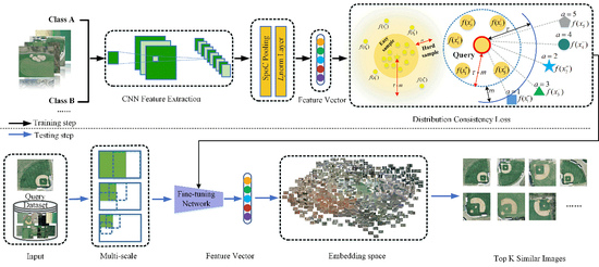
Figure 3.
An illustration of the proposed framework. At the top we train our network by the distribution consistency loss (DCL). The DCL consists of two parts: sample balance loss of positive samples and ranking consistency loss of negative samples. This loss established a valid feature representation by optimizing the distribution of hard and easy samples within the class, as well as the sorting of different types between classes. In the test phase, we input the image through multi-scale processing and input it into the fine-tuning network completed by the training phase, and then return the first K images associated with the query image.

Figure 4.
The flow diagram of our proposed distribution consistency loss.

Figure 5.
Sample images from the UCMD dataset.

Figure 6.
Sample images from the PatternNet dataset.

Figure 7.
Sample images from the NWPU-RESISC45 dataset.

Figure 8.
The impact of choice of the different τ selection. Performance on the evaluation of VGG16 (a) and ResNet50 (b) on PatternNet dataset. The curve line displays the evolution of mAP varying according to training epochs. Epoch the reflects off-the-shelf network.
Figure 8.
The impact of choice of the different τ selection. Performance on the evaluation of VGG16 (a) and ResNet50 (b) on PatternNet dataset. The curve line displays the evolution of mAP varying according to training epochs. Epoch the reflects off-the-shelf network.

Figure 9.
The impact of choice of the different m selection. Performance on the evaluation of VGG16 (a) and ResNet50 (b) on PatternNet dataset. The curve line displays the evolution of mAP varying according to training epochs. Epoch reflects the off-the-shelf network.
Figure 9.
The impact of choice of the different m selection. Performance on the evaluation of VGG16 (a) and ResNet50 (b) on PatternNet dataset. The curve line displays the evolution of mAP varying according to training epochs. Epoch reflects the off-the-shelf network.

Figure 10.
Performance (mAP) comparison of different pooling layers: max pooling, sum-pooling and generalized-mean pooling with the fine-tune VGG16 (a) and the fine-tune ResNet50 (b) on PatternNet.
Figure 10.
Performance (mAP) comparison of different pooling layers: max pooling, sum-pooling and generalized-mean pooling with the fine-tune VGG16 (a) and the fine-tune ResNet50 (b) on PatternNet.

Figure 11.
Category-level precision of different method under the VGG 16 network and ResNet 50 network on the UCMD dataset, PatternNet dataset and NWPU dataset. (a) VGG 16 + UCMD dataset, (b) ResNet 50 + UCMD dataset, (c) VGG 16 + PatternNet dataset, (d) ResNet 50 + PatternNet dataset, (e) VGG 16 + NWPU dataset, and (f) ResNet 50 + NWPU dataset. The category labels of the abscissa in the figure correspond one-to-one with the labels in Table 7, Table 8 and Table 9. Specifically, the labels of (a) and (b) correspond to Table 7, the labels of (c) and (d) correspond to Table 8, and corresponding to Table 9 are (e) and (f).


Figure 12.
Visualization of the proposed method with DCL on the UCMD dataset (up), PatternNet dataset (middle) and NWPU-RESISC45 dataset (down). Best viewed when zoomed in. Based on our approach, images with similar objects are more likely to be grouped together.
Figure 12.
Visualization of the proposed method with DCL on the UCMD dataset (up), PatternNet dataset (middle) and NWPU-RESISC45 dataset (down). Best viewed when zoomed in. Based on our approach, images with similar objects are more likely to be grouped together.


Table 1.
The impact of different τ on the distance distribution of negative examples. PatternNet is used. The mAP and Precision @ K (%) results are reported. Fine-tuned VGG16 produces a 512D vector and fine-tuned ResNet50 a 2048D vector.
Table 1.
The impact of different τ on the distance distribution of negative examples. PatternNet is used. The mAP and Precision @ K (%) results are reported. Fine-tuned VGG16 produces a 512D vector and fine-tuned ResNet50 a 2048D vector.
| Network | τ | P@5 | P@10 | P@50 | P@100 |
|---|---|---|---|---|---|
| VGG16 | 0.85 | 97.89 | 97.89 | 95.68 | 94.68 |
| 1.05 | 98.42 | 98.16 | 97.37 | 95.84 | |
| 1.25 | 97.37 | 97.32 | 96.05 | 94.43 | |
| 1.45 | 97.89 | 98.42 | 96.74 | 94.18 | |
| ResNet50 | 0.85 | 98.42 | 97.89 | 97.21 | 95.89 |
| 1.05 | 98.95 | 98.68 | 97.26 | 96.11 | |
| 1.25 | 99.47 | 99.21 | 98.53 | 98.08 | |
| 1.45 | 99.47 | 99.21 | 97.84 | 96.87 |
Table 2.
The impact of the distance margin m that be used to split positive and negative examples. The Precision @ K (%) results on PatternNet are displayed with τ = 1.05 in VGG16 and τ = 1.25 in ResNet50. Fine-tuned VGG16 produces a 512D vector and fine-tuned ResNet50 a 2048D vector.
Table 2.
The impact of the distance margin m that be used to split positive and negative examples. The Precision @ K (%) results on PatternNet are displayed with τ = 1.05 in VGG16 and τ = 1.25 in ResNet50. Fine-tuned VGG16 produces a 512D vector and fine-tuned ResNet50 a 2048D vector.
| Network | m | P@5 | P@10 | P@50 | P@100 |
|---|---|---|---|---|---|
| VGG16 | 0 | 98.42 | 97.63 | 95.11 | 93.21 |
| 0.2 | 98.95 | 98.42 | 98.16 | 98.00 | |
| 0.4 | 98.95 | 98.95 | 98.42 | 97.82 | |
| 0.6 | 98.22 | 98.22 | 98.69 | 98.35 | |
| 0.8 | 99.21 | 99.58 | 98.86 | 98.20 | |
| 1.0 | 99.47 | 99.74 | 99.11 | 98.34 | |
| ResNet50 | 0.2 | 100.00 | 99.74 | 99.21 | 98.82 |
| 0.4 | 98.95 | 98.95 | 98.42 | 97.82 | |
| 0.6 | 100.00 | 100.00 | 99.84 | 99.71 | |
| 0.8 | 98.98 | 99.47 | 99.79 | 99.58 | |
| 1.0 | 99.47 | 99.74 | 99.42 | 99.26 | |
| 1.2 | 100.00 | 100.00 | 99.89 | 99.81 |
Table 3.
Using the fine-tuned VGG16 to perform the evaluation of the multi-scale representation and ResNet50 with SPoC layer on PatternNet. Its original scale and down-sampled versions are represented together.
Table 3.
Using the fine-tuned VGG16 to perform the evaluation of the multi-scale representation and ResNet50 with SPoC layer on PatternNet. Its original scale and down-sampled versions are represented together.
| Pooling over Scales | Scale | mAP | P@5 | P@10 | P@50 | P@100 | ||||
|---|---|---|---|---|---|---|---|---|---|---|
| P@5 P@10 P@50 | ||||||||||
| VGG16 |  | 96.43 | 97.89 | 98.42 | 98.16 | 97.42 | ||||
| | | 98.05 | 98.95 | 99.21 | 99.32 | 98.95 | ||||
| | | | 94.66 | 98.95 | 97.89 | 97.21 | 96.05 | |||
| | | | | 94.09 | 98.42 | 97.89 | 96.84 | 95.66 | ||
| | | | | | 91.27 | 96.84 | 97.37 | 95.58 | 93.74 | |
| ResNet50 | | 99.38 | 100.00 | 99.74 | 99..95 | 99.68 | ||||
| | | 99.43 | 100.00 | 100.00 | 99.89 | 99.66 | ||||
| | | | 99.30 | 100.00 | 100.00 | 99.95 | 99.58 | |||
| | | | | 98.79 | 100.00 | 100.00 | 99.84 | 99.50 | ||
| | | | | | 97.96 | 100.00 | 100.00 | 99.74 | 98.61 | |
Table 4.
Comparison with state-of-the-art sampling methods. The network backbone is ResNet 50.
| Structural Loss | mAP | P@5 | P@10 | P@50 | P@100 | P@1000 |
|---|---|---|---|---|---|---|
| UCMD | ||||||
| Triplet Loss | 92.96 | 98.04 | 96.63 | 92.62 | 46.16 | 4.69 |
| N-pair-mc Loss | 91.81 | 94.04 | 91.46 | 90.49 | 45.08 | 4.67 |
| Proxy NCA Loss | 95.72 | 97.98 | 96.65 | 94.23 | 47.02 | 4.71 |
| Lifted Struct Loss | 96.08 | 98.90 | 97.82 | 95.78 | 47.46 | 4.76 |
| DSLL | 97.34 | 98.98 | 98.42 | 96.93 | 48.67 | 4.86 |
| Our DCL | 98.76 | 100.00 | 100.00 | 99.33 | 49.82 | 5.21 |
| PatternNet | ||||||
| Triplet Loss | 94.94 | 99.52 | 97.92 | 96.13 | 95.07 | 15.61 |
| N-pair-mc Loss | 94.11 | 97.94 | 95.15 | 94.33 | 98.17 | 15.52 |
| Proxy NCA Loss | 97.71 | 98.56 | 98.69 | 98.89 | 98.45 | 15.74 |
| Lifted Struct Loss | 98.58 | 98.05 | 98.62 | 98.75 | 98.88 | 15.79 |
| DSLL | 98.52 | 99.09 | 98.03 | 96.68 | 98.69 | 15.83 |
| Our DCL | 99.43 | 100.00 | 100.00 | 99.89 | 99.66 | 16.38 |
| NWPU-RESISC45 | ||||||
| Triplet Loss | 93.82 | 98.65 | 96.85 | 96.07 | 94.83 | 15.34 |
| N-pair-mc Loss | 93.06 | 97.86 | 95.12 | 94.35 | 98.15 | 15.46 |
| Proxy NCA Loss | 97.68 | 97.54 | 97.57 | 97.91 | 97.44 | 15.69 |
| Lifted Struct Loss | 97.47 | 97.03 | 97.42 | 97.63 | 97.72 | 15.76 |
| DSLL | 98.54 | 99.05 | 98.15 | 96.34 | 98.45 | 15.78 |
| Our DCL | 99.44 | 100.00 | 100.00 | 99.91 | 99.70 | 16.42 |
Table 5.
Retrieval precision of different positive sample numbers for the PatternNet dataset after training the ResNet50 network.
Table 5.
Retrieval precision of different positive sample numbers for the PatternNet dataset after training the ResNet50 network.
| Number (n) | Weights | mAP |
|---|---|---|
| 1 | 1 | 95.85 |
| 5 | 1 | 93.21 |
| 5 | 1/n | 94.93 |
| 5 | Dynamic | 97.48 |
| 10 | 1 | 90.15 |
| 10 | 1/n | 93.85 |
| 10 | Dynamic | 95.32 |
Table 6.
Retrieval precision of different negative sample numbers for the PatternNet dataset after training the ResNet50 network.
Table 6.
Retrieval precision of different negative sample numbers for the PatternNet dataset after training the ResNet50 network.
| Number | Category Restrictions | mAP |
|---|---|---|
| 5 | yes | 97.48 |
| 5 | no | 95.16 |
| 10 | yes | 94.52 |
| 10 | no | 92.14 |
| 15 | yes | 93.42 |
| 15 | no | 91.35 |
Table 7.
Retrieval precision of each individual category for the UCMD dataset after training the VGG16 and ResNet50 network.
Table 7.
Retrieval precision of each individual category for the UCMD dataset after training the VGG16 and ResNet50 network.
| Categories | VGG16 | ResNet50 | ||
|---|---|---|---|---|
| Pretrained | DCL | Pretrained CNNs | DCL | |
| Agriculture (1) | 0.94 | 1.00 | 0.99 | 1.00 |
| Airplane (2) | 0.66 | 1.00 | 0.99 | 1.00 |
| Baseball diamond (3) | 0.60 | 0.99 | 0.59 | 1.00 |
| Beach (4) | 0.99 | 1.00 | 0.99 | 1.00 |
| Buildings (5) | 0.33 | 0.74 | 0.37 | 0.99 |
| Chaparral (6) | 0.99 | 1.00 | 1.00 | 1.00 |
| Dense residential (7) | 0.36 | 0.94 | 0.24 | 0.97 |
| Forest (8) | 0.88 | 1.00 | 0.99 | 1.00 |
| Freeway (9) | 0.55 | 0.99 | 0.87 | 0.99 |
| Golf course (10) | 0.42 | 0.99 | 0.83 | 1.00 |
| Harbor (11) | 0.59 | 1.00 | 0.68 | 1.00 |
| Intersection (12) | 0.31 | 0.98 | 0.31 | 0.98 |
| Medium residential (13) | 0.48 | 0.93 | 0.61 | 0.99 |
| Mobile home park (14) | 0.58 | 1.00 | 0.72 | 1.00 |
| Overpass (15) | 0.37 | 0.97 | 0.51 | 0.99 |
| Parking lot (16) | 0.79 | 1.00 | 0.32 | 0.83 |
| River (17) | 0.67 | 0.98 | 0.60 | 0.99 |
| Runway (18) | 0.57 | 1.00 | 0.89 | 1.00 |
| Sparse residential (19) | 0.11 | 0.89 | 0.55 | 0.99 |
| Storage tanks (20) | 0.77 | 0.99 | 0.88 | 1.00 |
| Tennis court (21) | 0.39 | 1.00 | 0.78 | 1.00 |
Table 8.
Retrieval precision of each individual category for the PatternNet dataset after training the VGG16 and ResNet50 network.
Table 8.
Retrieval precision of each individual category for the PatternNet dataset after training the VGG16 and ResNet50 network.
| Categories | VGG16 | ResNet50 | ||
|---|---|---|---|---|
| Pretrained | DCL | Pretrained CNNs | DCL | |
| Airplane (1) | 0.95 | 1.00 | 0.92 | 1.00 |
| Baseball field (2) | 0.97 | 0.99 | 0.96 | 1.00 |
| Basketball court (3) | 0.50 | 0.97 | 0.45 | 0.98 |
| Beach (4) | 1.00 | 1.00 | 0.99 | 1.00 |
| Bridge (5) | 0.24 | 0.98 | 0.13 | 0.99 |
| Cemetery (6) | 0.93 | 1.00 | 0.93 | 1.00 |
| Chaparral (7) | 0.99 | 1.00 | 1.00 | 1.00 |
| Christmas tree farm (8) | 0.98 | 1.00 | 0.83 | 1.00 |
| Closed road (9) | 0.93 | 0.99 | 0.91 | 0.99 |
| Coastal mansion (10) | 0.99 | 0.97 | 0.98 | 0.99 |
| Crosswalk (11) | 0.96 | 1.00 | 0.93 | 1.00 |
| Dense residential (12) | 0.52 | 0.82 | 0.46 | 0.99 |
| Ferry terminal (13) | 0.58 | 0.83 | 0.40 | 0.87 |
| Football field (14) | 0.97 | 0.99 | 0.89 | 1.00 |
| Forest (15) | 0.99 | 1.00 | 1.00 | 1.00 |
| Freeway (16) | 0.99 | 1.00 | 0.99 | 1.00 |
| Golf course (17) | 0.95 | 0.99 | 0.95 | 0.99 |
| Harbor (18) | 0.89 | 0.96 | 0.92 | 0.96 |
| Intersection (19) | 0.52 | 0.98 | 0.51 | 0.99 |
| Mobile home park (20) | 0.86 | 0.99 | 0.81 | 1.00 |
| Nursing home (21) | 0.23 | 0.96 | 0.59 | 0.98 |
| Oil gas field (22) | 0.99 | 1.00 | 0.99 | 1.00 |
| Oilwell (23) | 1.00 | 1.00 | 1.00 | 1.00 |
| Overpass (24) | 0.77 | 0.99 | 0.90 | 0.99 |
| Parking lot (24) | 0.99 | 0.99 | 0.98 | 1.00 |
| Parking space (26) | 0.52 | 1.00 | 0.47 | 1.00 |
| Railway (27) | 0.83 | 0.99 | 0.78 | 1.00 |
| River (28) | 0.99 | 1.00 | 0.99 | 1.00 |
| Runway (29) | 0.29 | 0.99 | 0.36 | 0.99 |
| Runway marking (30) | 0.99 | 0.99 | 0.99 | 1.00 |
| Shipping yard (31) | 0.97 | 0.99 | 0.99 | 0.99 |
| Solar panel (32) | 0.99 | 0.99 | 0.99 | 1.00 |
| Sparse residential (33) | 0.64 | 0.91 | 0.47 | 0.99 |
| Storage tank (34) | 0.42 | 0.99 | 0.55 | 0.99 |
| Swimming pool (35) | 0.18 | 0.96 | 0.43 | 0.99 |
| Tennis court (36) | 0.59 | 0.91 | 0.31 | 0.97 |
| Transformer station (37) | 0.69 | 0.99 | 0.63 | 0.99 |
| Wastewater plant (38) | 0.91 | 0.98 | 0.90 | 0.99 |
Table 9.
Retrieval precision of each individual category for the NWPU-RESISC45 dataset after training the VGG16 and ResNet50 network.
Table 9.
Retrieval precision of each individual category for the NWPU-RESISC45 dataset after training the VGG16 and ResNet50 network.
| Categories | VGG16 | ResNet50 | ||
|---|---|---|---|---|
| Pretrained | DCL | Pretrained CNNs | DCL | |
| Airplane (1) | 0.76 | 1.00 | 0.88 | 1.00 |
| Airport (2) | 0.66 | 0.97 | 0.72 | 1.00 |
| Baseball Diamond (3) | 0.64 | 0.97 | 0.69 | 0.99 |
| Basketball Court (4) | 0.51 | 0.95 | 0.60 | 0.98 |
| Beach (5) | 0.77 | 1.00 | 0.76 | 1.00 |
| Bridge (6) | 0.85 | 1.00 | 0.72 | 1.00 |
| Chaparral (7) | 1.00 | 1.00 | 1.00 | 1.00 |
| Church (8) | 0.55 | 0.97 | 0.56 | 0.97 |
| Circular Farmland (9) | 0.93 | 1.00 | 0.96 | 1.00 |
| Cloud (10) | 0.89 | 1.00 | 0.91 | 1.00 |
| Commercial Area (11) | 0.64 | 0.99 | 0.81 | 1.00 |
| Dense residential (12) | 0.77 | 1.00 | 0.88 | 1.00 |
| Desert (13) | 0.84 | 1.00 | 0.86 | 1.00 |
| Forest (14) | 1.00 | 1.00 | 0.94 | 1.00 |
| Freeway (15) | 0.71 | 0.92 | 0.62 | 0.98 |
| Golf course (16) | 0.79 | 0.99 | 0.95 | 1.00 |
| Ground Track Field (17) | 0.80 | 0.97 | 0.62 | 0.98 |
| Harbor (18) | 0.84 | 1.00 | 0.92 | 1.00 |
| Industrial Area (19) | 0.71 | 0.98 | 0.76 | 0.99 |
| Intersection (20) | 0.70 | 0.95 | 0.63 | 0.98 |
| Island (21) | 1.00 | 1.00 | 1.00 | 1.00 |
| Lake (22) | 0.88 | 1.00 | 0.80 | 1.00 |
| Meadow (23) | 0.82 | 1.00 | 0.84 | 1.00 |
| Medium Residential (24) | 0.70 | 0.99 | 0.78 | 1.00 |
| Mobile Home Park (25) | 0.71 | 1.00 | 0.92 | 1.00 |
| Mountain (26) | 0.86 | 1.00 | 0.87 | 1.00 |
| Overpass (27) | 0.72 | 0.99 | 0.86 | 1.00 |
| Palace (28) | 0.52 | 0.94 | 0.40 | 0.98 |
| Parking Lot (29) | 0.87 | 1.00 | 1.00 | 1.00 |
| Railway (30) | 0.77 | 1.00 | 0.89 | 1.00 |
| Railway Station (31) | 0.65 | 0.95 | 0.63 | 0.98 |
| Rectangular Farmland (32) | 0.85 | 1.00 | 0.83 | 0.99 |
| River (33) | 0.69 | 0.98 | 0.69 | 0.99 |
| Roundabout (34) | 0.80 | 1.00 | 0.71 | 1.00 |
| Runway (35) | 0.77 | 1.00 | 0.78 | 1.00 |
| Sea Ice (36) | 1.00 | 1.00 | 1.00 | 1.00 |
| Ship (37) | 0.65 | 0.91 | 0.60 | 0.98 |
| Snowberg (38) | 0.95 | 1.00 | 0.96 | 1.00 |
| Sparse Residential (39) | 0.81 | 1.00 | 0.68 | 0.98 |
| Stadium (40) | 0.76 | 1.00 | 0.80 | 1.00 |
| Storage Tank (41) | 0.81 | 1.00 | 0.87 | 1.00 |
| Tennis Court (42) | 0.56 | 0.99 | 0.81 | 1.00 |
| Terrace (43) | 0.73 | 1.00 | 0.87 | 1.00 |
| Thermal Power Station (44) | 0.64 | 0.98 | 0.66 | 0.98 |
| Wetland (45) | 0.68 | 0.98 | 0.83 | 1.00 |
Table 10.
mAP (%) and P@ (%) on the UCMD dataset comparing with the state-of-the-art methods.
| Features | mAP | P@5 | P@10 | P@50 | P@100 | P@1000 |
|---|---|---|---|---|---|---|
| RAN-KNN [46] | 26.74 | - | 24.90 | - | - | - |
| GoogLeNet [46] | 53.13 | - | 80.96 | - | - | - |
| VGG-VD19 [46] | 53.19 | - | 77.60 | - | - | - |
| VGG-VD16 [46] | 53.71 | - | 78.34 | - | - | - |
| KSLSH [32] | 63.00 | - | - | - | - | - |
| GCN [46] | 64.81 | - | 87.12 | - | - | - |
| SGCN [46] | 69.89 | - | 93.63 | - | - | - |
| VGG16 [27] | 81.30 | 89.50 | 87.60 | 78.30 | - | - |
| ResNet50 [27] | 84.00 | 91.90 | 91.40 | 84.50 | - | - |
| MiLaN [34] | 90.40 | - | - | - | - | - |
| FC6 (VGG16) [47] | 91.65 | - | - | - | - | - |
| FC7 (VGG16) [47] | 92.00 | - | - | - | - | - |
| Pool5 (ResNet50) [47] | 95.62 | - | - | - | - | - |
| Ours (VGG16) | 97.34 | 97.14 | 97.62 | 98.67 | 48.95 | 3.98 |
| Ours (ResNet50) | 98.76 | 100.00 | 100.00 | 99.33 | 49.82 | 5.21 |
Table 11.
mAP (%) and P@ (%) on the PatternNet dataset comparing with the state-of-the-art methods.
| Features | mAP | P@5 | P@10 | P@50 | P@100 | P@1000 |
|---|---|---|---|---|---|---|
| G-KNN [46] | 12.35 | - | 13.24 | - | - | - |
| RAN-KNN [46] | 22.56 | - | 37.70 | - | - | - |
| UFL [9] | 25.35 | 52.09 | 48.82 | 38.11 | 31.92 | 9.79 |
| Gabor Texture [9] | 27.73 | 68.55 | 62.78 | 44.61 | 35.52 | 8.99 |
| VLAD [9] | 34.10 | 58.25 | 55.70 | 47.57 | 41.11 | 11.04 |
| VGG-VD19 [46] | 57.89 | - | 91.13 | - | - | - |
| VGG-VD16 [46] | 59.86 | - | 92.04 | - | - | - |
| VGGF Fc1 [9] | 61.95 | 92.46 | 90.37 | 79.26 | 69.05 | 14.25 |
| GoogLeNet [46] | 63.11 | - | 93.31 | - | - | - |
| VGGF Fc2 [9] | 63.37 | 91.52 | 89.64 | 79.99 | 70.47 | 14.52 |
| VGGS Fc1 [9] | 63.28 | 92.74 | 90.70 | 80.03 | 70.13 | 14.36 |
| VGGS Fc2 [9] | 63.74 | 91.92 | 90.09 | 80.31 | 70.73 | 14.55 |
| ResNet50 [9] | 68.23 | 94.13 | 92.41 | 83.71 | 74.93 | 14.64 |
| LDCNN [9] | 69.17 | 66.81 | 66.11 | 67.47 | 68.80 | 14.08 |
| SGCN [46] | 71.79 | - | 97.14 | - | - | - |
| GCN [46] | 73.11 | - | 95.53 | - | - | - |
| FC6 (VGG16) [47] | 96.21 | - | - | - | - | - |
| FC7 (VGG16) [47] | 96.48 | - | - | - | - | - |
| Pool5 (ResNet50) [47] | 98.49 | - | - | - | - | - |
| Ours (VGG16) | 98.05 | 98.95 | 99.21 | 99.32 | 98.95 | 15.47 |
| Ours (ResNet50) | 99.43 | 100.00 | 100.00 | 99.89 | 99.66 | 16.38 |
© 2020 by the authors. Licensee MDPI, Basel, Switzerland. This article is an open access article distributed under the terms and conditions of the Creative Commons Attribution (CC BY) license (http://creativecommons.org/licenses/by/4.0/).
Share and Cite
MDPI and ACS Style
Fan, L.; Zhao, H.; Zhao, H. Distribution Consistency Loss for Large-Scale Remote Sensing Image Retrieval. Remote Sens. 2020, 12, 175. https://doi.org/10.3390/rs12010175
AMA Style
Fan L, Zhao H, Zhao H. Distribution Consistency Loss for Large-Scale Remote Sensing Image Retrieval. Remote Sensing. 2020; 12(1):175. https://doi.org/10.3390/rs12010175
Chicago/Turabian StyleFan, Lili, Hongwei Zhao, and Haoyu Zhao. 2020. "Distribution Consistency Loss for Large-Scale Remote Sensing Image Retrieval" Remote Sensing 12, no. 1: 175. https://doi.org/10.3390/rs12010175
Note that from the first issue of 2016, this journal uses article numbers instead of page numbers. See further details here.