A System for Weeds and Crops Identification—Reaching over 10 FPS on Raspberry Pi with the Usage of MobileNets, DenseNet and Custom Modifications


Abstract
:1. Introduction
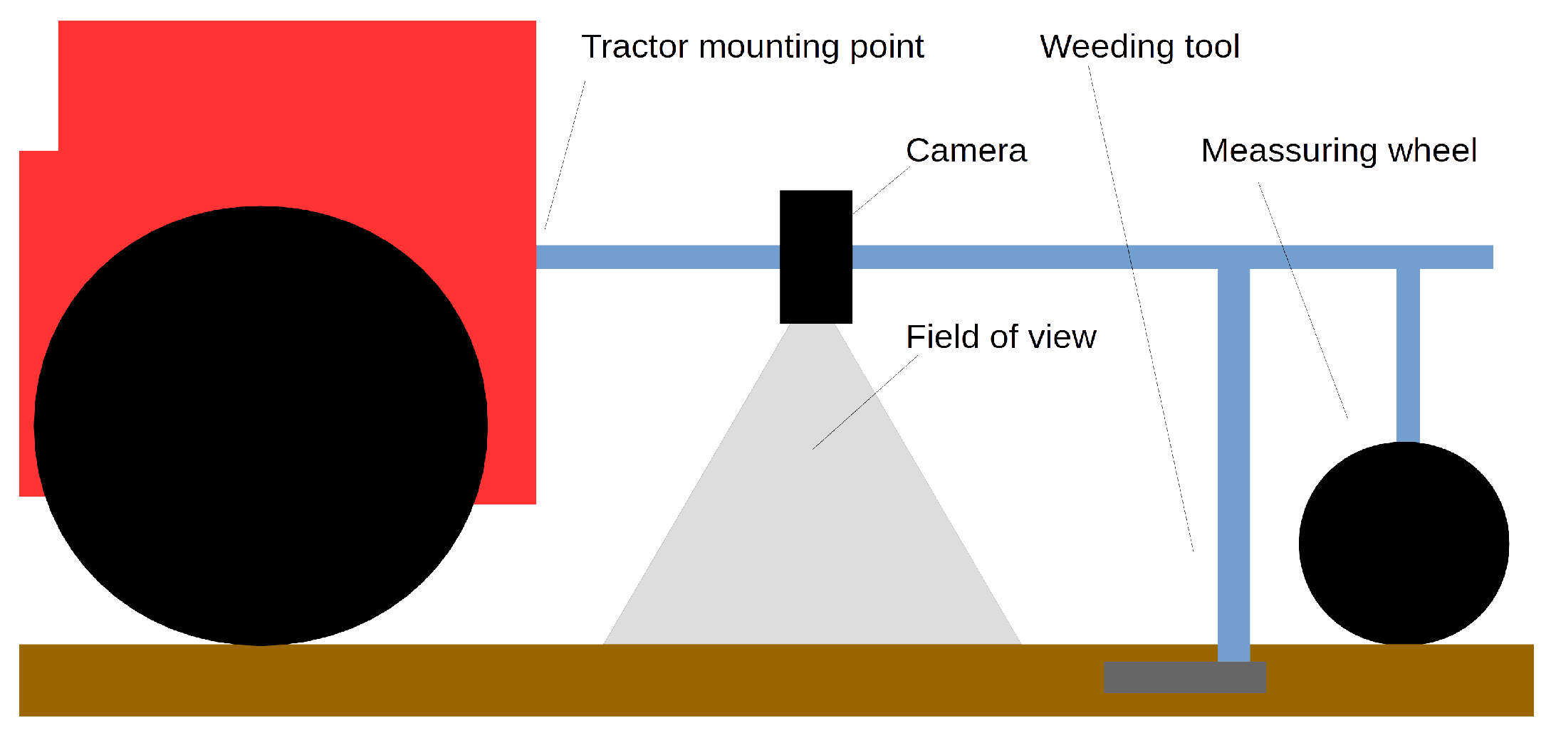
2. Overview of the Weeding Machine
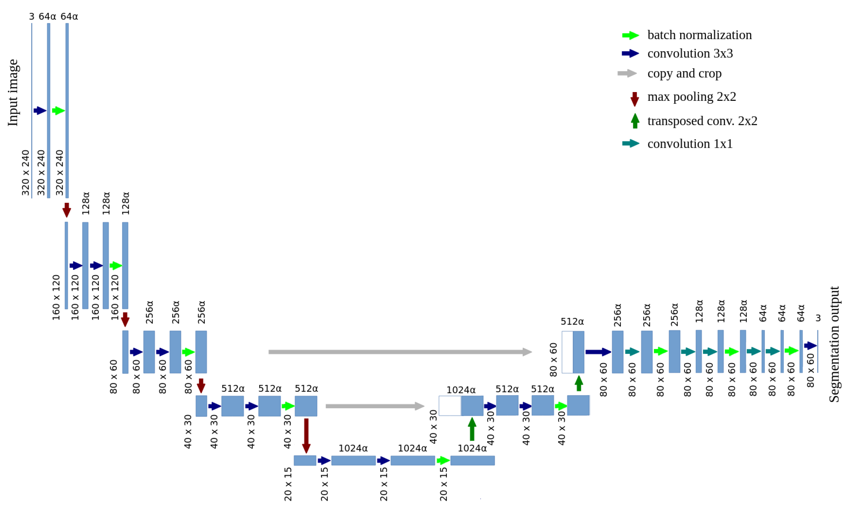
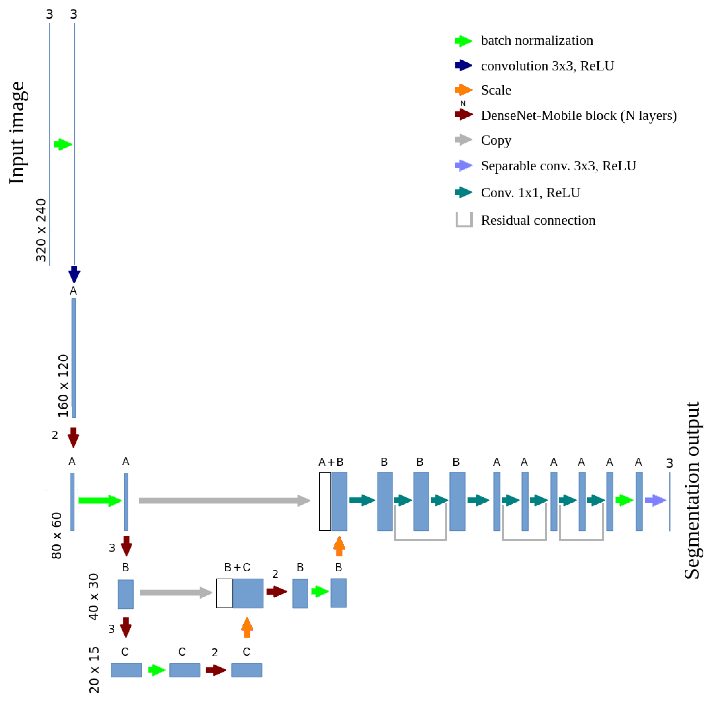
3. Development Methodology of the Plant Segmentation System
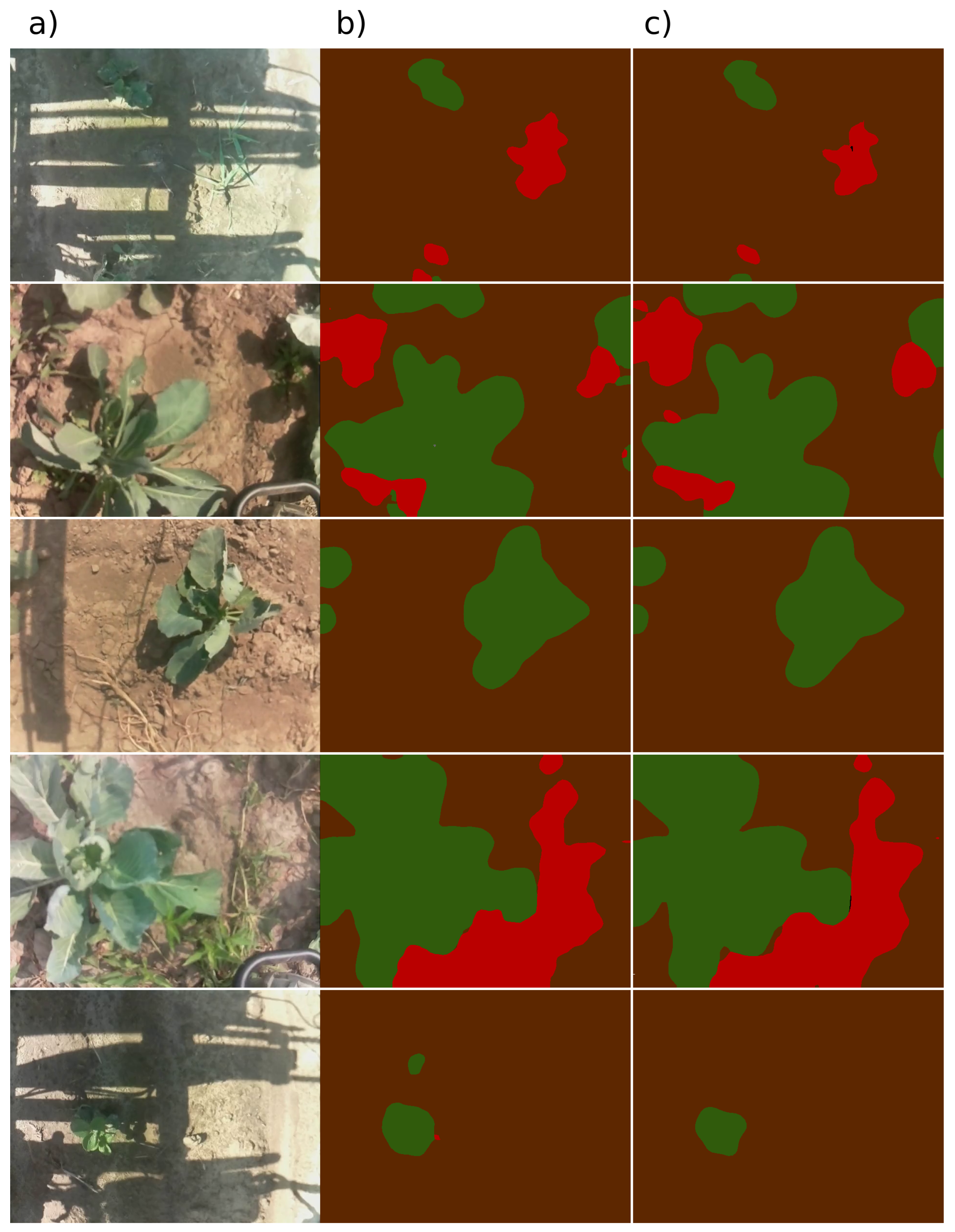
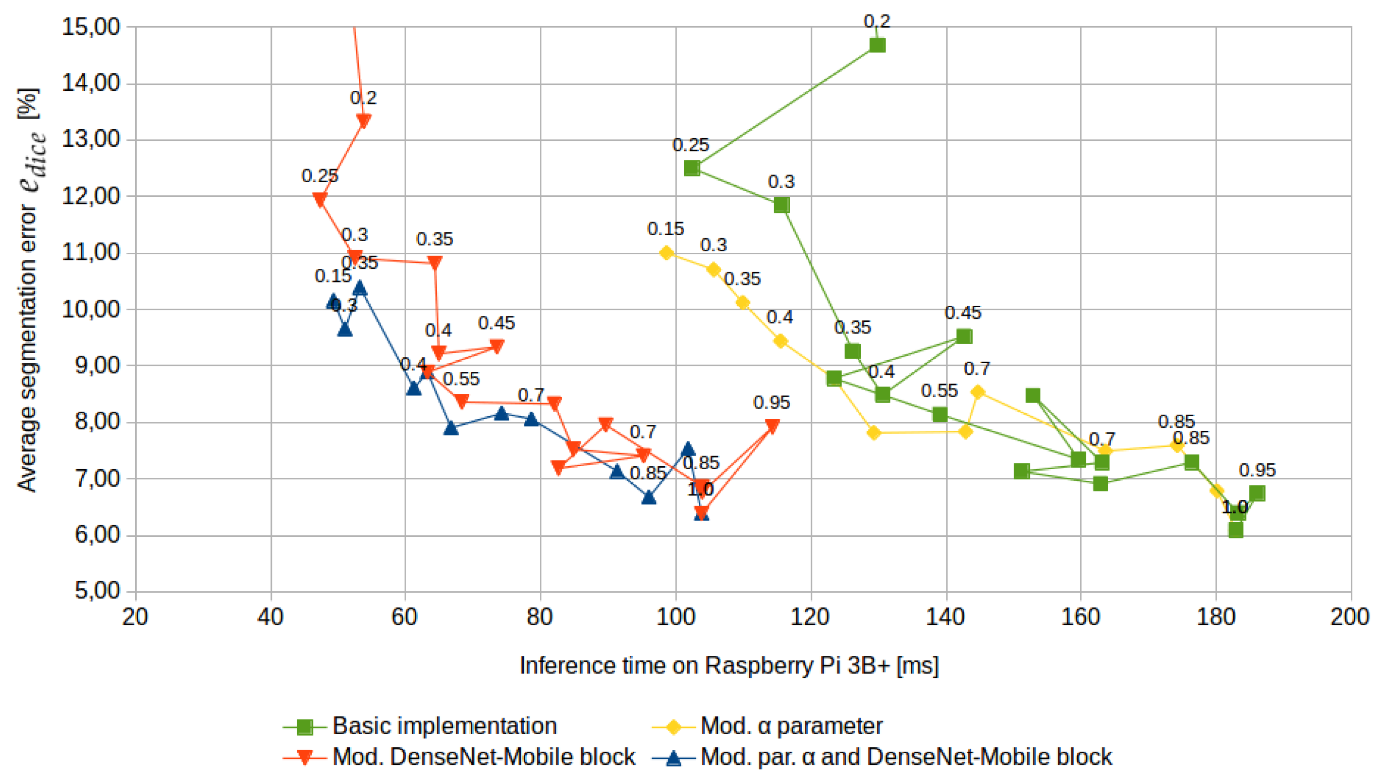
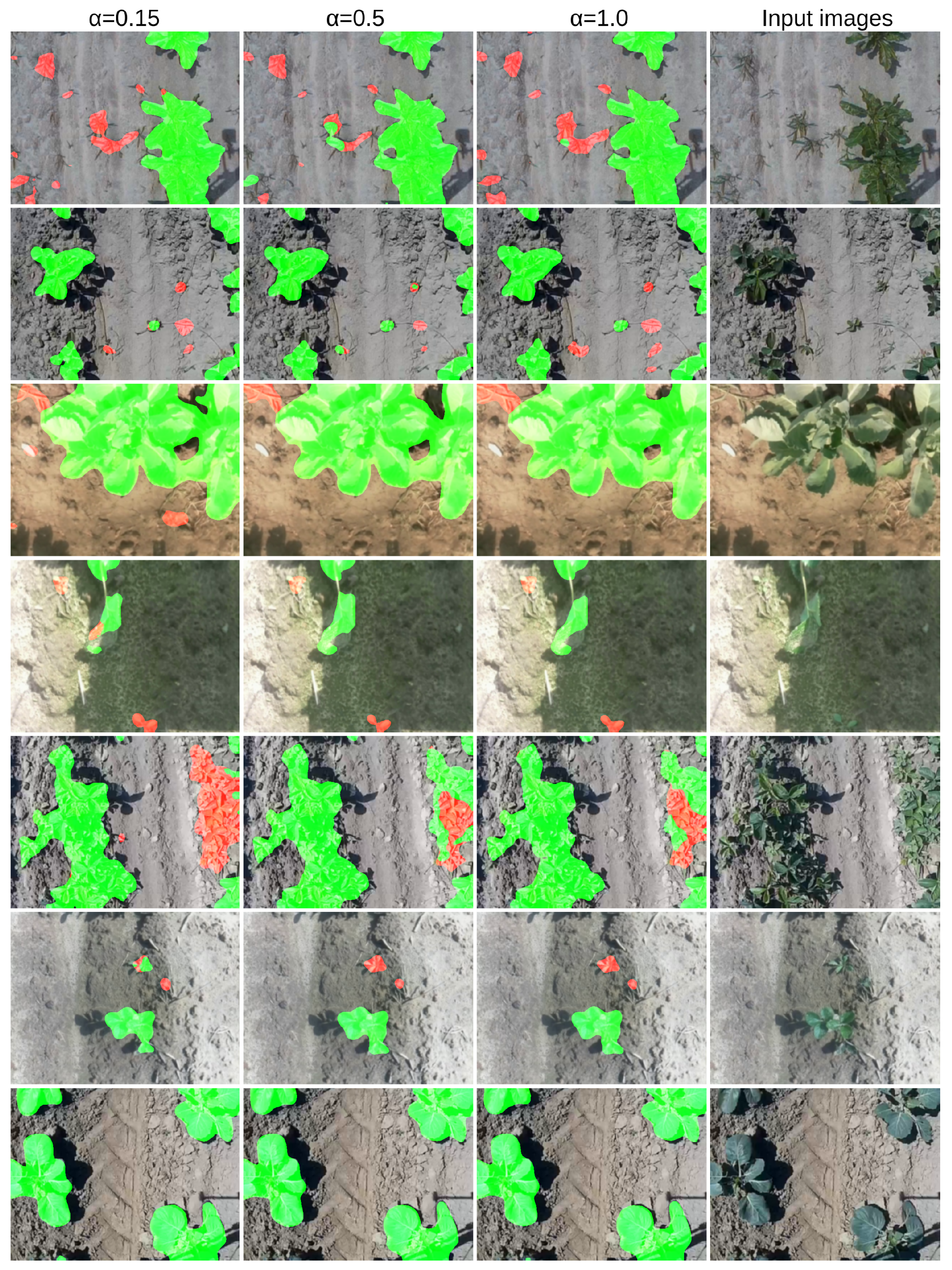
4. Experimental Results
5. Conclusions
- Training of different models for different plant species and growth stadiums.
- Change of the parameter value.
- Change of the number of final residual layers.
- Reduction of the number of batch normalization operations.
Author Contributions
Funding
Conflicts of Interest
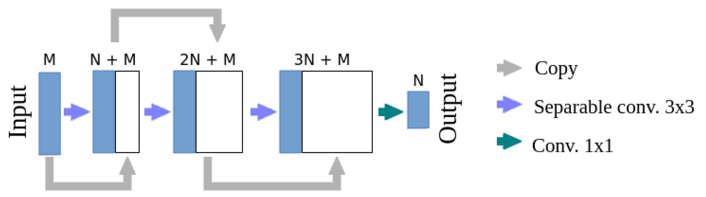
Appendix A
Appendix A.1.
def densenetmobile_naive(input, num_filters, layers, stride=1,
                          activation=tf.nn.relu):
    prev_cat = input
    for i in range(layers + 1):
      conv = tf.layers.separable_conv2d(prev_cat, filters=num_filters,
           kernel_size=3, strides=1, activation=activation,
           padding=’same’,
           depthwise_initializer=tf.initializers.he_normal(),
           pointwise_initializer=tf.initializers.he_normal())
      prev_cat = tf.concat((prev_cat, conv), −1)
    conv_bottleneck = tf.layers.conv2d(prev_cat, filters=num_filters,
      kernel_size=1, strides=stride, activation=None, padding=‘same’,
      kernel_initializer=tf.initializers.he_normal())
    return conv_bottleneck
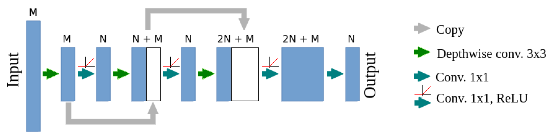
Appendix A.2.
def densenetmobile_modified(input, num_filters, layers, stride=1,
				activation=tf.nn.relu, name=’layer_name’):
	strides = [1, stride, stride, 1]
	filters_input = tf.get_variable(name + ’depthinput/kernel’,
				[3, 3, input.shape[−1], 1],
				tf.float32, tf.initializers.he_normal())
	conv_depth_input = tf.nn.depthwise_conv2d(input, filter=filters_input,
					strides=strides, padding=’SAME’,
					name=name+’depthinput’)
	concated_depth = conv_depth_input
	for i in range(layers):
		letter = chr(ord(’A’) + i)
		conv_1x1 = tf.layers.conv2d(concated_depth, filters=num_filters,
				kernel_size=1, strides=1, activation=activation,
				padding=’same’, name=name + ’_1x1_’ + letter,
				kernel_initializer=tf.initializers.he_normal())
		filters = tf.get_variable(name + ’_depth_’ + letter + ’/kernel’,
				[3, 3, num_filters, 1], tf.float32,
				tf.initializers.he_normal())
		conv_depth = tf.nn.depthwise_conv2d(conv_1x1, filter=filters,
				strides=[1, 1, 1, 1], padding=’SAME’,
				name=name + letter)
		concated_depth = tf.concat((concated_depth, conv_depth), −1)
	conv_block = tf.layers.conv2d(concated_depth, filters=layers * \
				num_filters, kernel_size=1, strides=1,
				activation=activation, padding=’same’,
				name=name + ’_block’,
				kernel_initializer=tf.initializers.he_normal())
	conv_bottleneck = tf.layers.conv2d(conv_block, filters=num_filters,
				kernel_size=1, strides=1, activation=None,
				padding=’same’, name=name + ’_bottleneck’,
				kernel_initializer=tf.initializers.he_normal())
	return conv_bottleneck
References
- Chechliński, Ł.; Siemiątkowska, B.; Majewski, M. A System for Weeds and Crops Identification Based on Convolutional Neural Network. In Conference on Automation; Springer: Cham, Switzerland, 2018; pp. 193–202. [Google Scholar]
- Sardana, V.; Mahajan, G.; Jabran, K.; Chauhan, B.S. Role of competition in managing weeds: An introduction to the special issue. Crop. Prot. 2017, 95, 1–7. [Google Scholar] [CrossRef]
- Mystkowska, I.; Zarzecka, K.; Baranowska, A.; Gugała, M. An effect of herbicides and their mixtures on potato yielding and efficacy in potato crop. Prog. Plant Prot. 2017, 57, 21–26. [Google Scholar]
- Sujaritha, M.; Lakshminarasimhan, M.; Fernandez, C.J.; Chandran, M. Greenbot: A solar autonomous robot to uproot weeds in a grape field. Int. J. Comput. Sci. Eng. 2016, 4, 1351–1358. [Google Scholar]
- Keresztes, B.; Grenier, G.; Germain, C.; Da Costa, J.-P.; Beaulieu, X.D. VVINNER: An autonomous robot for automated scoring of vineyards. In Proceedings of the International Conference of Agricultural Engineering, Zurich, Switzerland, 6–10 July 2014. [Google Scholar]
- Malavazi, F.B.; Guyonneau, R.; Fasquel, J.B.; Lagrange, S.; Mercier, F. LiDAR-only based navigation algorithm for an autonomous agricultural robot. Comput. Electron. Agric. 2018, 154, 71–79. [Google Scholar] [CrossRef]
- Nørremark, M.; Griepentrog, H.W.; Nielsen, J.; Søgaard, H.T. Evaluation of an autonomous GPS-based system for intra-row weed control by assessing the tilled area. Precis. Agric. 2012, 13, 149–162. [Google Scholar] [CrossRef]
- Wäldchen, J.; Mäder, P. Plant Species Identification Using Computer Vision Techniques: A Systematic Literature Review. Arch. Comput. Methods Eng. 2017, 25, 507–543. [Google Scholar] [CrossRef] [PubMed] [Green Version]
- Priyankara, H.A.C.; Withanage, D.K. Computer assisted plant identification system for Android. In Proceedings of the 2015 Moratuwa Engineering Research Conference (MERCon), Moratuwa, Sri Lanka, 7–8 April 2015; pp. 148–153. [Google Scholar] [CrossRef]
- Lowe, D.G. Object Recognition from Local Scale-Invariant Features. In Proceedings of the ICCV ’99 International Conference on Computer Vision, Kerkyra, Greece, 20–27 September 1999; IEEE Computer Society: Washington, DC, USA, 1999; Volume 2, p. 1150. [Google Scholar]
- Beghin, T.; Cope, J.S.; Remagnino, P.; Barman, S. Shape and Texture Based Plant Leaf Classification. In Proceedings of the Advanced Concepts for Intelligent Vision Systems: 12th International Conference (ACIVS 2010), Sydney, Australia, 13–16 December 2010, Part II; Springer: Berlin/Heidelberg, Germany, 2010; pp. 345–353. [Google Scholar] [CrossRef]
- Wu, S.G.; Bao, F.S.; Xu, E.Y.; Wang, Y.X.; Chang, Y.F.; Xiang, Q.L. A Leaf Recognition Algorithm for Plant Classification Using Probabilistic Neural Network. In Proceedings of the IEEE international symposium on signal processing and information technology, Cairo, Egypt, 15–18 December 2007; pp. 11–16. [Google Scholar]
- Tsolakidis, D.G.; Kosmopoulos, D.I.; Papadourakis, G. Plant Leaf Recognition Using Zernike Moments and Histogram of Oriented Gradients. In Proceedings of the Artificial Intelligence: Methods and Applications: 8th Hellenic Conference on AI (SETN 2014), Ioannina, Greece, 15–17 May 2014; Springer International Publishing: Cham, Switzerland, 2014; pp. 406–417. [Google Scholar] [CrossRef]
- Caglayan, A.; Guclu, O.; Can, A.B. A Plant Recognition Approach Using Shape and Color Features in Leaf Images. In Proceedings of the Image Analysis and Processing—ICIAP 2013: 17th International Conference, Naples, Italy, 9–13 September 2013, Part II; Springer: Berlin/Heidelberg, Germany, 2013; pp. 161–170. [Google Scholar] [CrossRef] [Green Version]
- Yanikoglu, B.; Aptoula, E.; Tirkaz, C. Automatic Plant Identification from Photographs. Mach. Vision Appl. 2014, 25, 1369–1383. [Google Scholar] [CrossRef]
- Zhang, J.; He, L.; Karkee, M.; Zhang, Q.; Zhang, X.; Gao, Z. Branch detection for apple trees trained in fruiting wall architecture using depth features and Regions-Convolutional Neural Network (R-CNN). Comput. Electron. Agric. 2018, 155, 386–393. [Google Scholar] [CrossRef]
- Kamilaris, A.; Prenafeta-Boldú, F.X. Deep learning in agriculture: A survey. Comput. Electron. Agric. 2018, 147, 70–90. [Google Scholar] [CrossRef] [Green Version]
- Kamilaris, A.; Prenafeta-Boldú, F. A review of the use of convolutional neural networks in agriculture. J. Agric. Sci. 2018, 156, 312–322. [Google Scholar] [CrossRef] [Green Version]
- Howard, A.G.; Zhu, M.; Chen, B.; Kalenichenko, D.; Wang, W.; Weyand, T.; Andreetto, M.; Adam, H. Mobilenets: Efficient convolutional neural networks for mobile vision applications. arXiv 2017, arXiv:1704.04861. [Google Scholar]
- He, K.; Zhang, X.; Ren, S.; Sun, J. Deep residual learning for image recognition. In Proceedings of the IEEE Conference on Computer Vision and Pattern Recognition, Las Vegas, NV, USA, 27–30 June 2016; pp. 770–778. [Google Scholar]
- Huang, G.; Liu, Z.; Van Der Maaten, L.; Weinberger, K.Q. Densely connected convolutional networks. In Proceedings of the IEEE Conference on Computer Vision and Pattern Recognition, Honolulu, HI, USA, 21–26 July 2017; pp. 4700–4708. [Google Scholar]
- Ronneberger, O.; Fischer, P.; Brox, T. U-net: Convolutional networks for biomedical image segmentation. In Proceedings of the International Conference on Medical Image Computing and Computer-Assisted Intervention, Munich, Germany, 5–9 October 2015; Springer: Cham, Switzerland, 2015; pp. 234–241. [Google Scholar]
- Zhao, H.; Shi, J.; Qi, X.; Wang, X.; Jia, J. Pyramid scene parsing network. In Proceedings of the IEEE Conference on Computer Vision and Pattern Recognition, Honolulu, HI, USA, 21–26 July 2017; pp. 2881–2890. [Google Scholar]
- Olsen, A.; Konovalov, D.A.; Philippa, B.; Ridd, P.; Wood, J.C.; Johns, J.; Banks, W.; Girgenti, B.; Kenny, O.; Whinney, J.; et al. DeepWeeds: A multiclass weed species image dataset for deep learning. Sci. Rep. 2019, 9, 2058. [Google Scholar] [CrossRef] [PubMed]
- Chavan, T.R.; Nandedkar, A.V. AgroAVNET for crops and weeds classification: A step forward in automatic farming. Comput. Electron. Agric. 2018, 154, 361–372. [Google Scholar] [CrossRef]
- Sa, I.; Ge, Z.; Dayoub, F.; Upcroft, B.; Perez, T.; McCool, C. Deepfruits: A fruit detection system using deep neural networks. Sensors 2016, 16, 1222. [Google Scholar] [CrossRef] [PubMed]
- Rahnemoonfar, M.; Sheppard, C. Deep count: Fruit counting based on deep simulated learning. Sensors 2017, 17, 905. [Google Scholar] [CrossRef] [PubMed]
- Dietenbeck, T.; Alessandrini, M.; Friboulet, D.; Bernard, O. CREASEG: a free software for the evaluation of image segmentation algorithms based on level-set. In Proceedings of the 2010 IEEE International Conference on Image Processing, Hong Kong, China, 26–29 September 2010; pp. 665–668. [Google Scholar]


| Configuration | [%] | [%] | [%] | [%] |
|---|---|---|---|---|
| Single model—average results | 3.55 | 53.8 | 60.2 | 1.0 |
| Ensemble of 50 instances—mean | 1.68 | 72.9 | 66.3 | 0.2 |
| Ensemble of 50 instances—media | 1.71 | 74.0 | 65.0 | 0.2 |
| [%] | [%] | [%] | [%] | |
|---|---|---|---|---|
| 0.15 | 2.66 | 67.2 | 50.5 | 0.9 |
| 0.3 | 2.49 | 70.7 | 54.7 | 0.2 |
| 0.35 | 2.28 | 79.3 | 47.4 | 0.2 |
| 0.4 | 2.32 | 76.8 | 57.1 | 0.3 |
| 0.5 | 2.07 | 77.9 | 55.0 | 0.2 |
| 0.6 | 2.04 | 76.9 | 60.3 | 0.4 |
| 0.65 | 1.92 | 76.8 | 63.1 | 0.5 |
| 0.7 | 2.20 | 75.1 | 52.1 | 0.1 |
| 0.75 | 2.09 | 70.6 | 66.8 | 0.6 |
| 0.85 | 2.19 | 68.3 | 53.8 | 0.3 |
| 0.9 | 2.45 | 77.2 | 48.9 | 0.1 |
| 1.0 | 2.05 | 74.3 | 55.9 | 0.1 |
© 2019 by the authors. Licensee MDPI, Basel, Switzerland. This article is an open access article distributed under the terms and conditions of the Creative Commons Attribution (CC BY) license (http://creativecommons.org/licenses/by/4.0/).
Share and Cite
Chechliński, Ł.; Siemiątkowska, B.; Majewski, M. A System for Weeds and Crops Identification—Reaching over 10 FPS on Raspberry Pi with the Usage of MobileNets, DenseNet and Custom Modifications. Sensors 2019, 19, 3787. https://doi.org/10.3390/s19173787
Chechliński Ł, Siemiątkowska B, Majewski M. A System for Weeds and Crops Identification—Reaching over 10 FPS on Raspberry Pi with the Usage of MobileNets, DenseNet and Custom Modifications. Sensors. 2019; 19(17):3787. https://doi.org/10.3390/s19173787
Chicago/Turabian StyleChechliński, Łukasz, Barbara Siemiątkowska, and Michał Majewski. 2019. "A System for Weeds and Crops Identification—Reaching over 10 FPS on Raspberry Pi with the Usage of MobileNets, DenseNet and Custom Modifications" Sensors 19, no. 17: 3787. https://doi.org/10.3390/s19173787