Towards Controlled Single-Molecule Manipulation Using “Real-Time” Molecular Dynamics Simulation: A GPU Implementation


Abstract
: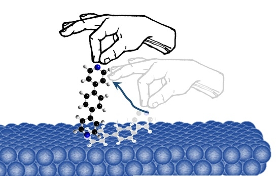
1. Introduction
Single-Shot Measurements
2. Molecular Dynamics
Challenges in Making Real-Time MD Simulations
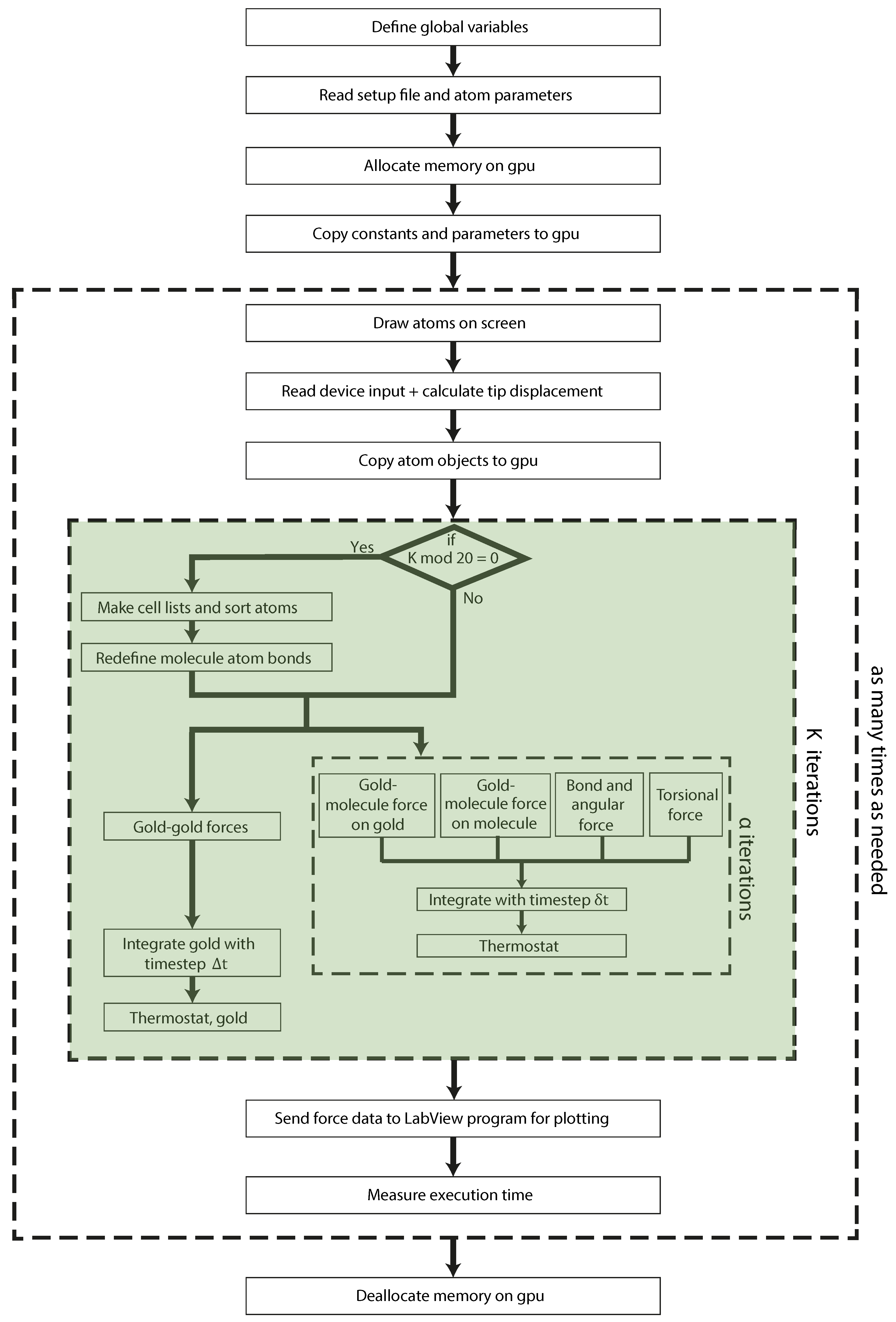
3. Molecular Dynamics: GPU Implementation
3.1. Gold-Gold Forces
3.2. Forces on Molecule Atoms
3.2.1. Gold-Molecule Forces
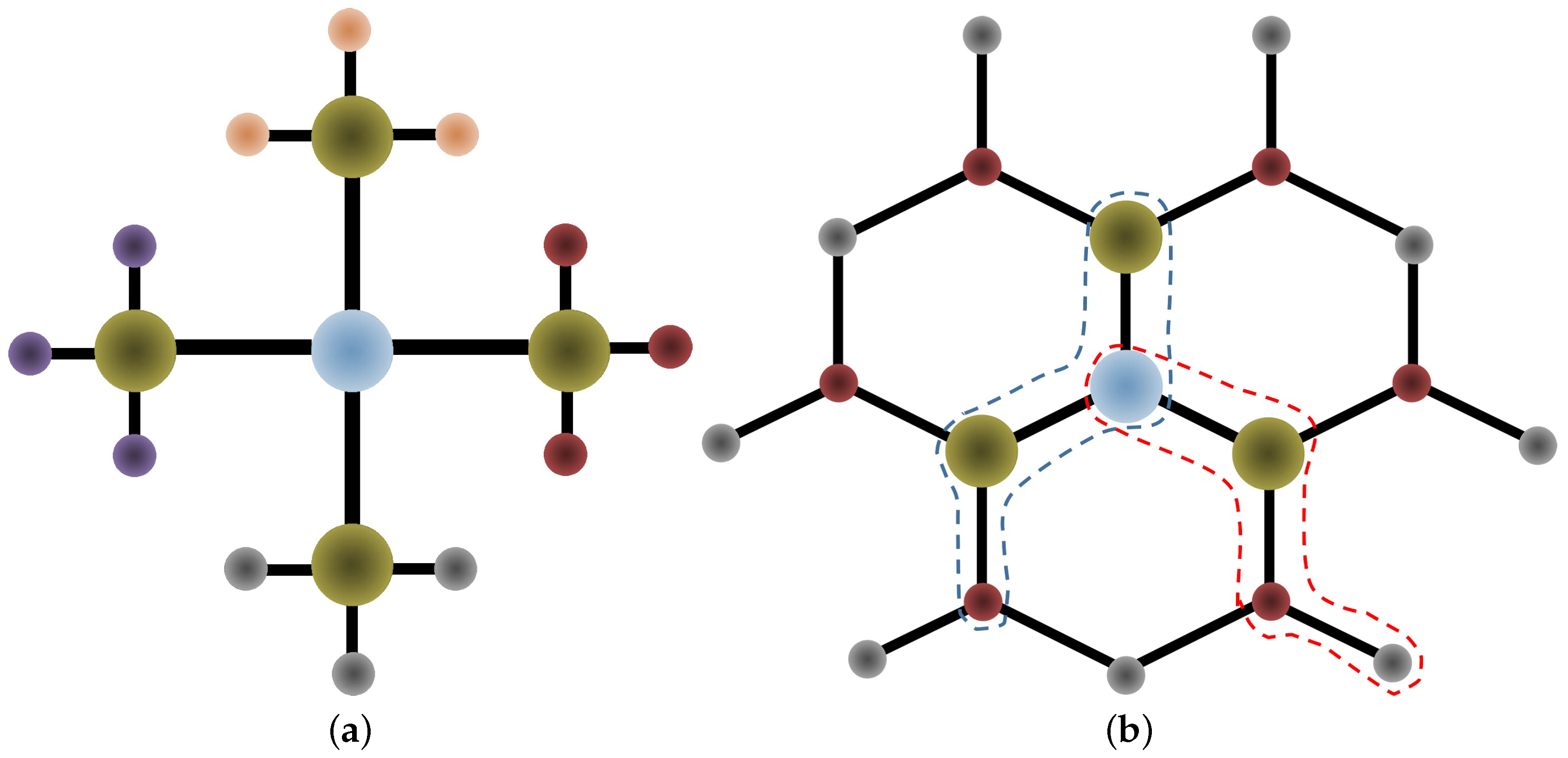
3.2.2. Intramolecular Forces
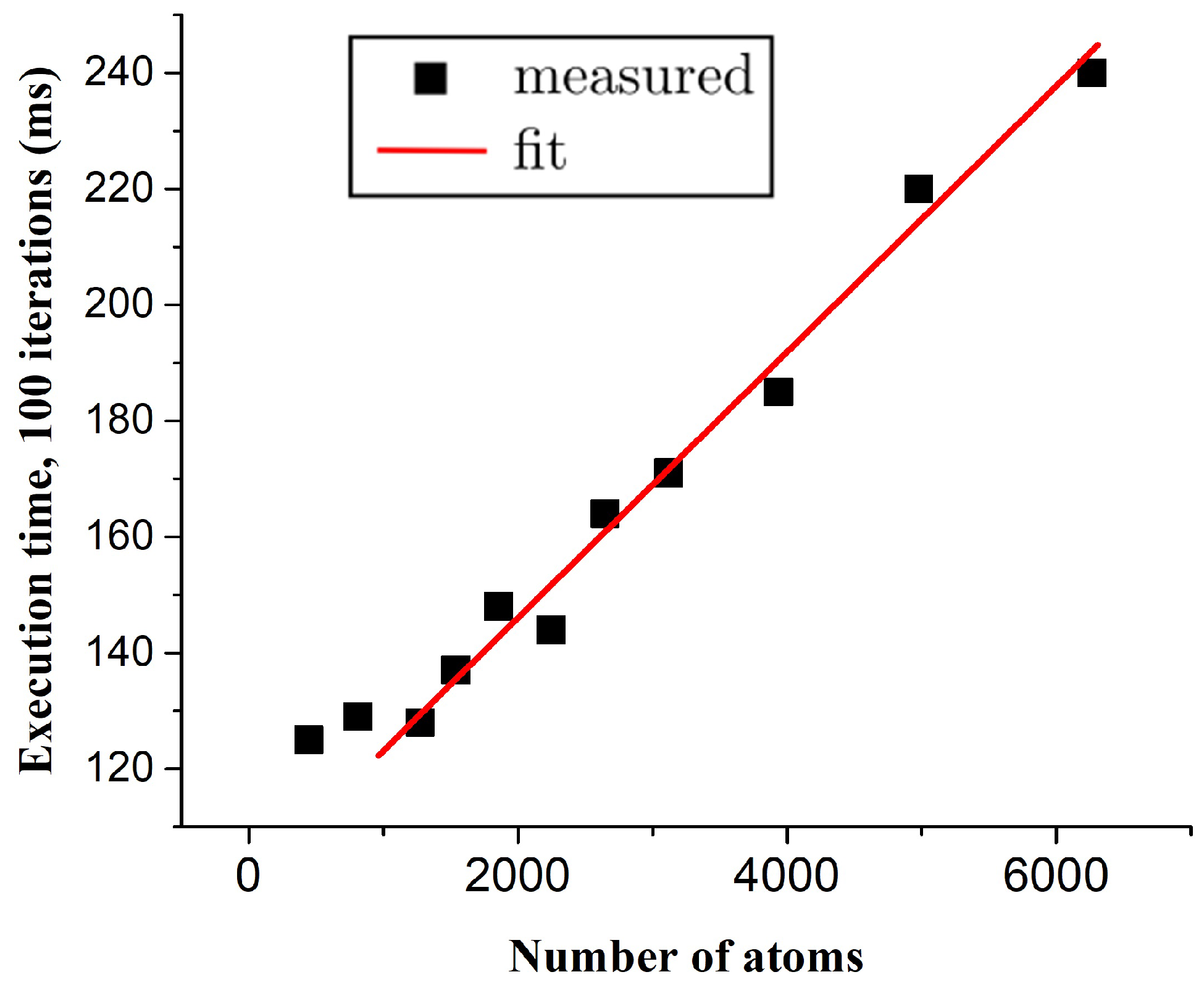
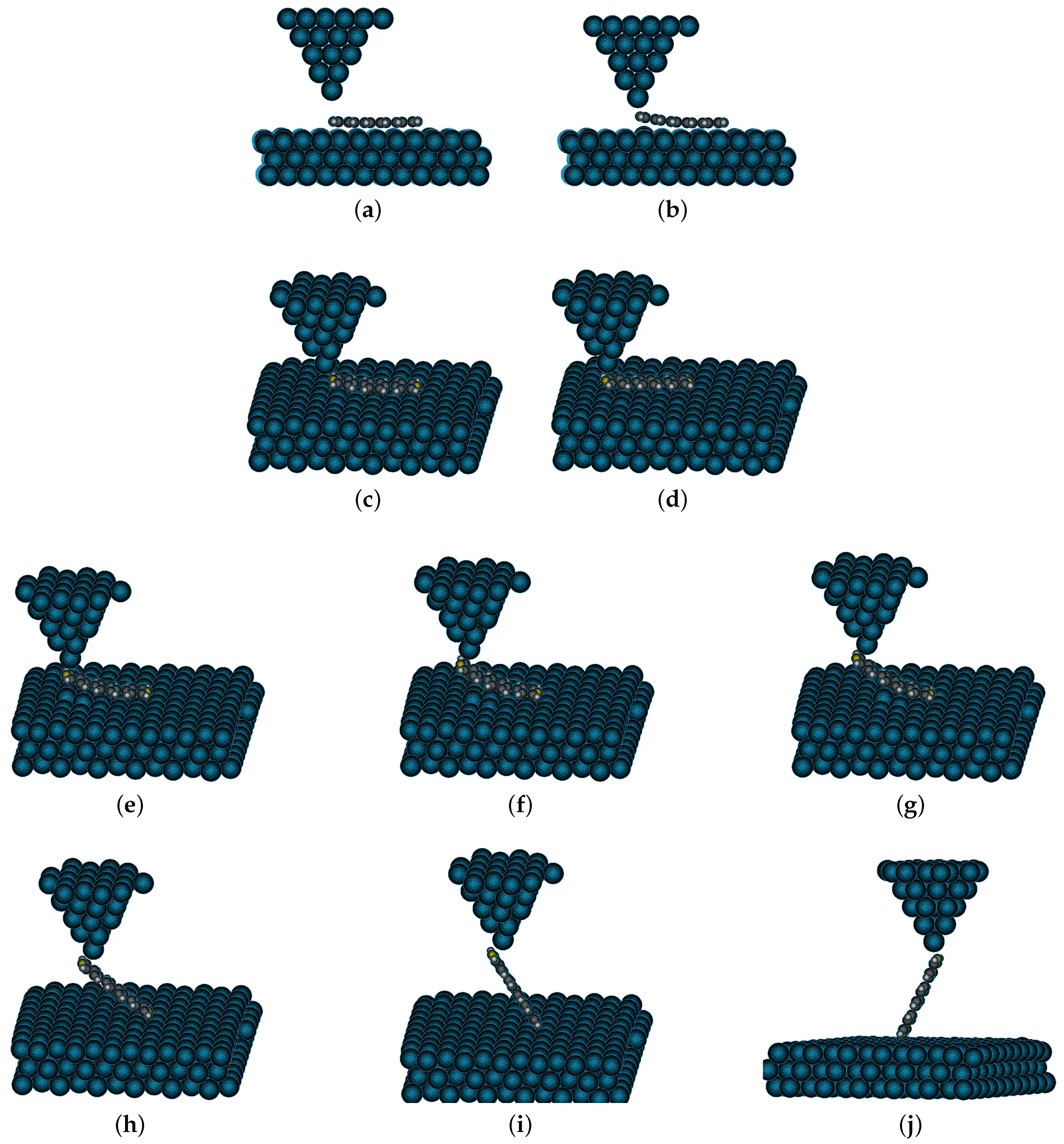
4. Results and Discussion
5. Conclusions and Outlook
Author Contributions
Funding
Acknowledgments
Conflicts of Interest
Abbreviations
| GPU | Graphics processing unit |
| GPGPU | General purpose graphics programming unit |
| CUDA | Compute unified device architecture |
| API | Application programming interface |
| CPU | Central processing unit |
| GPC | Graphics processing cluster |
| STM | Scanning tunneling microscope |
| UHV | Ultra-high vacuum |
| MD | Molecular dynamics |
| NTS | Native time-scale |
| FLOPS | Floating point operations per second |
| DFT | Density functional theory |
| NEGF | Non-equilibrium Greens function |
Appendix A. Intramolecular Forces

Appendix B. Gold-Molecule Force Calculations
Appendix B.1. Morse Potential: Au-N Bond
Appendix B.2. Lennard–Jones Potential

References
- Gimzewski, J.K.; Joachim, C. Nanoscale science of single molecules using local probes. Science 1999, 283, 1683–1688. [Google Scholar] [CrossRef] [PubMed]
- Guedon, C.M.; Valkenier, H.; Markussen, T.; Thygesen, K.S.; Hummelen, J.C.; Van Der Molen, S.J. Observation of quantum interference in molecular charge transport. Nat. Nanotechnol. 2012, 7, 305–309. [Google Scholar] [CrossRef] [PubMed]
- Ballmann, S.; Härtle, R.; Coto, P.B.; Elbing, M.; Mayor, M.; Bryce, M.R.; Thoss, M.; Weber, H.B. Experimental Evidence for Quantum Interference and Vibrationally Induced Decoherence in Single-Molecule Junctions. Phys. Rev. Lett. 2012, 109, 056801. [Google Scholar] [CrossRef] [PubMed]
- Reddy, P.; Jang, S.Y.; Segalman, R.A.; Majumdar, A. Thermoelectricity in molecular junctions. Science 2007, 315, 1568–1571. [Google Scholar] [CrossRef] [PubMed]
- Aradhya, S.V.; Venkataraman, L. Single-molecule junctions beyond electronic transport. Nat. Nanotechnol. 2013, 8, 399–410. [Google Scholar] [CrossRef] [PubMed]
- Bogani, L.; Wernsdorfer, W. Molecular spintronics using single-molecule magnets. Nat. Mater. 2008, 7, 179. [Google Scholar] [CrossRef] [PubMed]
- Burzurí, E.; van der Zant, H.S.J. Single-Molecule Spintronics. In Molecular Magnets: Physics and Applications; Springer: Berlin/Heidelberg, Germany, 2014; pp. 297–318. [Google Scholar]
- Yelin, T.; Vardimon, R.; Kuritz, N.; Korytár, R.; Bagrets, A.; Evers, F.; Kronik, L.; Tal, O. Atomically wired molecular junctions: Connecting a single organic molecule by chains of metal atoms. Nano Lett. 2013, 13, 1956–1961. [Google Scholar] [CrossRef] [PubMed]
- Kiguchi, M.; Tal, O.; Wohlthat, S.; Pauly, F.; Krieger, M.; Djukic, D.; Cuevas, J.C.; van Ruitenbeek, J.M. Highly Conductive Molecular Junctions Based on Direct Binding of Benzene to Platinum Electrodes. Phys. Rev. Lett. 2008, 101, 046801. [Google Scholar] [CrossRef] [PubMed]
- Bopp, J.M.; Tewari, S.; Sabater, C.; van Ruitenbeek, J.M. Inhomogeneous broadening of the conductance histograms for molecular junctions. Low Temp. Phys. 2017, 43, 905–909. [Google Scholar] [CrossRef]
- Kergueris, C.; Bourgoin, J.P.; Palacin, S.; Esteve, D.; Urbina, C.; Magoga, M.; Joachim, C. Electron transport through a metal-molecule-metal junction. Phys. Rev. B 1999, 59, 12505–12513. [Google Scholar] [CrossRef]
- Reichert, J.; Ochs, R.; Beckmann, D.; Weber, H.B.; Mayor, M.; Löhneysen, H.v. Driving Current through Single Organic Molecules. Phys. Rev. Lett. 2002, 88, 176804. [Google Scholar] [CrossRef] [PubMed]
- Martin, C.A.; Ding, D.; van der Zant, H.S.J.; van Ruitenbeek, J.M. Lithographic mechanical break junctions for single-molecule measurements in vacuum: Possibilities and limitations. N. J. Phys. 2008, 10, 065008. [Google Scholar] [CrossRef]
- Xu, B.; Tao, N.J. Measurement of Single-Molecule Resistance by Repeated Formation of Molecular Junctions. Science 2003, 301, 1221–1223. [Google Scholar] [CrossRef] [PubMed]
- Park, H.; Lim, A.K.L.; Alivisatos, A.P.; Park, J.; McEuen, P.L. Fabrication of metallic electrodes with nanometer separation by electromigration. Appl. Phys. Lett. 1999, 75, 301–303. [Google Scholar] [CrossRef]
- Van der Zant, H.S.J.; Kervennic, Y.V.; Poot, M.; O’Neill, K.; de Groot, Z.; Thijssen, J.M.; Heersche, H.B.; Stuhr-Hansen, N.; Bjornholm, T.; Vanmaekelbergh, D.; et al. Molecular three-terminal devices: Fabrication and measurements. Faraday Discuss. 2006, 131, 347–356. [Google Scholar] [CrossRef] [PubMed]
- Barreiro, A.; van der Zant, H.S.J.; Vandersypen, L.M.K. Quantum Dots at Room Temperature Carved out from Few-Layer Graphene. Nano Lett. 2012, 12, 6096–6100. [Google Scholar] [CrossRef] [PubMed]
- Lau, C.S.; Mol, J.A.; Warner, J.H.; Briggs, G.A.D. Nanoscale control of graphene electrodes. Phys. Chem. Chem. Phys. 2014, 16, 20398–20401. [Google Scholar] [CrossRef] [PubMed]
- Joachim, C.; Gimzewski, J.K.; Schlittler, R.R.; Chavy, C. Electronic Transparence of a Single C60 Molecule. Phys. Rev. Lett. 1995, 74, 2102–2105. [Google Scholar] [CrossRef] [PubMed]
- Haiss, W.; Nichols, R.J.; van Zalinge, H.; Higgins, S.J.; Bethell, D.; Schiffrin, D.J. Measurement of single molecule conductivity using the spontaneous formation of molecular wires. Phys. Chem. Chem. Phys. 2004, 6, 4330–4337. [Google Scholar] [CrossRef]
- Haiss, W.; Wang, C.; Grace, I.; Batsanov, A.S.; Schiffrin, D.J.; Higgins, S.J.; Bryce, M.R.; Lambert, C.J.; Nichols, R.J. Precision control of single-molecule electrical junctions. Nat. Mater. 2006, 6, 995–1002. [Google Scholar] [CrossRef] [PubMed]
- Temirov, R.; Lassise, A.; Anders, F.B.; Tautz, F.S. Kondo effect by controlled cleavage of a single-molecule contact. Nanotechnology 2008, 19, 065401. [Google Scholar] [CrossRef] [PubMed]
- Jasper-Tönnies, T.; Garcia-Lekue, A.; Frederiksen, T.; Ulrich, S.; Herges, R.; Berndt, R. Conductance of a Freestanding Conjugated Molecular Wire. Phys. Rev. Lett. 2017, 119, 066801. [Google Scholar] [CrossRef] [PubMed]
- Tewari, S. Molecular Electronics: Controlled Manipulation, Noise and Graphene Architecture. Ph.D. Thesis, Leiden Institute of Physics (LION), Leiden University, Leiden, The Netherlands, 2018. [Google Scholar]
- Tewari, S.; Bakermans, J.; Wagner, C.; Galli, F.; van Ruitenbeek, J.M. Intuitive human interface to a scanning tunneling microscope: Observation of parity oscillations for a single atomic chain. Phys. Rev. X 2018. submitted. [Google Scholar]
- Green, M.F.B.; Esat, T.; Wagner, C.; Leinen, P.; Grötsch, A.; Tautz, F.S.; Temirov, R. Patterning a hydrogen-bonded molecular monolayer with a hand-controlled scanning probe microscope. Beilstein J. Nanotechnol. 2014, 5, 1926. [Google Scholar] [CrossRef] [PubMed] [Green Version]
- Leach, A.R. Molecular Modelling: Principles and Applications; Pearson Education: Upper Saddle River, NJ, USA, 2001. [Google Scholar]
- Tuckerman, M.E.; Berne, B.J.; Rossi, A. Molecular dynamics algorithm for multiple time scales: Systems with disparate masses. J. Chem. Phys. 1991, 94, 1465–1469. [Google Scholar] [CrossRef]
- Kuroda, Y.; Suenaga, A.; Sato, Y.; Kosuda, S.; Taiji, M. All-atom molecular dynamics analysis of multi-peptide systems reproduces peptide solubility in line with experimental observations. Sci. Rep. 2016, 6, 19479. [Google Scholar] [CrossRef] [PubMed]
- Van Meel, J.A.; Arnold, A.; Frenkel, D.; Portegies Zwart, S.; Belleman, R.G. Harvesting graphics power for MD simulations. Mol. Simul. 2008, 34, 259–266. [Google Scholar] [CrossRef]
- Anderson, J.A.; Lorenz, C.D.; Travesset, A. General purpose molecular dynamics simulations fully implemented on graphics processing units. J. Comput. Phys. 2008, 227, 5342–5359. [Google Scholar] [CrossRef]
- Zhang, X.; Guo, W.; Qin, X.; Zhao, X. A Highly Extensible Framework for Molecule Dynamic Simulation on GPUs. In Proceedings of the International Conference on Parallel and Distributed Processing Techniques and Applications (PDPTA), Las Vegas, NV, USA, 22–25 July 2013; p. 524. [Google Scholar]
- Yao, Z.; Wang, J.S.; Liu, G.R.; Cheng, M. Improved neighbor list algorithm in molecular simulations using cell decomposition and data sorting method. Comput. Phys. Commun. 2004, 161, 27–35. [Google Scholar] [CrossRef]
- Chialvo, A.A.; Debenedetti, P.G. On the use of the Verlet neighbor list in molecular dynamics. Comput. Phys. Commun. 1990, 60, 215–224. [Google Scholar] [CrossRef]
- Harris, M. Optimizing Parallel Reduction in CUDA; NVDIA Developer Technology: Santa Clara, CA, USA, 2008; Available online: http://developer.download.nvidia.com/compute/DevZone/C/html/C/src/reduction/doc/reduction.pdf (accessed on 28 May 2018).
- Alsop, J.; Sinclair, M.D.; Komuravelli, R.; Adve, S.V. GSI: A GPU stall inspector to characterize the sources of memory stalls for tightly coupled GPUs. In Proceedings of the 2016 IEEE International Symposium on Performance Analysis of Systems and Software (ISPASS), Uppsala, Sweden, 17–19 April 2016; pp. 172–182. [Google Scholar]
- Kraft, A.; Temirov, R.; Henze, S.K.M.; Soubatch, S.; Rohlfing, M.; Tautz, F.S. Lateral adsorption geometry and site-specific electronic structure of a large organic chemisorbate on a metal surface. Phys. Rev. B 2006, 74, 041402. [Google Scholar] [CrossRef]
- Rascón-Ramos, H.; Artés, J.M.; Li, Y.; Hihath, J. Binding configurations and intramolecular strain in single-molecule devices. Nat. Mater. 2015, 14, 517–522. [Google Scholar] [CrossRef] [PubMed]
- Fournier, N.; Wagner, C.; Weiss, C.; Temirov, R.; Tautz, F.S. Force-controlled lifting of molecular wires. Phys. Rev. B 2011, 84, 035435. [Google Scholar] [CrossRef] [Green Version]


| CUDA Device Name | GeForce GTX 960 |
|---|---|
| Compute capability | 5.2 |
| Floating-point performance | 2.413 TFLOPS |
| GPC count | 2 |
| SMMper GPC | 4 |
| Cores per SMM | 128 |
| Threads per SMM | 2048 |
| Max # of threads per block | 1024 |
| Max block size | 1024 × 1024 × 64 |
| Max grid size | 2,147,483,647 × 65,535 × 65,535 |
| Warp size | 32 threads |
| Max # active warps per SMM | 64 warps |
© 2018 by the authors. Licensee MDPI, Basel, Switzerland. This article is an open access article distributed under the terms and conditions of the Creative Commons Attribution (CC BY) license (http://creativecommons.org/licenses/by/4.0/).
Share and Cite
Van Vreumingen, D.; Tewari, S.; Verbeek, F.; Van Ruitenbeek, J.M. Towards Controlled Single-Molecule Manipulation Using “Real-Time” Molecular Dynamics Simulation: A GPU Implementation. Micromachines 2018, 9, 270. https://doi.org/10.3390/mi9060270
Van Vreumingen D, Tewari S, Verbeek F, Van Ruitenbeek JM. Towards Controlled Single-Molecule Manipulation Using “Real-Time” Molecular Dynamics Simulation: A GPU Implementation. Micromachines. 2018; 9(6):270. https://doi.org/10.3390/mi9060270
Chicago/Turabian StyleVan Vreumingen, Dyon, Sumit Tewari, Fons Verbeek, and Jan M. Van Ruitenbeek. 2018. "Towards Controlled Single-Molecule Manipulation Using “Real-Time” Molecular Dynamics Simulation: A GPU Implementation" Micromachines 9, no. 6: 270. https://doi.org/10.3390/mi9060270