A Review of Trends for Corrosion Loss and Pit Depth in Longer-Term Exposures


Centre for Infrastructure Performance and Reliability, The University of Newcastle, Newcastle, NSW 2308, Australia
Corros. Mater. Degrad. 2020, 1(1), 42-58; https://doi.org/10.3390/cmd1010004
Submission received: 19 June 2018
/
Revised: 2 July 2018
/
Accepted: 17 July 2018
/
Published: 18 July 2018
Abstract
:For infrastructure applications in marine environments, the eventual initiation of corrosion (and pitting) of steels (and other metals and alloys) often is assumed an inescapable fact, and practical interest then centres on the rate at which corrosion damage is likely to occur in the future. This demands models with a reasonable degree of accuracy, preferably anchored in corrosion theory and calibrated to actual observations under realistic exposure conditions. Recent developments in the understanding of the development of corrosion loss and of maximum pit depth in particular are reviewed in light of modern techniques that permit much closer examination of pitted and corroded surfaces. From these observations, and from sometimes forgotten or ignored observations in the literature, it is proposed that pitting (and crevice corrosion) plays an important role in the overall corrosion process, but that longer term pitting behaviour is considerably more complex than usually considered. In turn, this explains much of the, often high, variability in maximum depths of pits observed at any point in time. The practical implications are outlined.
1. Introduction
Despite their proneness to corrosion, particularly if not well-protected, mild and low alloy structural steels remain important economic construction materials in marine offshore and marine coastal industrial environments. In part, this is because of their relative ease of use in construction in hostile environments, their high strength to weight ratio and also their relatively lower down-time costs for maintenance. Particularly in the offshore environment, for shipping, naval defence facilities and structures in coastal industrial environments, corrosion is an important aspect of overall facility management [1,2,3] and estimates of the likely rate or development of future corrosion of considerable practical interest [4]. For these applications, it is recognized that corrosion tests under laboratory conditions, such as short-term exposures in artificial seawaters, electrochemical tests or accelerated tests are of limited value, mainly because the results from such tests are difficult to relate to longer term corrosion behaviour. Because of these practical demands, renewed efforts have been made in the last two decades to develop more realistic models for corrosion. For estimating the likely structural strength and structural reliability of structures, models for predicting the development of general corrosion loss are critical [5]. Pitting is of interest more for liquid retaining or exclusion systems such as pipelines, tanks and cofferdams or sheet piling, but for these, too, prediction of pit depth development is of much interest [3].
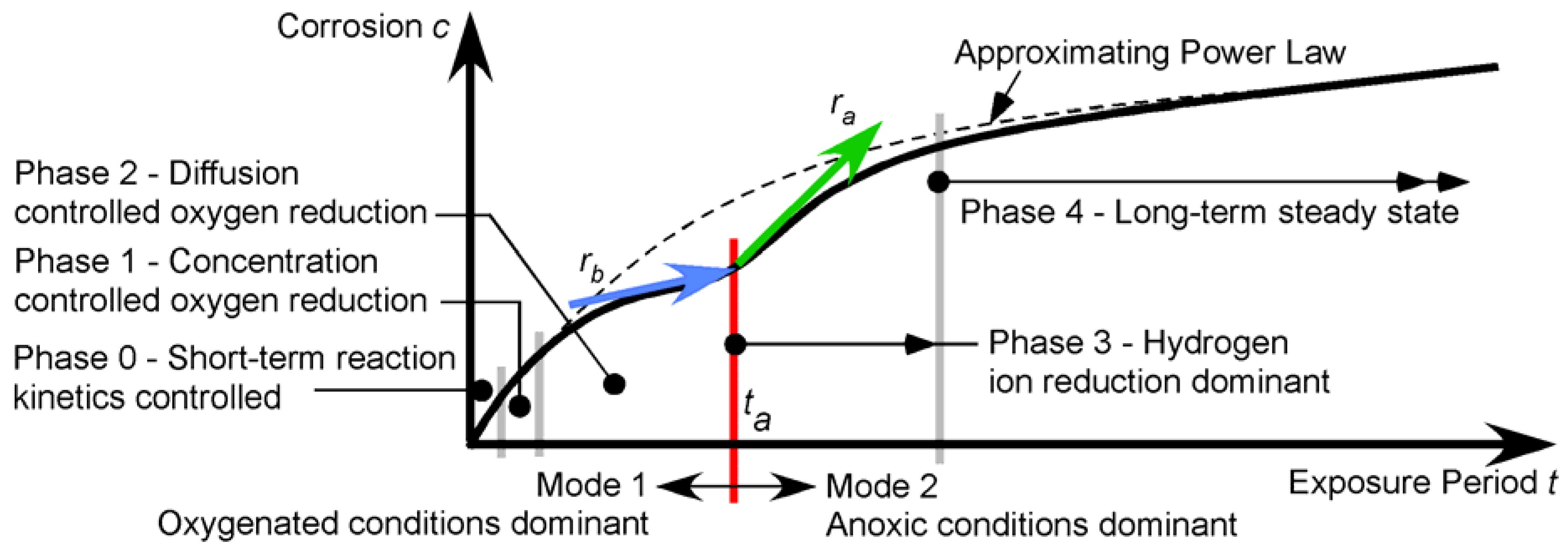
Careful examination of data and consideration of the corrosion mechanisms that may be involved have shown that for the general or ‘uniform’ corrosion, or corrosion as measured by mass loss as a function of exposure time, the bi-modal characteristic (Figure 1) is more appropriate than earlier models [6]. This model has been shown to be suitable for the longer term exposure of steels, cast irons and aluminium and copper alloys to a wide variety of natural exposure environments, including immersion (fresh and marine), tidal and various atmospheric exposure zones [7,8,9], as well as for ferrous metals in soils [10].
While the actual mass loss values and the timing of the phases shown in Figure 1 depend very much on the metal or alloy and on the environment, the overall characteristic is pervasive. It is at odds with the conventional power law function that has its roots in the original derivation by Tammann in 1923 [11] and refined and examined by many authors [12,13,14]. The power law has mathematical deficiencies in meeting the conditions for the corrosion process at t = 0, as well as other issues [14], although it could be taken as an approximation to the bi-modal model for the early period of exposure, that is from Time 0–ta (Figure 1), during which time, the corrosion process is assumed to be predominantly under oxygen diffusion control. This is shown as Mode 1. Subsequently, in Mode 2, the corrosion processes according to the bi-modal model are predominantly under anoxic conditions. In each of these two modes, the model has a number of different phases, each of which idealize the dominant corrosion process at that time. The details have been given many times (e.g., [7]) and need not be rehearsed here.
The critical issue for an explanation of the bi-modal behaviour is the change at ta from a very low instantaneous corrosion rate rb before ta is reached to ra almost immediately after it, although in practice, there is some short transition period (Figure 1). Given that the bi-modal characteristic is seen for a range of aluminium alloys and for many copper alloys (but not for ‘pure’ copper in ‘pure’ water [15]), as well as for many different steels including high chromium steels, it follows that it is not primarily a function of the type of material. Moreover, it has been shown that small changes in steel composition (including carbon content) have little effect on the mass losses or on the bi-modal characteristic [16,17]. Similarly, the bi-modal characteristic is seen for the outer skin of cast irons, as well as for machined cast irons in the same environment [18]. In this context, it is interesting that for steels (and cast irons) buried in soils, the degree of compaction, and by implication the air-void content next to the metal surface, has a major influence on the amount of corrosion, but not on the general form (topology) of the bi-modal characteristic [10].
Using the limited data that were available at the time, it was proposed that the bi-modal characteristic also applies to longer term trends for maximum and average pit depths [19]. Some relationship between them might be expected particularly for metals that corrode mainly by pitting since mass loss caused by pitting is included automatically and predominantly in the overall mass loss. In other cases, such as for steels, pit depth usually is corrected by increasing it by the corrosion loss equivalent to the mass loss, on the basis that the mass loss in pitting is very small compared to overall mass loss [20]. However, more detailed observations, including extensive microscope observations of the surfaces of steel samples recovered from marine corrosion immersion environments, have suggested a more complex relationship between the bi-modal trend for corrosion loss and the pitting of the steel surfaces. This is explored in the present paper. Largely, it reinterprets data already in the literature to present a new view of the interaction between pitting corrosion and trends for mass loss or uniform corrosion.
The next section reviews a selection of data for pitting to consider the relation between pitting corrosion and mass loss initially in an oxygen-rich environment, followed by such corrosion in the oxygen-poor environment created by the development of heavy rusts, including the presence of magnetite and possibly hematite. Based on detailed and extensive experimental observations for steels subject to extended exposures in a marine immersion environment, the following section provides a hypothesis for the processes involved in the progression of pitting through Mode 1 to the start of Mode 2 of the bi-modal model. It includes photographs of corroded surfaces after superficial rusts have been removed, carefully, so as not to destroy the patterns and features of the underlying metal as created by the interaction of the corroding steel surface and the overlying rusts. Some comments are then made about what could be expected to be observed in new experimental programs with careful observation. Practical implications are discussed briefly.
2. Trends in Pit Depth and Corrosion Loss
It is sometime claimed that mild and structural steels do not ‘pit’, but rather that they suffer from ‘localized corrosion’, based on the notion that only a run-out of corrosion current i on an E-i plot as obtained in an electrochemical experiment denotes pitting. A little reflection will show that this type of electrochemical behaviour is observable only for metals with passive films, such as stainless steels and aluminium alloys, and is considered the direct result of breaching of the passive film, without which it is claimed pitting cannot occur [21]. On the other hand, the term pitting has been applied also to mild steels exposed to alkaline solutions, such as seawater, and has been so for many decades [13,22,23,24], despite the passive film on mild and low alloys steels being accepted as weak and unable to have any significant passivity effect [21]. This is consistent also with the Pourbaix [25] diagram for mild steel in chloride-rich waters. Herein, we follow the classic convention and apply the term pitting also for mild and low alloy steels in seawater.
The detailed work of Butler et al. [23] showed that for (almost) pure iron and some other ferrous metals in alkaline solutions, pitting commenced very quickly (within days), showing circular or near-circular pits, usually exhibiting shiny bases, that extended only some way into the metal, that is the pits appeared to be limited in depth. Butler et al. [23] noted that usually, each pit was associated with a ring of corrosion product around and over the pit mouth and that this region was slightly alkaline. These observations are consistent with pitting theories such as that advanced by Wranglen [26]. Butler et al. [23] also observed that, after removal of the rusts, new or ‘daughter’ pits had formed at the peripheries of the corrosion product mounds, giving rise to small clusters of pits. This is in contrast to observations that pitting of stainless steels appears to show ‘minimum distances’ between pits, at least for shorter exposure periods [27].
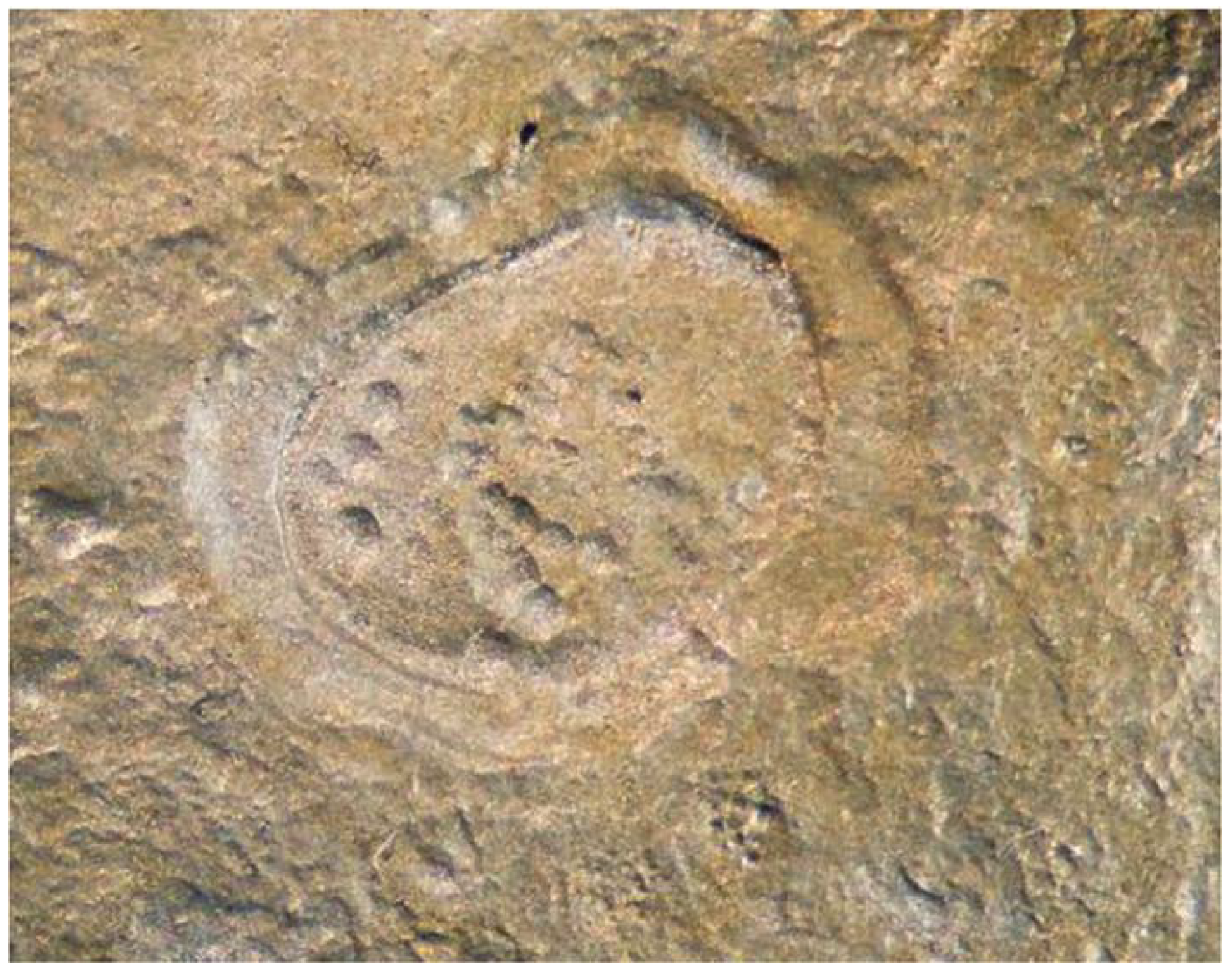
For mild steels immersed for long periods (years) in seawater, pit depth development has been observed [28] to occur in what appear to be steps in pit depth, with early pitting producing plateaus, these plateaus then permitting new pitting. That new pitting then, in turn, produced new, lower corrosion plateaus that, in turn, allowed further, deeper pitting. Figure 2 shows that pattern. It suggests immediately that the pitting corrosion process, for mild steels at least, is more complex than simple smooth, gradual, growth in pit depth with increased exposure time, as is the behaviour usually proposed or assumed in standard texts. Importantly, the pattern shown in Figure 2 was observed only when the exposure period was sufficiently long in time, and there were observations sufficiently close in time to note the changing corrosion patterns. In this context, it has been shown recently that the pitting of cast iron surfaces buried in soils shows distinct cohorts of pit depths, all roughly of similar pit depth increments [29]. It is thus of interest whether a similar pattern can be seen for immersion corrosion in data that so far have not been considered.
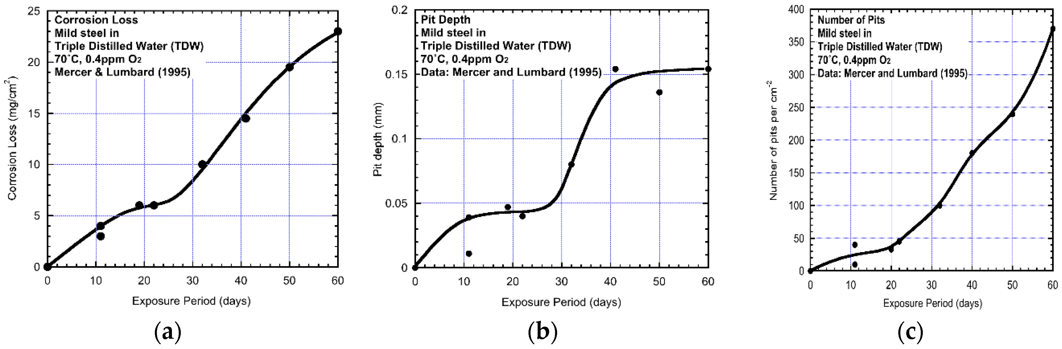
Evidence for the stepped pattern of pit depth development can be discerned also in some literature data for the corrosion and pitting of steels. Thus, in well-controlled and well-monitored tests, Mercer and Lumbard [24] noted that pitting became limited in depth very soon after first exposure. This limited development of pit depth was observed for mild steels in a variety of exposure environments, including triply-distilled water (TDW), Teddington (hard) drinking-water, brackish water and transported seawater. They measured both mass loss and pit depth and also counted the number of pits per unit area. Figure 3 shows data for mild steel in TDW at 70 °C and under quite low oxygen concentration conditions. It is acknowledged that in these data and the others to follow, there is a degree of uncertainty or variability in the reported pit depth or mass loss. In many cases, there is insufficient data to ascertain data variability; however, some estimates have been made in specially conducted experiments, and such variability (or scatter) in the data was shown to be small [30,31].
The data trends in Figure 3 have been added and were not provided by Mercer and Lumbard [24]. These authors made little comment about the data and any trending, including the possibility that the data for mass loss at least (Figure 3a) can be readily interpreted as having an obvious bi-modal character
Figure 3b for pit depth also appears to show bi-modal trending. It also shows that pit depth reached a peak value soon after first exposure and that maximum pit depth increased relatively little for some time thereafter. Comparing with Figure 3a shows that mass-loss increased roughly in concert with the number of pits per unit area. Interestingly, the upswing in the trend for pit depth and that for mass-loss occur at a very similar time: 25–30 days after first exposure, shown as time ta on all three plots. Figure 3c shows the number of pits as a function of time and that this number increases in the period immediately after ta, i.e., during the period 30–40 days. It is possible also to read into Figure 3c that there is a higher rate of pit formation in the very early period, i.e., in the period 0–10 days. This is consistent with the observations by Butler et al. [23].
Further, Figure 3 shows the relationships between a major increase in pit depth, the number of pits and corrosion loss as measured by mass loss. In particular, the duration of Mode 1 (cf. Figure 1) as measured by ta is essentially the same for pit depth and for mass loss, being, for these exposure conditions, around 27 days. The consistency between the change-over time ta from Mode 1 to Mode 2 was noted also for a number of other datasets, although for much longer times ta [32].
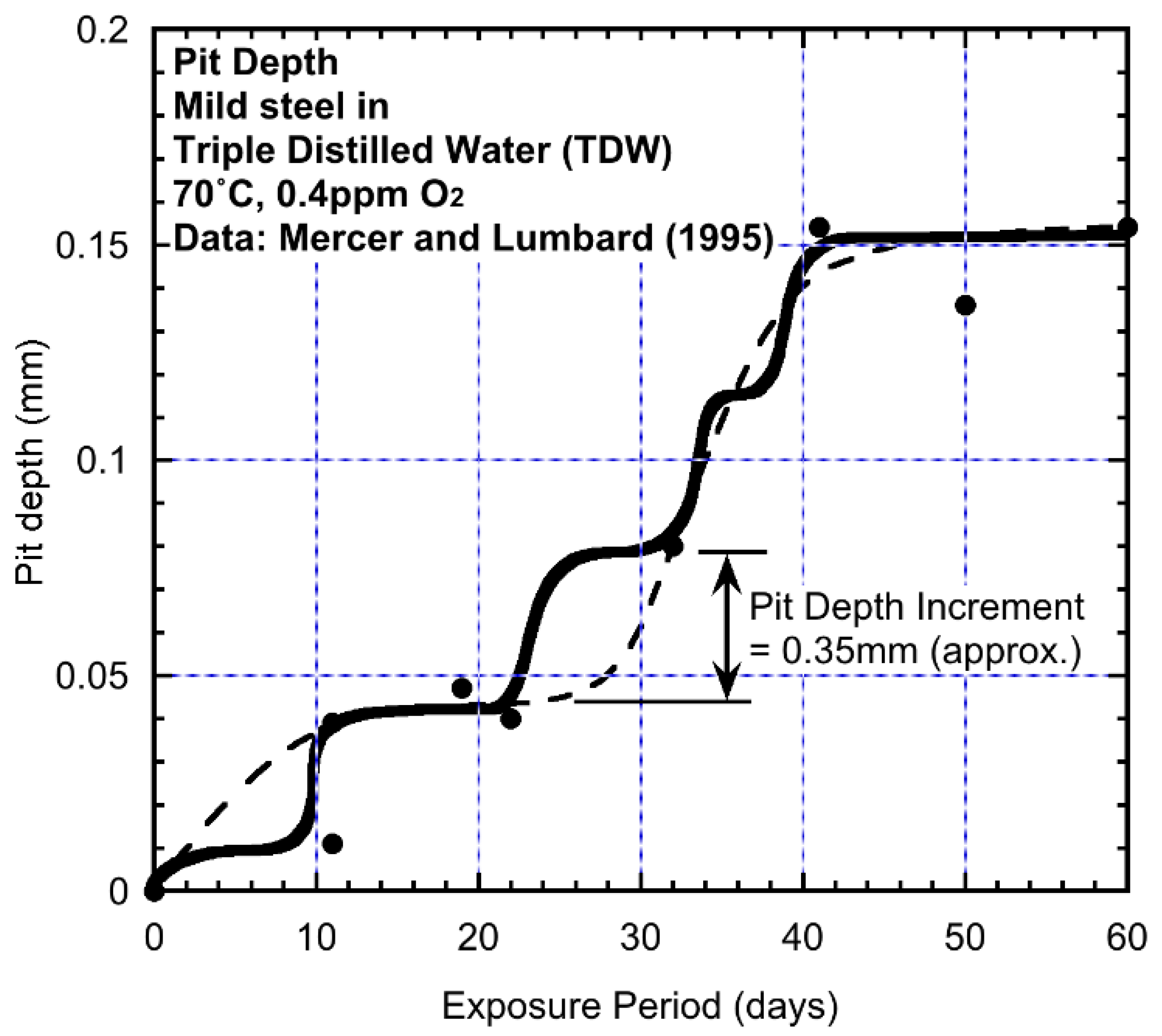
The data for pit depth (Figure 3b) can be re-interpreted using the notion that pit depth development occurs in stages, as is implicit in Figure 2. Although the amount of data for pit depths is limited, a possible re-interpretation of the data in Figure 3b is given in Figure 4, using also the notion that pit depth increments are likely to be of similar value.
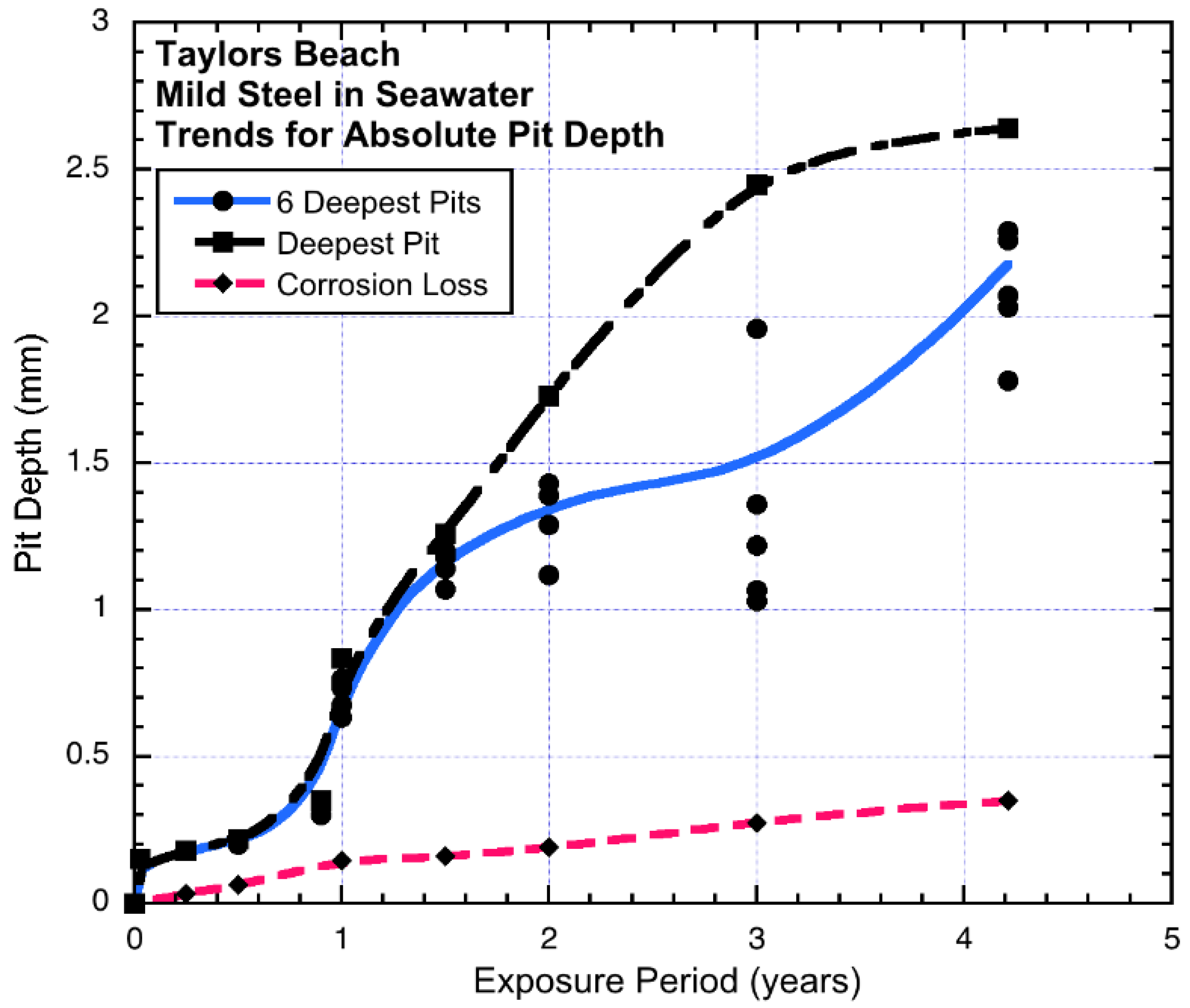
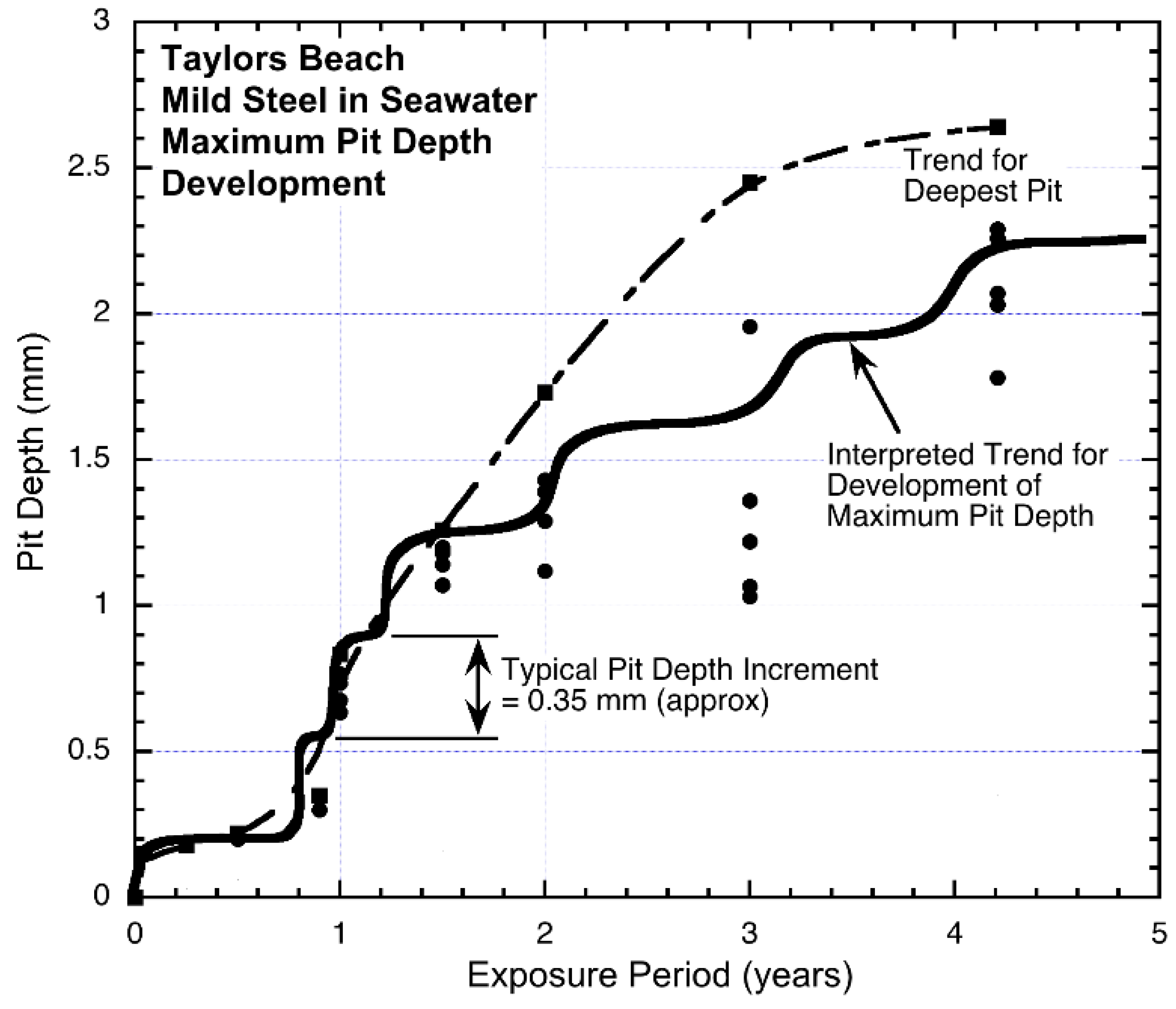
Generally, similar observations have been made for field exposure of mild steels in seawater immersion over periods of up to 3–4 years, carried out at Taylors Beach. In one of the earlier programs, both mass loss (general corrosion) and pit depths were recorded and reported. Particularly for the latter, the maximum pit depth, as well as the next six deepest pits were reported [23]. Figure 5 shows the results. It is seen that the maximum pit depth and the average pit depth are reached quite early and then become almost steady at about 0.25 mm, until ta ≈ 1 year is reached, at which time both trends increase. The trend for the deepest pit increases some considerable amount, but the average trend for the six deepest pits (i.e., including the deepest pits) can be interpreted as consisting of stepped increments in pit depth of about 0.35 mm (Figure 6).
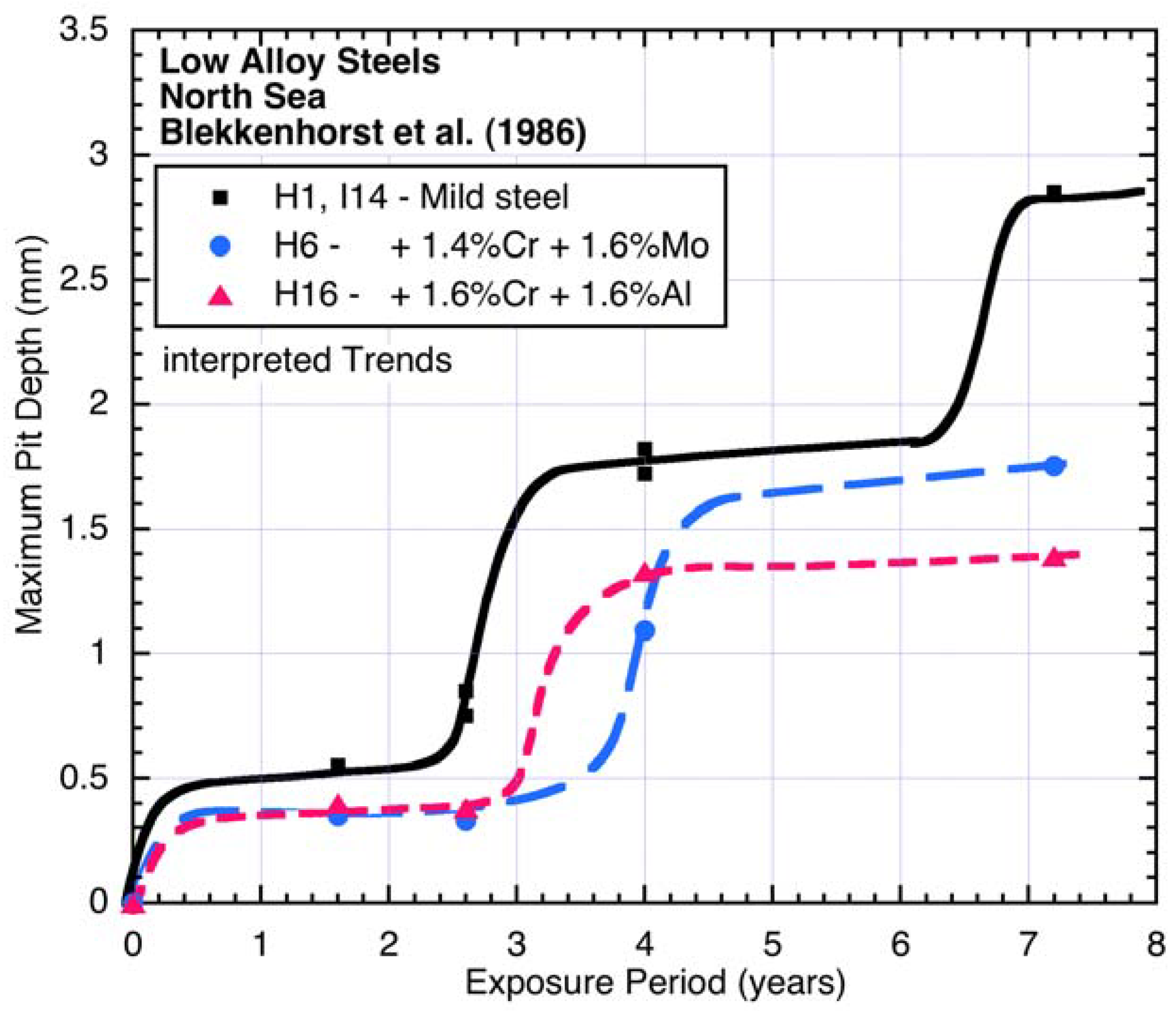
A similar comparison between the trends for maximum pit depth can be seen for a variety of steels immersion exposed in the North Sea for 7.2 years [33]. Just three examples of the matching datasets for maximum pit depth are shown in Figure 7 together with added trends. In these cases, the increment in pit depth is around 1.0 mm. Almost certainly, this can be attributed to the high level of nutrient pollution in the North Sea [34] contributing to microbiologically-influenced corrosion and causing more severe and much deeper pitting [35]. The severe pitting caused by high levels of nutrient pollution has been observed also off the coast of Nigeria in oil exploration areas [36]. The important point here is the stepped, progressive, development of pit depth. Quantification of the effect of nutrient pollution on such pit depth incrementation remains a matter for further investigation.
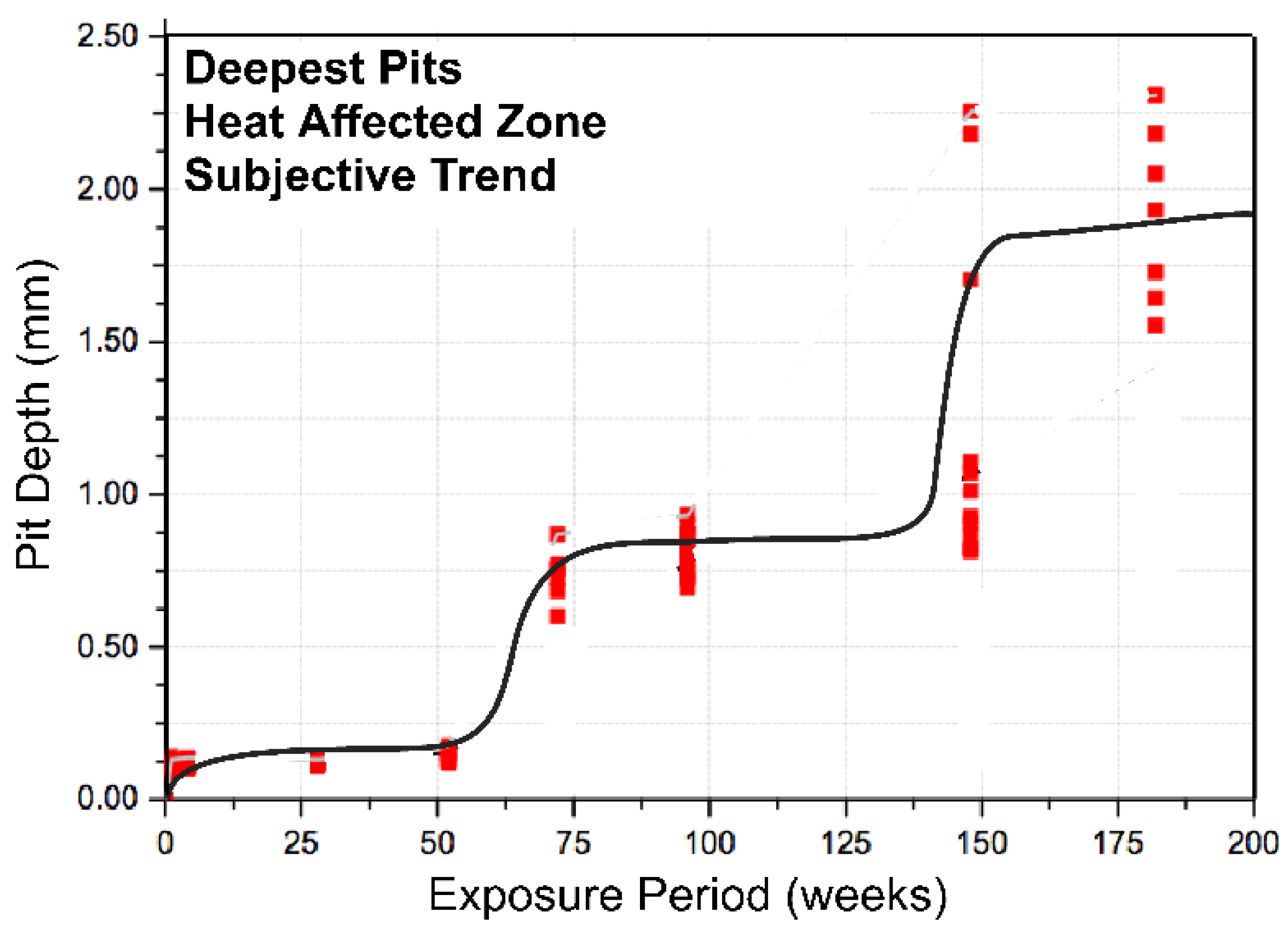
A further example can be seen in the experimental results for the 6–8 deepest pits measured in the heat-affected zone of the longitudinal fusion weld of a steel pipeline [37]. The results are shown in Figure 8, again with interpreted trends added. It shows the same kind of progressive increase in pit depth as before.
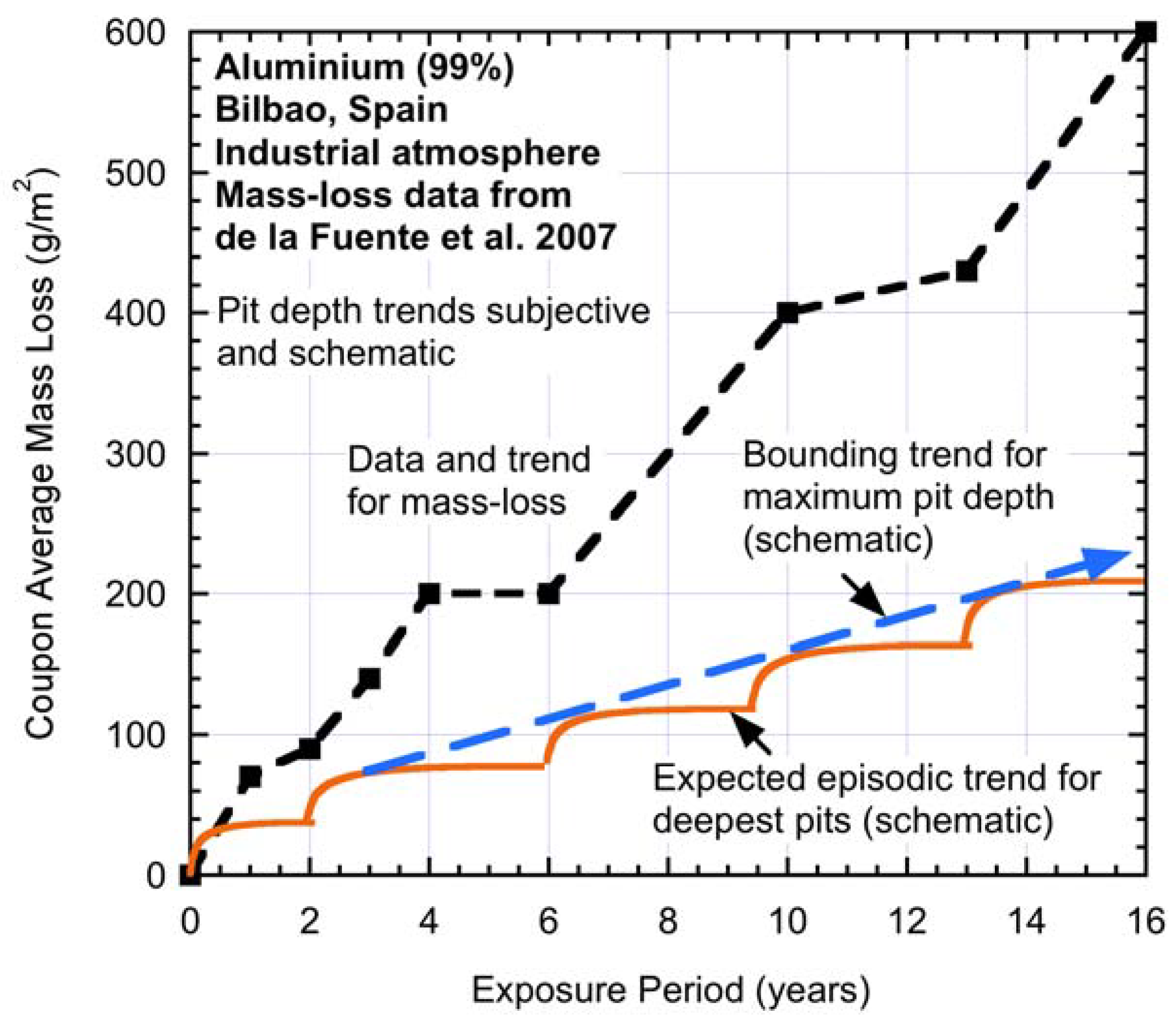
As a further example, consider Figure 9 for the mass loss of a 99% (wt) pure aluminium alloy [38]. In the case of aluminium alloys, general or uniform corrosion is almost negligible, and the predominant corrosion mechanism is by pitting [39]. It might thus be expected that average mass loss at any one time represents, in some way, the average depth of pitting, and this can be expected to be similar over a surface for a given period of exposure. This is not to say that there will not be some pits that are deeper, but the majority of pitting is likely to be similar (cf. Figure 2). Figure 9 shows the data for mass loss and the step-wise interpreted trend. Also added, entirely schematically, is what might be the expected step-wise, or episodic, development of pit depth. Clearly, this is not definitive, but suggests it as a topic for further investigation.
3. Mechanism for the Development of Pitting Corrosion
It is useful to review some basic notions for the development of pitting corrosion, particularly in seawater conditions. For the present purposes, the possible distinction between pitting on passive film metals and localized corrosion on others is not considered crucial for the discussion to follow, and the term pitting is used throughout. Most of the theories for the initiation and development of pitting focus on the way a pit can initiate on what is close to a perfect surface, with material imperfections, inclusions and local alloy constituents producing only very small differences in local potential to drive dissolution that can lead to pit initiation [22,40,41]. Initial pitting usually is considered to initiate at multiple sites on the surface of a metal. Only some become stable pits able to propagate with time. The following discussion is focussed entirely on the propagation of pits beyond the period in which pits become stable. Figure 10 gives a schematic representation of the process.
Usually, it is considered that soon after a pit enters into a stable growth mode, it is necessary for the pit mouth to have a degree of cover so as to prevent the contents of the pit from interacting with the environment and thereby rendering the pit passive [40,41,42]. For mild steels, this occurs relatively quickly, and already soon after becoming stable, the pits show localized corrosion product around and over the pit mouth [23]; this soon develops into widespread cover by corrosion products (Figure 11).
As is well established, as each pit develops in size, the interior becomes sufficiently far removed from the pit mouth to render oxygen diffusion into the pit more difficult. Furthermore, the corrosion products, particularly the magnetite layer (Figure 10c), retard diffusion processes. The net effect is that anoxic conditions can develop inside the pits. In turn, these permit conditions suitable for autocatalytic reactions to commence [26]. This occurs with dissociation of water and hydrogen ions replacing oxygen as the electron acceptor within the pit, with hydrogen gas evolving from the inside surfaces of the pit. The resulting pressure then usually causes the rupture of the covering corrosion product, allowing gas effusion through the pit mouth [40]. An example of a ruptured corrosion product over pit mouths is shown in Figure 11.
As corrosion progresses, the magnitude of the exterior corrosion product will increase, and overall diffusion into and out of the pit will become more difficult. The mechanisms involved have been considered in detail by Wranglen [26], who noted the low pH inside the pits and the likelihood of autocatalytic reactions. Although secondary expositions of his work always refer to chlorides as essential for the process, this was not part of Wranglen’s exposition. He simply required a potential to drive the process (although he did attribute much of this to manganese sulphide inclusions). More generally, the potential driving pitting can be the result of any imperfections [40]. However, it should be clear that as pit depth increases, the net potential for further pit depth development becomes, slowly, exhausted, and growth in pit depth stops. Overall, these steps are shown in Figure 10a.
It might be noted that for shorter term exposures, such as typical in laboratory observations of pitting corrosion, the notion of a limited pit depth caused much discussion in the corrosion literature, as summarized, for example, by Frankel [41]. The limited depth to which pits can propagate has been identified with the IR (I = current, R = resistance) or potential V (volts) drop through the depth of the pit and the rust layers, that is between the cathodic region around the pit mouth and the anodic base of the pit [43]. It does not depend directly on the external environment other than that a cathode can exist somewhere outside the pit. Galvele [42] considered the sharp transition between the alkaline region immediately around a pit mouth and the acidic pit interior and concluded that diffusion of species into and out of the pit was an important part in explaining experimental observations. This and similar work provided a basis for numerical simulation of the pitting process and the progression of pit depth. Using an idealized pit geometry and models of the electrochemical reactions and the diffusion processes involved, Sharland and Tasker [44], Turnbull [45] and others showed that the limited depth concept existed and could be simulated. It also could be calibrated (indirectly) to electrochemical experimental results [46]. However, physical evidence such as shown in Figure 2 was not presented.
An important finding from the numerical simulation work was that after the potential drop is reached and pits stop growing in depth, they can continue to grow laterally, as the wall regions are still within the potential range. Simple analysis shows that this implies a partly hemispherical region at the deeper end of a pit (Figure 10c). As the rusts become more robust, they provide a more robust barrier between the internal and external environments, allowing a greater part of the pit volume to be at lower pH, thus increasing the radius of aggressive attack from being mainly at the base of the pit to progressively moving upward toward the pit mouth. As a result, the pit radius increases, and this allows neighbouring pits to coalesce (Figure 10d). In practical descriptions of corrosion morphology, the resulting depressions have been described as ‘broad pits’ (e.g., Phull et al. [47]).
Further lateral growth allows coalescence (Figure 10d) and the eventual development of plateaus formed by multiple, neighbouring pits. Indeed, this is as observed (Figure 2). On the basis of the mechanism just described, it would be expected that the floors of plateaus should reflect the rounded ends of the pits that formed the plateaus (Figure 10e).
During the development of the plateaus, it can be expected that the magnetite layer will have transformed towards the plateaus, eventually reaching it, as all intervening metal has been lost by dissolution and all electrolyte inside the pits has diffused away (Figure 10e). This process is likely to be faster in chloride-rich environments, as the formation of low pH FeCl2 in the pit bases is likely [26]. Ferrous chloride is highly soluble and thus able to leach out easily. It oxidizes rapidly once exposed to an oxic environment. The precise mechanisms by which these processes occur, slowly, as the pits coalesce and metal is lost through the lateral corrosion process, remains for further investigation. However, it is clear that the sharp transition region around a pit mouth from the alkaline pit exterior to the acidic pit interior, so critical in Galvele’s [42] studies, must disappear in the region where two adjacent pits merge, leaving a longer transition region encompassing the new, merged pits and remnant of metal between them that is subject to highly acidic conditions and therefore subject to rapid dissolution.
The translation of the magnetite layer from being over the original pit mouths and then slowly moving toward the floor of the plateau created by the coalesced pits could be the result of the process proposed by Evans and Taylor [48]. In their proposal, the gradual movement of the magnetite layer is considered the result of it building up on the inside (i.e., the oxygen-poor side adjacent to the pits) and being oxidized on the outer side, that is the side closest to the (oxygen-rich) environment, consistent with observations by Stratmann and Muller [49]. The Evans and Taylor [48] model was proposed originally for atmospheric corrosion to attempt to explain the presence of the magnetite layer adjacent to the corrosion interface, noting that this is also the zone with the lowest degree of oxygen access, consistent with magnetite as the corrosion product forming in oxygen-poor environments [50]. Some observational evidence supporting these propositions is given in the next section.
4. Field Observations
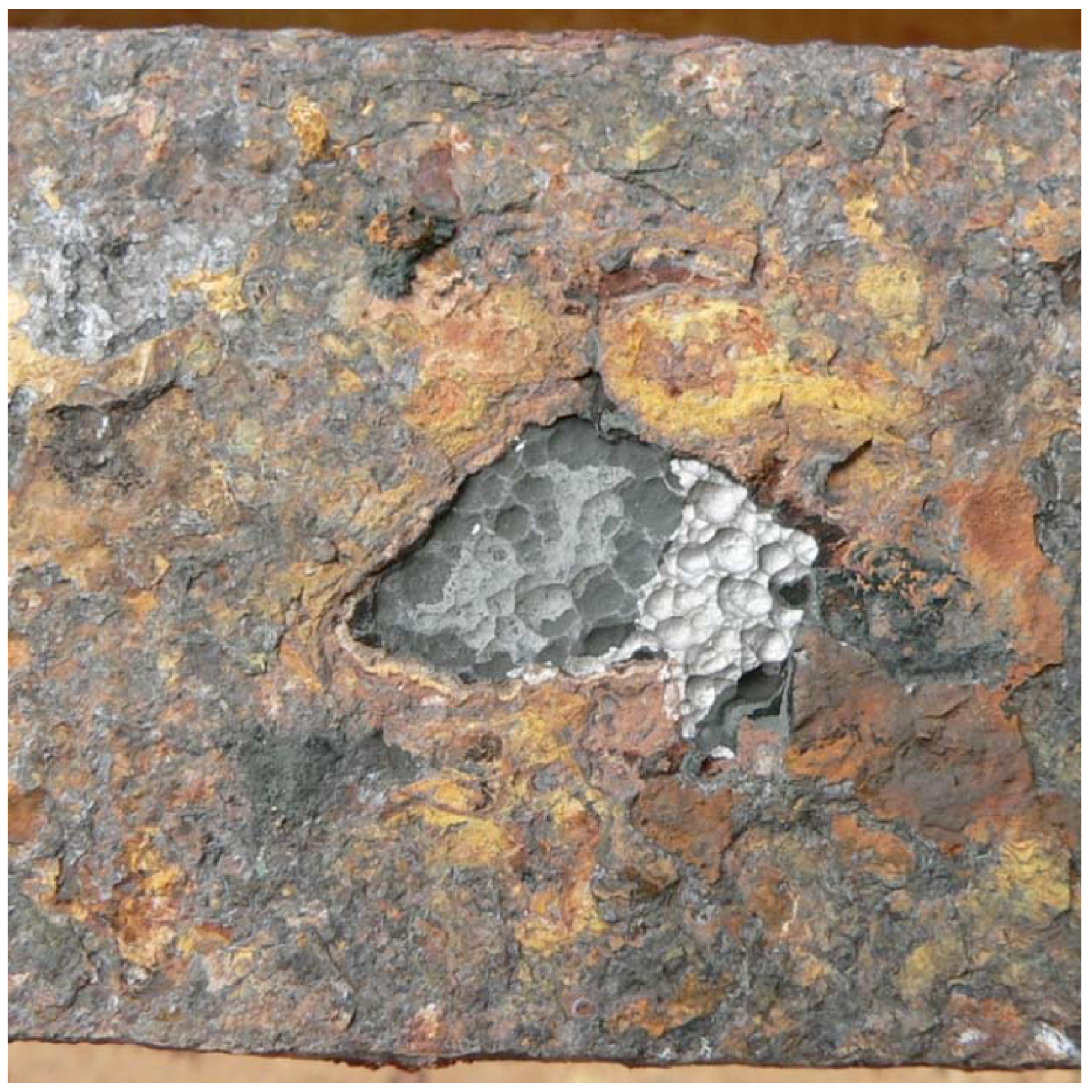
A number of observations made over a number of years of the corrosion products and their relation to the underlying steel, not previously reported, can be given meaning when viewed in terms of the propositions given above. For example, vertical steel strips exposed to immersion and tidal corrosion [51] showed overall corrosion products, but when sharply struck mechanically, revealed concentrated, localized areas of bright steel showing a dimpled pattern consistent with the rounded bottoms of groups of pits (Figure 10d). These areas were roughly circular and occupied only a small proportion of the total metal surface, most of which was covered with very adherent rusts. In some cases (e.g., Figure 12), part of the area from which the rusts had been removed by mechanical impact also showed a black area, which when closely examined, was very thin and followed the dimpled surface underneath. The whole area oxidized within 1–2 h of exposure, an insufficient time to obtain the composition using techniques such as X-ray diffraction (XRD) or Raman spectroscopy. There was no evidence of hydrogen sulphide odour immediately after uncovering the bright steel area, supporting the notion that the black material was not FeS or a similar product from corrosion involving microbiologically-influenced corrosion through sulphate-reducing bacteria [52].
Closer examination of the sample in Figure 12 shows that the black layer extends under the brown rusts at the left edge of the bright steel zone. This is consistent with the notion that (oxygen-poor) magnetite underlies rusts that are more oxygenated and that magnetite lies immediately adjacent to the metal where there is no pitting (Figure 10e). However, this would not have been the case over the bright metal where it would be expected, on the basis of Figure 10c,d, that the magnetite is separated from the pit bases by electrolyte. Since this is a fluid with no structural strength, the magnetite will not be adherent to the steel and instead would have come away with the overlying rusts removed by the mechanical impact. Indeed, examination of the fragments of the removed rusts indicated that this was the case.
A number of other examples, generally similar to Figure 12, were obtained in the same experiment for different steel strips and for different elevations in the water column (Jeffrey and Melchers, 2009). Similar results were obtained, for example, for steel coupons recovered after four years of exposure in a tropical marine atmospheric environment. In these cases, too, bright dimpled metallic surface areas were revealed, surrounded by areas covered with adherent rusts. Often, there are also some areas with a green tinge, dimpled, adjacent to the bright steel, probably the so-called ‘green rusts’, known to be a transitory rust product [50]. From this, it appears likely that Figure 12 is not specific to one particular exposure condition.
Much less information is available for other metals, but there are some observations of pits having formed inside plateaus for aluminium exposed for up to 20 years in seawater environments [53] and also for shorter term exposures (two years) for aluminium alloy in natural seawater [54]. There also are similar observations for pitting of aluminium alloys under artificially-accelerated saline corrosion conditions [55].
5. Discussion
The observations of the corrosion and the rusts shown in Figure 12 and elsewhere are considered to be entirely consistent with the mechanism of the development of the corrosion process through pitting shown, schematically, in Figure 10. They indicate that pits can coalesce, as has been shown earlier [28], but now with a plausible mechanism for this to occur and consistent with the observation of bright steel at the bottom of plateaus being the merging of the bottoms of clusters of adjacent pits (Figure 12). Such bright steel can be associated only with low pH conditions, recognized as characteristic of the bottoms of pits in pitting corrosion [22,26,40,41]. The regular pattern of the dimpled floors of the plateaus adds support to the notion of groups of pits amalgamating to form plateaus. As outlined in Figure 10, this requires lateral growth of pits, and this is consistent with the results and implications of theoretical modelling [44].
Overall, Figure 10 and Figure 12 add support for the development of plateaus from the amalgamation of individual, adjacent pits under essentially anoxic conditions. Once a plateau has been established, it is possible, still under anoxic conditions, for new pitting to occur since, at the local level, the corrosion processes are unable to distinguish between a virgin surface and a pre-corroded one; the only matter of importance are the conditions for the initiation and development of the pitting process.
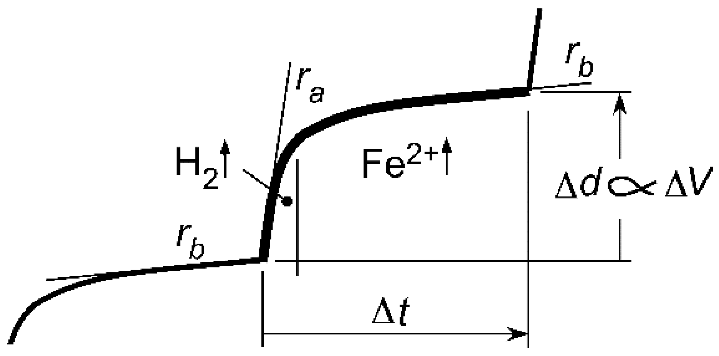
Gathering these strands together means that a continuous progression or cyclic pattern of repeated pitting can occur, within plateaus that then accommodate new pitting and that eventually combine to form a newer, deeper plateau than before. The basic component of this repeated cycle of pitting is shown schematically in Figure 13. It shows that pit depth increases by Δd over a time increment Δt. During the whole of the time increment Δt, new pits are being formed, increasing the overall mass loss, but by and large, not significantly changing the maximum depth of pitting. This depth is constrained by the potential limitation (i.e., by ΔV).
It follows from Figure 13 that the development of pitting corrosion over extended exposure periods is governed both by ΔV and by Δt. For a given exposure scenario, ΔV can be expected to remain relatively constant, and thus, the development of pitting and corrosion loss is governed largely by Δt. It depends on the total amount of ferrous material that needs to be removed to create the plateaus and also on the rate at which the metal is removed under the given potential. These factors largely are controlled by the rate of diffusion of species operating under cathodic control. It has been proposed earlier that these are oxygen for Mode 1 and hydrogen for Mode 2 and that the rates of diffusion depend on the thickness of the corrosion products, in particular that of magnetite [56].
In this context, it is noted that the process of cycling of pitting corrosion occurring under anoxic conditions differs in important ways from the initial cycle of pitting from first exposure, that is Mode 1 in Figure 1. In this mode, the process usually starts ab-initio from oxygen-rich conditions, with the rate limiting condition being the rate of oxygen arrival at the corroding surface, limited by the rate of diffusion of oxygen through the layers of corrosion products, reducing as these build-up, including the formation of the magnetite layer. For much of Mode 1, the instantaneous rate of corrosion is controlled primarily by the rate of inward diffusion of oxygen through the rust layer that builds up as corrosion progresses [6,56]. Since a build-up of corrosion products is required, the time required for the pitting processes to achieve a pit plateau will take considerably longer in Mode 1 than for the earlier cycles in Mode 2 when hydrogen is involved. This time difference gives rise to the bi-modal characteristic. The rust layer that develops during corrosion in Mode 1 is known to become non-homogeneous with depth and to be denser and less permeable closer to the metal surface. Magnetite invariably is the inner layer of rusts [48]. When the rusts have developed sufficiently, the magnetite layer will be the main barrier to oxygen transportation inwards, that is up to time ta. It also will be the main barrier in the early part of Mode 2, but now for the corrosion rate controlled by outward hydrogen transportation. The latter is consistent with experimental observations (e.g., [57]). A mechanism for this has been proposed [56].
The severity of pitting, and thus also corrosion loss, in a given time period depends much on ΔV (Figure 13). One factor to affect ΔV is that of microbiological corrosion effects. Laboratory-based experimental work using artificially high nutrient loadings and mainly pure bacterial cultures has shown that severe corrosion, particularly pitting corrosion, can result from these conditions [52]. As part of that process, the bacteria are considered to provide the abiotic metabolites that increase the corrosion potential [56]. Further, it has been demonstrated, empirically, that elevated nutrient concentrations, causing increased corrosion of steels in seawater, have their main effect during the early part of Mode 2 (Phase 3) and also that they increase the long-term corrosion in Phase 4 (Figure 1), at least for up to about 15–20 years [35]. In terms of the mechanisms outlined herein, it can be inferred that, as a result of microbiological activity, the increment in pit depth Δp in Figure 12 will be increased, as a consequence of the increase in the electrochemical potential ΔV set up by metabolites. Further verification and quantification of this effect would be desirable, but the principles appear to be clear.
Somewhat similar comments are likely to apply for the effect of chloride ion concentration. Natural chloride concentrations are very similar for most seawaters, but for these and for freshwaters, increasing the chloride concentration would be expected to increase the severity of pitting corrosion. The principles for this are well established [58]. Even in natural waters, the effect can be seen by comparing the data for pit depths observed on steels exposed in the Panama Canal Zone to seawater as compare with those exposed to fresh water [20].
The observations given above do call into question the applicability of electrochemical techniques in the study of longer term pitting and in particular the use of applied potentials to speed up the corrosion process. Since the depth of pitting, such as in the natural environments considered herein, is constrained by the potential drop through the pit, potential applied to increase the rate of corrosion also will increase the potential for pitting and thus lead to deeper pits, deeper than would be expected under natural conditions. In the limit, the plateauing effect would be bypassed and the cyclic nature of pitting lost. The imitations of electrochemical techniques in this regard are well known [59] and have been demonstrated by comparing field studies with electrochemical observations [60].
Particularly for longer term observations with observation points at intervals of several years, any observation of the depths of the pits at a particular time point constitutes very much a ‘snap-shot’ of the development of pit depths to that point in time. Unlike the idealized behaviour shown in Figure 6, in most scenarios, it would be expected that pit depths would be at various stages in the cycle of pitting (Figure 13). In addition, in practice, there will be small variations in ΔV and in Δt, but likely to be far more important is the accumulated effect of such variations over the exposure period. The latter is likely to produce a corrosion pattern in which the developments of pits over the surface are not in sequence, in part owing to delayed commencement of pit initiation and in part due to slightly different rates of pit growth. The net effect is the apparent randomness often associated with pit depths, particularly at longer exposure times. Because of these factors, it is permissible, in the limit (i.e., asymptotically), to consider pit depths as statistically independent variable ‘realizations’ [61]. Such independence is an important theoretical requirement for the proper application of extreme value theory, including to pit depth data [62]. In turn, this is necessary for maximum pit depth predictions and associated probabilities of occurrence to have both fundamental and empirical validity for practical applications.
Finally, a proposition can be offered for the overall development of pit depth with time, and the observations that it tends to follow a pattern similar to general corrosion as derived from mass loss, even for mild and low alloy steels (Figure 5). As noted, for the early part of the process (Mode 1, Figure 1), oxygen-rich conditions exist, and the rate of pitting is controlled by the rate of inwards oxygen diffusion that slows as the rust layers build-up. In the early part of Mode 2 (Phase 3, Figure 1), the potential for pitting will be adjusted slightly to match the change from oxygen to hydrogen in the cathodic reaction, theoretically [56] and also observed in pit depth data [63]. However, the change from the rate of the cathodic reaction being governed by oxygen diffusion to hydrogen diffusion means the time increment Δt becomes much shorter, leading to a considerable increase in the rate at which pit depth develops. Eventually, however, the further build-up of corrosion products also will reduce the rate of outward hydrogen diffusion [56], lengthening the time increments Δt and slowing the rate at which pit depth develops, on average. This proposition appears plausible. It can be used as a basis for further investigations to ascertain its validity.
6. Concluding Remarks
Collecting together various observations from diverse parts of the literature, it is possible to give explanations for the development of pitting corrosion in the slightly alkaline seawater marine environment. The principal features of such development are:
- After initiation and reaching stable growth, pits will continue to grow in depth until the potential driving the growth in pit depth becomes exhausted as pit depth increases. However, this still permits lateral growth of the pits, and eventually, this may result in pit coalescence with neighbouring pits to form plateaus of relatively uniform depth. These are sometimes known as broad pits.
- Observational data indicate that new pits form on the floors of the broad pits, particularly in low pH anoxic conditions such as under the magnetite corrosion product layer. In turn, this can lead to a new cycle of pit coalescence and the formation of deeper broad pits. The result is that the pitting growth behaviour can be considered episodic rather than a continued smooth growth in depth, as commonly assumed.
- Since not all points on a surface where anodic dissolution occurs are subject to exactly the same potential differences, pit development will vary from point to point on the surface and can be considered, asymptotically, to have pit depths that are statically independent. This allows valid application of extreme value analysis to the depth of pitting, as has been done for many years, but on an empirical basis.
- The model for pit depth development proposed herein also allows rational explanations for the effects of chlorides and of microbiological influences on pit depth. It also provides a basis for relating pit depth development to overall general corrosion loss development, even for mild and low alloys steels.
Funding
This research received funding from the Australian Research Council under grant DP140103388.
Conflicts of Interest
The authors declare no conflict of interest.
References
- Dankiw, R. Structural corrosion issues on Collins class submarines. In Proceedings of the Conference on Corrosion and Protection, Australasian Corrosion Association, Melbourne, Australia, 19–22 November 2006; p. 63. [Google Scholar]
- Mart, P.; Moore, B.; Martin, B.; Christopoulos, T.; Gage, N. Corrosion investigations of RAN minehunters. In Proceedings of the Conference Corrosion and Protection, Australasian Corrosion Association, Melbourne, Australia, 20–23 November 2005; p. 73. [Google Scholar]
- Bai, Y.; Bai, Q. Subsea Pipelines and Risers; Elsevier: Oxford, UK, 2012. [Google Scholar]
- Lee, T.M.; Melchers, R.E.; Beech, I.B.; Potts, A.E.; Kilner, A.A. Microbiologically influenced corrosion (MIC) of mooring systems: Diagnostic techniques to improve mooring integrity. In Proceedings of the 20th Offshore Symposium, Houston, TX, USA, 17 February 2015. [Google Scholar]
- Melchers, R.E. The effect of corrosion on the structural reliability of steel offshore structures. Corros. Sci. 2005, 47, 2391–2410. [Google Scholar] [CrossRef]
- Melchers, R.E. Modeling of marine immersion corrosion for mild and low alloy steels—Part 1: Phenomenological model. Corrosion 2003, 59, 319–334. [Google Scholar] [CrossRef]
- Melchers, R.E.; Jeffrey, R. The critical involvement of anaerobic bacterial activity in modelling the corrosion behaviour of mild steel in marine environments. Electrochim. Acta 2008, 54, 80–85. [Google Scholar] [CrossRef]
- Melchers, R.E. Bi-modal trend in the long-term corrosion of aluminium alloys. Corros. Sci. 2014, 82, 239–247. [Google Scholar] [CrossRef]
- Melchers, R.E. Bi-modal trends in the long-term corrosion of copper and copper alloys. Corros. Sci. 2015, 95, 51–61. [Google Scholar] [CrossRef]
- Petersen, R.B.; Melchers, R.E. Bi-modal trending for corrosion loss of steels buried in soils. Corros. Sci. 2018, 137, 194–203. [Google Scholar] [CrossRef]
- Tammann, G. Lehrbuch der Metallographie, 2nd ed.; Leopold Voss: Leipzig, Germany, 1932. [Google Scholar]
- Booth, F. A note on the theory of surface diffusion reactions. Trans. Faraday Soc. 1948, 44, 796–801. [Google Scholar] [CrossRef]
- Evans, U.R. The Corrosion and Oxidation of Metals: Scientific Principles and Practical Applications; Edward Arnold: London, UK, 1960. [Google Scholar]
- Melchers, R.E. Mathematical modelling of the diffusion controlled phase in marine immersion corrosion of mild steel. Corros. Sci. 2003, 45, 923–940. [Google Scholar] [CrossRef]
- King, F.; Lilja, C.; Vähänen, M. Progress in the understanding of the long-term corrosion behaviour of copper canisters. J. Nucl. Mater. 2013, 438, 228–237. [Google Scholar] [CrossRef]
- Melchers, R.E. Effect of small compositional changes on marine immersion corrosion of low alloy steel. Corros. Sci. 2004, 46, 1669–1691. [Google Scholar] [CrossRef]
- Melchers, R.E. Effect on marine immersion corrosion of carbon content of low alloy steels. Corros. Sci. 2003, 45, 2609–2625. [Google Scholar] [CrossRef]
- Melchers, R.E. Long-term corrosion of cast irons and steel in marine and atmospheric environments. Corros. Sci. 2013, 68, 186–194. [Google Scholar] [CrossRef]
- Melchers, R.E. Pitting corrosion of mild steel in marine immersion environment—1: Maximum pit depth. Corrosion 2004, 60, 824–836. [Google Scholar] [CrossRef]
- Forgeson, B.W.; Southwell, C.R.; Alexander, A.L. Corrosion of metals in tropical environments—Part 3—Underwater corrosion of ten structural steels. Corrosion 1960, 16, 87–96. [Google Scholar] [CrossRef]
- Burstein, G.T.; Pistorius, P.C.; Mattin, S.P. The nucleation and growth of corrosion pits on stainless steels. Corros. Sci. 1993, 35, 57–62. [Google Scholar] [CrossRef]
- Fontana, M.G.; Greene, N.D. Corrosion Engineering; McGraw-Hill Book Co.: New York, NY, USA, 1967. [Google Scholar]
- Butler, G.; Stretton, P.; Beynon, J.G. Initiation and growth of pits on high-purity iron and its alloys with chromium and copper in neutral chloride solutions. Br. Corros. J. 1972, 7, 168–173. [Google Scholar] [CrossRef]
- Mercer, A.D.; Lumbard, E.A. Corrosion of mild steel in water. Br. Corros. J. 1995, 30, 43–55. [Google Scholar] [CrossRef]
- Pourbaix, M. Significance of protection potential in pitting and intergranular corrosion. Corrosion 1970, 26, 431–438. [Google Scholar] [CrossRef]
- Wranglen, G. Pitting and sulphide inclusions in steel. Corros. Sci. 1974, 14, 331–349. [Google Scholar] [CrossRef]
- Frankel, G.S.; Li, T.; Scully, J.R. Perspective—Localized corrosion: Passive film breakdown vs pit growth stability. J. Electrochem. Soc. 2017, 164, C180–C181. [Google Scholar] [CrossRef]
- Jeffrey, R.; Melchers, R.E. The changing topography of corroding mild steel surfaces in seawater. Corros. Sci. 2007, 49, 2270–2288. [Google Scholar] [CrossRef]
- Asadi, Z.S.; Melchers, R.E. Pitting corrosion of older underground cast iron pipe. Corros. Eng. Sci. Technol. 2017, 52, 459–469. [Google Scholar] [CrossRef]
- Melchers, R.E. Modeling of marine immersion corrosion for mild and low alloy steels—Part 2: Uncertainty estimation. Corrosion 2003, 59, 335–344. [Google Scholar] [CrossRef]
- Melchers, R.E.; Ahammed, M. Statistical characterization of corroded steel plate surfaces. J. Adv. Struct. Eng. 2006, 9, 83–90. [Google Scholar] [CrossRef]
- Melchers, R.E. Pitting corrosion of mild steel in marine immersion environment—2: Variability of maximum pit depth. Corrosion 2004, 60, 937–944. [Google Scholar] [CrossRef]
- Blekkenhorst, F.; Ferrari, G.M.; van der Wekken, C.J.; IJsseling, F.P. Development of high strength low alloy steels for marine applications, Part 1: Results of long term exposure tests on commercially available and experimental steels. Br. Corros. J. 1986, 21, 163–176. [Google Scholar] [CrossRef]
- OSPAR, Regional Quality Status Report II for the Greater North Sea. OSPAR Commission for the Protection of the Marine Environment of the North-East Atlantic. 2000. Available online: http://www.ospar.org/eng/html/qsr2000 (accessed on 29 June 2018).
- Melchers, R.E. Long-term immersion corrosion of steels in seawaters with elevated nutrient concentration. Corros. Sci. 2014, 81, 110–116. [Google Scholar] [CrossRef]
- Fontaine, E.; Rosen, J.; Potts, A.; Ma, K.-T.; Melchers, R.E. Feedback on MIC and pitting corrosion from field recovered mooring chain links. In Proceedings of the Offshore Technology Conference, Houston, TX, USA, 5–8 May 2014. [Google Scholar]
- Chaves, I.A.; Melchers, R.E. Pitting corrosion in pipeline steel weld zones. Corros. Sci. 2011, 53, 4026–4032. [Google Scholar] [CrossRef]
- de la Fuente, D.; Otero-Huerta, E.; Morcillo, M. Studies of long-term weathering of aluminium in the atmosphere. Corros. Sci. 2007, 49, 3134–3148. [Google Scholar] [CrossRef] [Green Version]
- Vargel, C. Corrosion of Aluminium; Elsevier: London, UK, 2004. [Google Scholar]
- Szklarska-Smialowska, Z.S. Pitting Corrosion of Metals; National Association of Corrosion Engineers: Houston, TX, USA, 1986. [Google Scholar]
- Frankel, G.S. Pitting corrosion of metals a review of the critical factors. J. Electrochem. Soc. 1998, 145, 2186–2198. [Google Scholar] [CrossRef]
- Galvele, J.R. Transport processes and the mechanism of pitting of metals. J. Electrochem. Soc. 1976, 123, 464–474. [Google Scholar] [CrossRef]
- Pickering, H.W. Important early developments and current understanding of the IR mechanism of localized corrosion. J. Electrochem. Soc. 2003, 150, K1–K13. [Google Scholar] [CrossRef]
- Sharland, S.M.; Tasker, P.W. A mathematical model of crevice and pitting corrosion—I. The physical model. Corros. Sci. 1988, 28, 603–620. [Google Scholar] [CrossRef]
- Turnbull, A. A review of modelling of pit propagation kinetics. Br. Corr. J. 1993, 28, 297–308. [Google Scholar] [CrossRef]
- Alavi, A.; Cottis, R.A. The determination of pH, potential and chloride concentration in corroding crevices on 304 stainless steels and 7475 aluminium ally. Corros. Sci. 1987, 27, 443–451. [Google Scholar] [CrossRef]
- Phull, B.S.; Pikul, S.J.; Kain, R.M. Seawater corrosivity around the world—Results from five years of testing. In Corrosion Testing in Natural Waters, 2nd ed.; Kain, R.M., Young, W.T., Eds.; ASTM: West Conshohocken, PA, USA, 1997; pp. 34–73. [Google Scholar]
- Evans, U.R.; Taylor, C.A.J. Mechanism of atmospheric rusting. Corros. Sci. 1972, 12, 227–246. [Google Scholar] [CrossRef]
- Stratmann, M.; Muller, J. The mechanism of the oxygen reduction on rust-covered metal substrates. Corros. Sci. 1994, 36, 327–359. [Google Scholar] [CrossRef]
- Gilberg, M.R.; Seeley, N.J. The identity of compounds containing chloride ions in marine iron corrosion products: A critical review. Stud. Conserv. 1981, 26, 50–56. [Google Scholar]
- Jeffrey, R.; Melchers, R.E. Corrosion of vertical mild steel strips in seawater. Corros. Sci. 2009, 51, 2291–2297. [Google Scholar] [CrossRef]
- Little, B.J.; Lee, J. Microbiologically Influenced Corrosion; Wiley-Interscience: New York, NY, USA, 2007. [Google Scholar]
- Sun, S.; Zheng, Q.; Li, D.; Wen, J. Long-term atmospheric corrosion behaviour of aluminium alloys 2024 and 7075 in urban, coastal and industrial environments. Corros. Sci. 2009, 51, 719–727. [Google Scholar] [CrossRef]
- Liang, M.X.; Chaves, I.A.; Melchers, R.E. Corrosion and pitting of 6060 series aluminium after 2 years exposure in seawater splash, tidal and immersion zones. Corros. Sci. 2018, in press. [Google Scholar] [CrossRef]
- Li, H.; Garvan, M.R.; Li, J.; Echauz, J.; Brown, D.; Vachtsevanos, G.J. Imaging and information processing of pitting-corroded aluminum alloy panels with surface metrology methods. In Proceedings of the Annual Conference on Prognostics and Health Management Society, Fort Worth, TX, USA, 29 September–2 October 2014; ISBN 978-1-936263-17-2. [Google Scholar]
- Melchers, R.E. Microbiological and abiotic processes in modelling longer-term marine corrosion of steel. Bioelectrochemistry 2014, 97, 89–96. [Google Scholar] [CrossRef] [PubMed]
- Bargeron, C.B.; Benson, R.C. Analysis of the gases evolved during the pitting corrosion of aluminum in various electrolytes. J. Electrochem. Soc. 1980, 127, 2528–2530. [Google Scholar] [CrossRef]
- Jones, D.A. Principles and Prevention of Corrosion, 2nd ed.; Prentice-Hall: Upper Saddle River, NJ, USA, 1996. [Google Scholar]
- Kelly, R.G.; Scully, J.R.; Shoesmith, D.; Buchheit, R.G. Electrochemical Techniques in Corrosion Science and Engineering; Marcel Dekker: New York, NY, USA, 2003. [Google Scholar]
- Stockert, L.; Haas, M.; Jeffrey, R.J.; Melchers, R.E. Electrochemical measurements and short-term-in-situ exposure testing. In Proceedings of the Corrosion & Prevention 2012, Melbourne, Australia, 11–14 November 2012; p. 100. [Google Scholar]
- Leadbetter, M.R.; Lindgren, G.; Rootzen, H. Extremes and Related Properties of Random Sequences and Processes; Springer: New York, NY, USA, 1983. [Google Scholar]
- Galambos, J. The Asymptotic Theory of Extreme Order Statistics, 2nd ed.; Krieger: Malabar, FL, USA, 1987. [Google Scholar]
- Melchers, R.E.; Ahammed, M. Maximum pit depth variability in water injection pipelines. In Proceedings of the Conference on Internernational Society of Offshore Polar Engineer, (ISOPE2018), Sapporo, Japan, 10–15 June 2018; Volume 4, pp. 289–294. [Google Scholar]
Figure 1.
Schematic bi-modal model for long-term corrosion loss (from mass loss) showing the two modes, the various phases and some of the model parameters. In the idealized case, the change from predominantly oxic Mode 1 to predominantly anoxic Mode 2 occurs at ta with a change of the instantaneous corrosion rate from rb to ra.

Figure 2.
Rims of corrosion plateaus and pits at the base of the deepest plateau, as observed for mild steel exposed for about 12 months in temperate seawater (Jeffrey and Melchers [28]).
Figure 2.
Rims of corrosion plateaus and pits at the base of the deepest plateau, as observed for mild steel exposed for about 12 months in temperate seawater (Jeffrey and Melchers [28]).

Figure 3.
Data and trends for immersion corrosion of mild steel rotating coupons exposed in laboratory triply-distilled water at 70 °C and 0.4 ppm O2: (a) mass-loss, (b) depth of pits and (c) number of pits per unit area (data, but not the interpretations or trends, from Mercer and Lumbard [24]).
Figure 3.
Data and trends for immersion corrosion of mild steel rotating coupons exposed in laboratory triply-distilled water at 70 °C and 0.4 ppm O2: (a) mass-loss, (b) depth of pits and (c) number of pits per unit area (data, but not the interpretations or trends, from Mercer and Lumbard [24]).

Figure 4.
Pit depth data as in Figure 3b interpreted as stepped development of the depth of pitting.
Figure 4.
Pit depth data as in Figure 3b interpreted as stepped development of the depth of pitting.

Figure 5.
Data and trends for natural seawater immersion corrosion as a function of exposure time for mild steel exposed at Taylors Beach: (Figure 5) mass loss and (Figure 6) maximum pit depth, as well as the best-fit trends through the data sets.

Figure 6.
Same data as in Figure 5, but interpreted as stepped increments in the maximum depth of pits. The data suggest all increments are about 0.35 mm.
Figure 6.
Same data as in Figure 5, but interpreted as stepped increments in the maximum depth of pits. The data suggest all increments are about 0.35 mm.

Figure 7.
Data and trends for the maximum pit depth of three low alloy steels exposed to the North Sea, showing interpreted step-wise trending for pit depth development (data from Blekkenhorst et al. [33]).
Figure 7.
Data and trends for the maximum pit depth of three low alloy steels exposed to the North Sea, showing interpreted step-wise trending for pit depth development (data from Blekkenhorst et al. [33]).

Figure 8.
Data for pit depth in the heat-affected zone of the pipe weld region with added interpreted step-wise trending (data from [37]).
Figure 8.
Data for pit depth in the heat-affected zone of the pipe weld region with added interpreted step-wise trending (data from [37]).

Figure 9.
Data and trend for mass loss of 99% (wt) pure aluminium exposed to a marine atmosphere at Bilbao, together with schematic trend for deepest pits and for maximum pit depth (data from [38]).
Figure 9.
Data and trend for mass loss of 99% (wt) pure aluminium exposed to a marine atmosphere at Bilbao, together with schematic trend for deepest pits and for maximum pit depth (data from [38]).

Figure 10.
Schematic representation of the sequence in pit depth development.
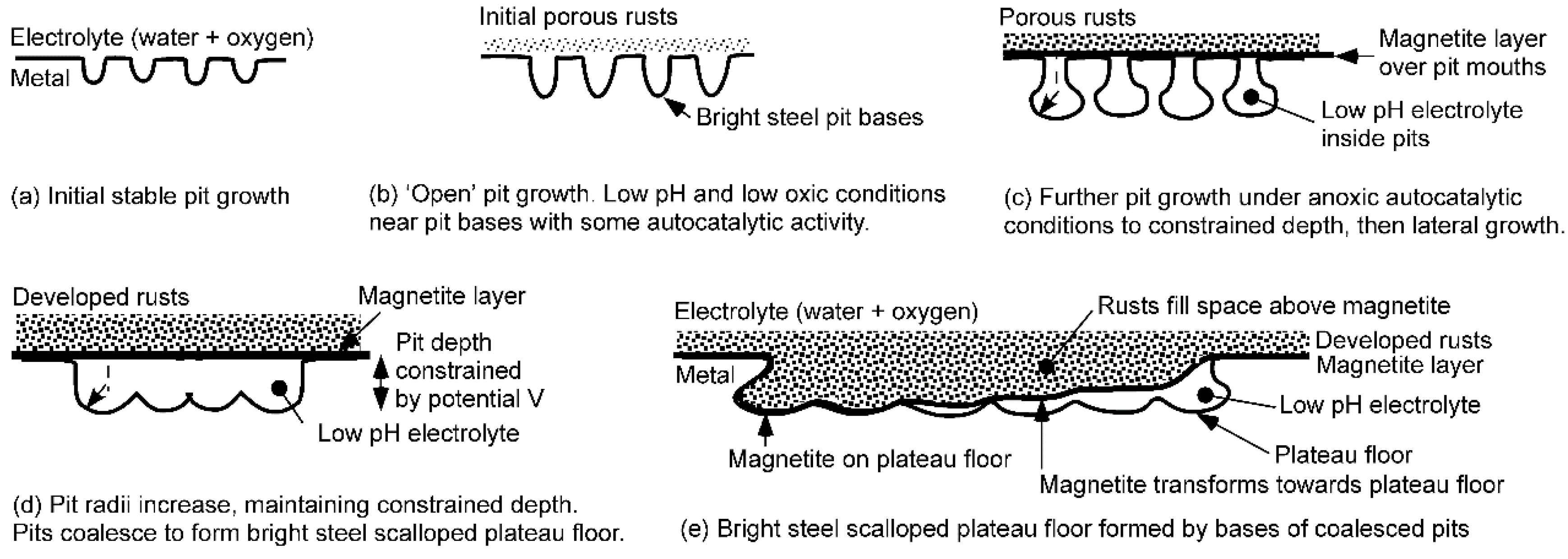
Figure 11.
Mild steel showing corrosion product (rust) and its local rupture over pit mouths, after 12 months of exposure at Taylors Beach (bar = 20 microns).
Figure 11.
Mild steel showing corrosion product (rust) and its local rupture over pit mouths, after 12 months of exposure at Taylors Beach (bar = 20 microns).
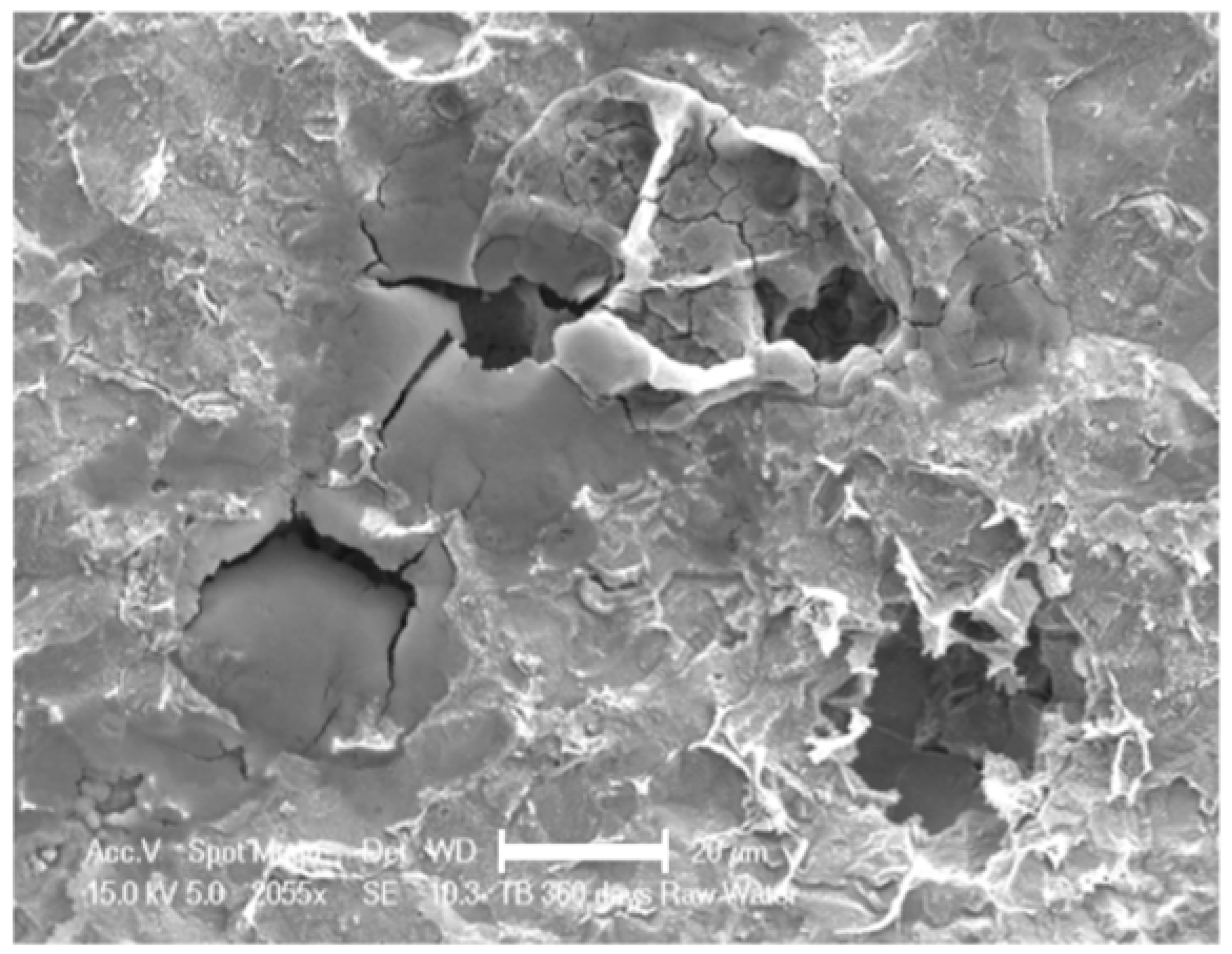
Figure 12.
Broad pit revealed after removal of loose rusts by mechanical impact. Dimpled bright steel at the floor of the plateau partly covered with (dark/black) magnetite. The whole area oxidized within 1–2 h after exposure.
Figure 12.
Broad pit revealed after removal of loose rusts by mechanical impact. Dimpled bright steel at the floor of the plateau partly covered with (dark/black) magnetite. The whole area oxidized within 1–2 h after exposure.

Figure 13.
One cycle of pitting under internally anoxic conditions showing pit depth increment Δd for time increment Δt. Furthermore, ΔV is the electrochemical potential driving the depth of the pit increment.
Figure 13.
One cycle of pitting under internally anoxic conditions showing pit depth increment Δd for time increment Δt. Furthermore, ΔV is the electrochemical potential driving the depth of the pit increment.
© 2018 by the author. Licensee MDPI, Basel, Switzerland. This article is an open access article distributed under the terms and conditions of the Creative Commons Attribution (CC BY) license (http://creativecommons.org/licenses/by/4.0/).
Share and Cite
MDPI and ACS Style
Melchers, R.E. A Review of Trends for Corrosion Loss and Pit Depth in Longer-Term Exposures. Corros. Mater. Degrad. 2020, 1, 42-58. https://doi.org/10.3390/cmd1010004
AMA Style
Melchers RE. A Review of Trends for Corrosion Loss and Pit Depth in Longer-Term Exposures. Corrosion and Materials Degradation. 2020; 1(1):42-58. https://doi.org/10.3390/cmd1010004
Chicago/Turabian StyleMelchers, Robert E. 2020. "A Review of Trends for Corrosion Loss and Pit Depth in Longer-Term Exposures" Corrosion and Materials Degradation 1, no. 1: 42-58. https://doi.org/10.3390/cmd1010004