Azimuthal Fermionic Current in the Cosmic String Spacetime Induced by a Magnetic Tube
by
Mikael Souto Maior de Sousa
1,†, 
Rubens Freire Ribeiro
2,† and
Eugênio Ramos Bezerra de Mello
2,*,† 1
Centro de Educação, CAp, Universidade Federal de Roraima, Boa Vista 69304-000, Brazil
2
Departamento de Física; Universidade Federal da Paraíba, João Pessoa 58059-900, Brazil
*
Author to whom correspondence should be addressed.
†
These authors contributed equally to this work.
Particles 2018, 1(1), 82-96; https://doi.org/10.3390/particles1010006
Submission received: 23 January 2018
/
Revised: 12 March 2018
/
Accepted: 12 March 2018
/
Published: 16 March 2018
(This article belongs to the Special Issue Selected Papers from “The Modern Physics of Compact Stars and Relativistic Gravity 2017”)
Abstract
:In this paper, we calculate the vacuum expectation value of the azimuthal fermionic current, associated with a massive fermionic quantum field in the spacetime of an idealized cosmic string, considering the presence of a magnetic tube of radius a, coaxial to the string. In this analysis three distinct configurations of magnetic field are considered: (i) a magnetic field concentrated on a surface of the tube; (ii) a magnetic field presenting a radial dependence; and (iii) an homogeneous magnetic field. In order to develop this analysis , we construct the complete set of normalized solution of the Dirac equation in the region outside the tube. By using the mode-sum formula, we show that the azimuthal induced current is formed by two contributions: the first being the current induced by a line of magnetic flux running along the string, and the second, named core-induced current, is induced by the non-vanishing extension of the magnetic tube. The first contribution depends only on the fractional part of the ration of the magnetic flux inside the tube by the quantum one; as to the second contribution, it depends on the total magnetic flux. We specifically analyze the core-induced current in several limits of the parameters and distance to the tube.
1. Introduction
In 1957, A.A. Abrikosov [1], by using the Ginzburg-Landau superconductivity theory, showed that there exist a magnetic flux tube penetrating in a type II superconductor, that was named vortex, when the intensity of the field is bigger then the critical one, . Some years later, adopting a relativistic formalism, Nielsen and Olesen [2] have found vortex configurations, by using field theory, with Higgs field interacting with Abelian one. The numerical analysis of the influence of this system on the geometry of the spacetime was made in [3,4]. The authors have shown that, as in flat space, the system presents also cylindrically symmetric solutions, having a magnetic field of finite extension. They also shown that the space around the vortex is asymptotically Minkowski minus a wedge. Two length scales naturally appear in this formalism, the one related with the extension of the magnetic flux proportional to the inverse of vector field mass, , and the other associated with the inverse of the scalar field mass, , being the radius that the scalar field reaches its vacuum value.
In the analysis of the behavior of a quantum charged field in the neighborhood a (NO) string [2] one has to take into account the influence of the geometry of the spacetime and the presence of the magnetic field. In this way two different procedure can be adopted: The first one is to consider the vortex without inner structure, having a magnetic flux running along a straight line and the topology of the surface orthogonal to it been conical one. The second procedure is to consider this object having a non-vanishing core. The first approach the can be exactly solved; as to the second one, it is beyond our analytical comprehension. In the first approach, the idealized model, the periodicity condition imposed on the quantum field due to the conical topology leads to a modification of the spectrum of the zero-point fluctuations of quantized fields shifting the vacuum expectation values (VEV) for many physical quantities (see for instance references given in [5]). Considering the presence of the magnetic flux, additional polarization effects take place, these ones associated with charged quantum fields, as we can see in [6,7,8,9,10,11]. Specifically speaking the magnetic flux induces a non-zero azimuthal current densities, (see references [12,13]). Although the results found for these currents are calculated considering a fixed configuration of magnetic field, these currents act as sources of the semiclassical Maxwell’s equations and play important roles in modeling a self-consistent dynamics involving the electromagnetic fields. In higher-dimensional cosmic string spacetime, the analysis of induced fermionic currents in the presence of a magnetic flux have can be seen in [14]. In all these analysis, the authors have shown that induced azimuthal vacuum current densities take place if the ratio of the magnetic flux by the quantum one has a nonzero fractional part. In fact, induced fermionic and scalar current densities in compactified cosmic string spacetimes have been considered in [15,16].
As it is well known, the analysis of a quantum system in a realistic model for the NO vortex cannot be exactly solvable, but an intermediate approach can be adopted. In this way, we consider the spacetime produced by the string as being conical everywhere, but having a non-zero thickness magnetic field surrounding it. This means that this model is valid in the case where the width of the string can be completely neglected, or similarly in the case where the size of the magnetic tube is much larger than the string width. In this way, some improvements may be obtained. In fact, in [17,18,19] this approach was used to calculate the VEV of massless charged scalar and fermionic energy-momentum tensors, , respectively. The scalar vacuum current induced by a magnetic flux in a cosmic string considering a non-vanishing core has been developed in [20]. In these calculations we see that the vacuum polarization effects were developed for the region outside the tube, and presented two contributions. The first one associated with a zero-thickness magnetic flux, and the second one induced by the non-vanishing core, called core-induced contributions. It is seen that the first contribution is a periodic function of the magnetic flux inside the tube, with the period equal to the quantum flux, , however the second contribution, in general, it is not periodic function of the quantum flux. In fact, the core-induced contributions depend on the total magnetic flux inside the core. This non-periodic function is the new one, and its analyses corresponds the main objective of this paper.
We organized this paper as follows. In Section 2 we provided the geometry associated with the cosmic string spacetime and the configurations of the magnetic fields adopted. Moreover we construct the set of normalized solutions of the Dirac equation in the region outside the core in a general formalism, that can be applied to each of the three configurations of magnetic field. In Section 2.1, we use the mode-summation method to calculate the induced azimuthal current density. We show that this current can be decomposed in two parts: The first one corresponds to idealizing cosmic string having a magnetic flux running along its core, and the second one is induced by the non-zero core of the magnetic tube. In Section 2.2, we discuss the core-induced azimuthal current in various asymptotic regions of the parameters. In Section 3 we present some plots associated with the core-induced azimuthal current exhibiting its behavior as function of the most relevant physical variables. Finally, our most relevant conclusions are summarized in Section 4.
2. The Geometry and the Fermionic Wave-Functions
The geometry of an idealized cosmic string along the z-axis, can described in cylindrical coordinate system, by the following line element:
In this system the coordinates take values in range , and . The conical structure of this spacetime is codified through the parameter . In fact, the parameter q depends on the linear mass density of the string, , by the relation .
In curved spacetime and in the presence of a electromagnetic four-vector potential, , we can describe the quantum dynamic of a massive charged spinor by the Dirac equation,
where the Dirac matrices in curved space-time are , and is the spin connection that generalize the spinor concept to derivative in curved spacetime. For this geometry the gamma matrices may be written in the form,
Here we have introduced the Pauli matrices in cylindric coordinates for :
To the four-vector potential we consider
being
Here in this analysis, we consider three different configurations of magnetic fields that allow as to solve the Dirac equation exactly. They are: (i) a magnetic field concentrated on a surface of the tube; (ii) a magnetic field presenting a radial dependence; and (iii) an homogeneous magnetic field. For these fields the function for the cylindrical magnetic shell is given by
While for the second (magnetic field as function of ) and third (constant magnetic field) configurations, the radial function reads,
with
Now, we present the procedure to obtain positive energy solution of Dirac equation. We assume the time-dependence of the eigenfunctions like and express the four-component spinor into the upper and lower components:
If we substitute the function from the (12) into the (11), we find a second order differential equation for the two-component spinor :
At this point let us assume that the general solutions to and can be express in terms of the cylindrical symmetry ansatz below,
where we used the compact notation .
We impose that this function must be eigenfunction of the total angular momentum along the string, ,
This imposition leads to
To construct the complete set of the wave-functions we will consider (13) in the regions and , separately. For the inner region, we have three different configurations of magnetic field given by (5)–(9), as we showed previously. For the outer region, , there is no magnetic field and the vector potential is given by,
Therefore, after some intermediate steps, we can express the external positive-energy solution of the Dirac equation by
with being an integer number. We have defined
where is the sign of , being and and and are the Bessel and Neumann functions respectively. Is verified a similar result for the lower components Dirac spinor. Notice that we have introduced a set of eight constants , , and with in the above general solution. As to the energy we have
given in terms of .
Using (11) and (12) we are able to find a relation between the constants of the the upper and lower solutions in (18). In addition, following Nail [21] we require the following relation:
with
Applying the above relations, and after some intermediates steps, we obtain
Henceforward, the positive energy exterior solutions for the Dirac equation, will be specified by the quantum numbers . It has the form
where the parameter is defined by
For the inner region, , we have three different configurations of magnetic field. Consequently, there will be three different solutions for (13). Let us define each radial function represented by , where we introduced , the index associated with the model and the index associated to the spinor components. For this region, , we have the positive-energy spinor field in the general form given by:
By the continuity condition imposed on the fermionic wave function at the boundary, it means , we can related the constants and , in (25), and , in (27). After some intermediate steps we have,
where
In (30) generalize the Bessel functions and . Using this notation we have all information about the inner structure of the magnetic field confined in the coefficient .
Therefore, by the normalization condition
may be obtained, in (31) the delta symbol on the right-hand side is compacted notation to the delta function for continuous quantum numbers , and the Kronecker delta for discrete ones being the spatial metric tensor part determinant. The integration over the radial coordinate should be realized in the range . In this case two different expressions for the wave function must be used. The function (27) for and (25) for . The integration over the inner region is finite, it means that the dominant contributions for comes from the integration in the outsider region. Evolving the integrals involving the cylindrical Bessel functions, we get
The above relation determines the normalization constant for the inner wave function.
To the obtention of the outsider negative-frequency fermionic wave function we can follow the same procedure to the outsider positive-frequency one. This way, the positive- and negative-energy wave functions may be specified by the complete set of quantum numbers . Finally, we have these functions given below:
where we introduce the notations,
and
After we find the negative-frequency wave function for the outsider region of the magnetic flux, i.e., for , we will use it for the further investigations of the vacuum azimuthal fermionic current density.
2.1. Induced Azimuthal Fermionic Current
By using the the mode sum method we can obtained the vacuum expectation value (VEV) of the fermionic current density operator, , as given below,
here the compact notation defined by
is used.
To the VEV of the azimuthal current density we have specifically,
In fact, by using (3), (4), (35) and (38) we get the following expression for the induced azimuthal current density in the outsider region of the magnetic tube, that is given by:
Developing the product of , we can separate the functions into two contributions, that one does not depend on the inner structure of the magnetic field from the other that does, this separation is written as a sum of two terms as shown below:
The first term in (43), , corresponds to the induced azimuthal current density in the geometry of an ideal string cosmic having a magnetic flux running along its core. It reads,
As to the second, , corresponds to the azimuthal current induced by the non-vanishing extension of the magnetic tube. the latter is given by
where with are the Hankel functions.
In [15] it was presented the explicit derivation to . Here we reproduce only the more relevant steps. In order to provide a more workable expression we use the identity below
Doing this, it is possible to develop the integral over in (44), by using the results presented in [22]. Moreover, defining a new variable , we get
Being a new function obtained by a long manipulation over the summation on the quantum number j. It reads
and
where is the modified Bessel function of the first kind. The parameter corresponds to the fractional part of the ratio of the total magnetic flux by the quantum one, as showed below
with being an integer number. So we conclude that (47) is an odd function of .
For , the last term on the right-hand side of Equation (51) is absent.
Finally substituting the above results into (47), and after the integration over y, the expression (47) is presented in the form
In the above expression is the modified Bessel function of the second kind, and
The expression (53) depends on , and vanishes for . Therefore, we can say that is another kind of manifestation of the Aharonov-Bohm effect.
Now let us focus on the core-induced current . In order to present a more workable expression to (45), in the complex plane we rotate the integrals by the term for and respectively. For the coefficient that carrying the dependence of the specific configurations of the magnetic field, presented in (30), we can show that by the rotation on the complex plane we get the following relation,
developing the integration after the rotations is easy to see that over the segments occurs a mutual cancellation. Proceeding with the remaining integration over the imaginary axis we have introduce the modified Bessel functions. Making the variable substitution , the azimuthal current reads,
here we present the notation
After a some appropriate coordinate transformations in (56) we have:
2.2. Analytical Development
At this point to reinforce our calculations we will evaluate (58) for some asymptotic conditions. First we now evaluate the core-induced azimuthal current for large distances of the magnetic field structure. However, to do so we first consider massive fermionic fields in the large distances, it means, . In this case we assume that in (58) may be expressed its corresponding asymptotic form. This way, the induced current density may be presented as
The leading contribution for this integral is on the region near the lower limit of integration. This way we can approximated the asymptotic behavior for the massive case at large distances as follow,
The behavior of the term decays as for ; in consequence the latter dominates the total azimuthal current at large distances.
For massless fields in the limit . We will use the radial functions in the inner region of the magnetic structure. In [24,25] we provided exact solutions for and for the three different configurations of magnetic field. They are:
- For magnetic field concentrated on the surface of the tube:where , with .
- For the magnetic field as function of :whereand
- For the homogeneous magnetic field:where and are given by where and are given bywith
Where we can see that the second and third configurations, are expressed by the Whittaker functions, [22].
Now we will develop the behavior of the induced current at the limit for the massless fermionic fields. Expanding the (58) in powers of and keeping just the dominant contributions, given by the smaller power of the ratio . After intermediate steps, we get:
where
and for specifies de configuration of magnetic field that is adopted, given in [24]. In fact, this parameter depends on the intensity of the magnetic field. In fact, by (68) we can see that for the three configurations of magnetic field considered, the fermionic current density that is induced by the combination of the geometry spacetime and magnetic field structure decays with, , for large distance from the magnetic structure. In [15] is showed that for massless fields the zero-thickness azimuthal current decays with . This way, at this limit taken (43), is dominated by the zero-thickness contribution.
The next analyses is the behavior of near the boundary, it means, near the three configurations cylindrical magnetic field structure, that we will investigate separately. Actually next to this region the current diverges. To find the more relevant term we can introduce a new variable transformation, , in (58). It means that for the large order for the modified Bessel functions [26] we can use the uniform expansion, this way, after some steps, we have
in the above equation and . By the using of the approximation and taking into account that the denominator of the integrand in (70) can be approximate to unity, for the three configurations, we have:
Developing the above integral we have
where we notice that the current density diverges next to the boundary.
It is seen that has a finite value next to the boundary. Therefore, we conclude that, in this region, the total azimuthal current, (43) is dominated by the core-induced contribution.
3. Numerical Results
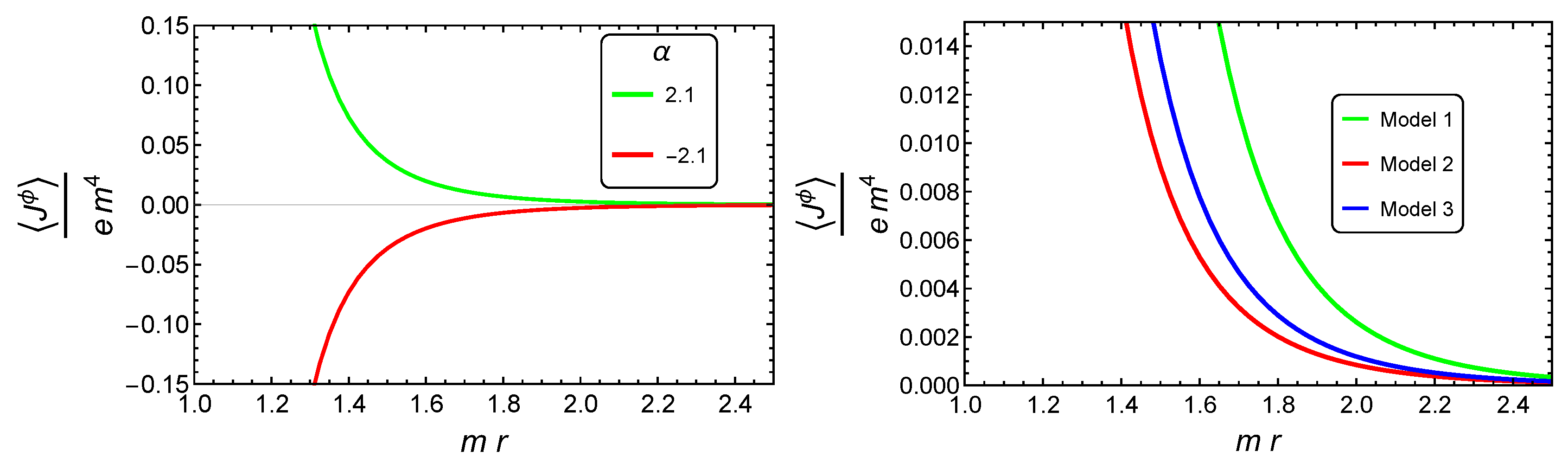
An analytical analysis has been developed in the previous section providing some pertinent informations about the behavior of ; however, it is limited and some further information about the core-induced fermionic current can be better understood with numerical analysis. Therefore, this section is devoted to provide these additional informations. In this way, we can see in Figure 1 the dependence of the induced current density as function of considering and . The left panel exhibits the dependence of with in units of considering the first configuration of magnetic field. In the latter is assumed two distinct values for . This plot also shows that the sign of the azimuthal current changes when we change the direction of the magnetic field. Another point that we wanted to investigate is about the influence of a specific configuration of the magnetic field on the intensity of the induced current. The answer to this question can be provided in the right panel. By this plot we may infer that the first model provide the current with biggest intensity. Finally as a general observation for both plots, we can affirm that near the core, , the intensities of the current become very high, and they decay very fast for , for massive fermionic field.
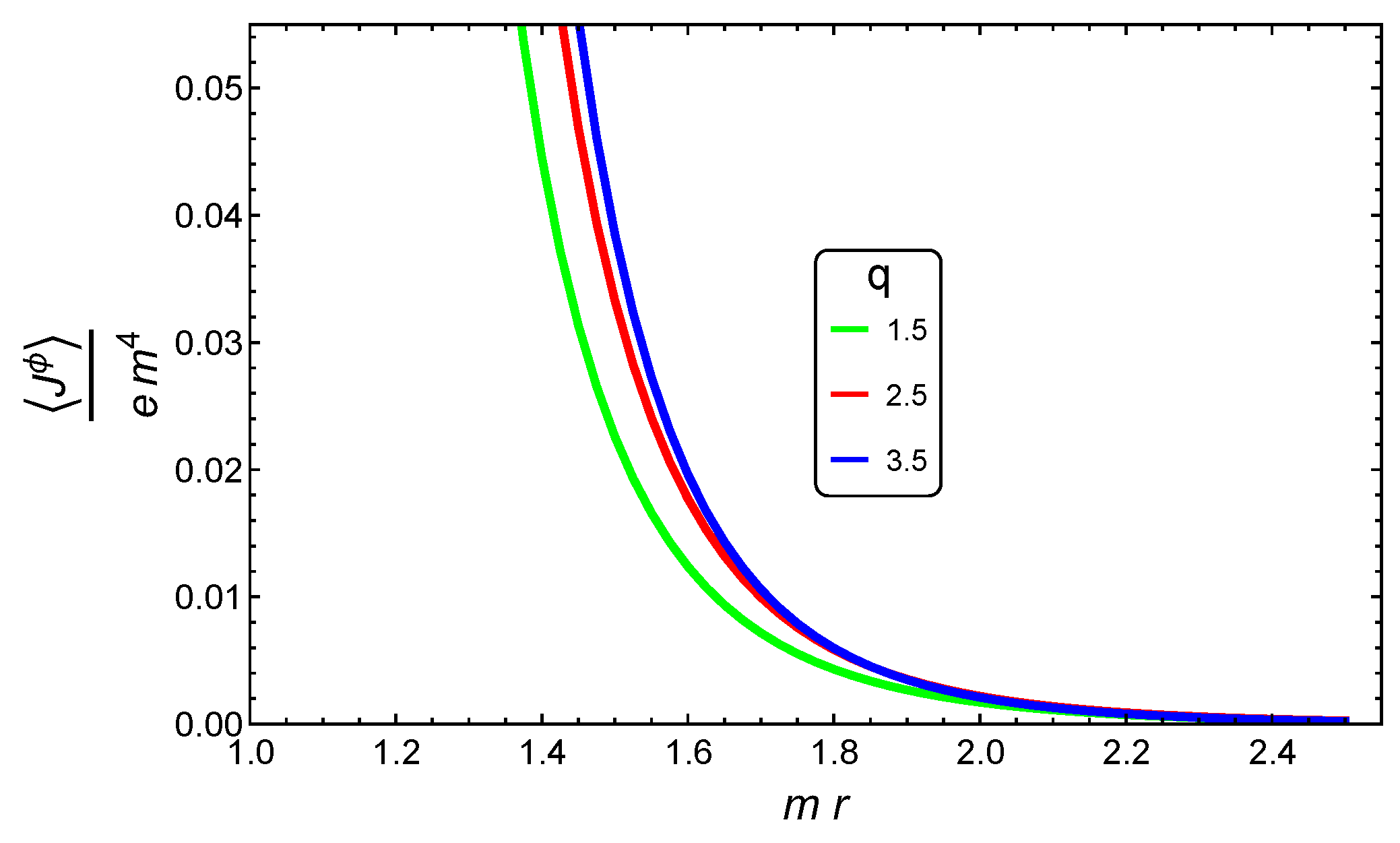
Anther point that we wanted to investigate is about the influence of the parameter q on the intensity of . In order to do that we display in Figure 2, the behavior of this current in units of , as function of , considering and . In this plot we have only considered the of the first configuration of magnetic field. By this graph we may infer that the intensity of the current increases with q.
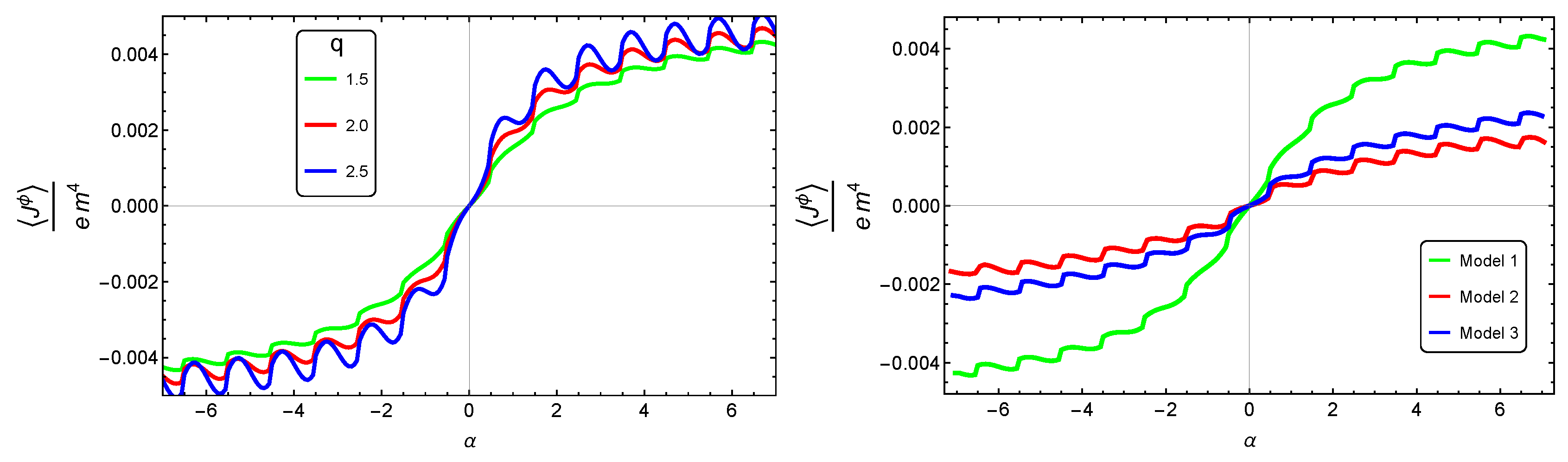
The last important point to be clarified in this paper is about the behavior of the azimuthal core-induced current with the intensity of the magnetic field. In order to do that we present in in Figure 3, the behavior of in units of , as function of for a fixed point. We choose and . The left plot is constructed for the first model of magnetic field and taking with . As we can see, the intensities increase with , however presenting an oscillatory behavior. Moreover, this plot also reinforce the fact that the intensity of the current increases with q. In the right plot all the configurations of magnetic fields are considered. In the latter the parameter q has been fixed equal to . For both plots, we assume that varies in the interval . By them we can infer that the intensity of the core-induced azimuthal current, , increases with , however presenting an oscillatory behavior.
4. Conclusions
In this paper we have investigated the vacuum expectation of the azimuthal fermionic current in a locally flat cosmic string spacetime, admitting the presence of a magnetic field confined inside to a tube of finite radius a. Three distinct configurations of have taken into account. They are: (i) a magnetic field concentrated on a surface of the tube; (ii) a magnetic field presenting a radial dependence; and (iii) an homogeneous magnetic field. In fact, we have concentrated ourselves on the current in the region outside the tube, i.e., in the region with . So, we had to construct the set of normalized solutions of the Dirac equation in the region outside the core in a general formalism, that could be applied to each of the three configurations of magnetic field. Because in general, the analysis of vacuum induced current takes into account only the presence of a magnetic flux running along a line, this present analysis provides some improvements and may shed light in the analysis of induced current in a more realistic model. In fact, the results found here were obtained for fixed configurations of magnetic fields. The complete treatment should take into the equations for fermionic and gauge fields simultaneously. In particular, the result found for the induced current can be used as source of a semiclassical Maxwell’s equations. We understand that our result is a part of a more complete project that may be developed in near future.
By using the mode-sum formula, we have shown that the azimuthal induced current can be written as the sum of two contributions. The first one corresponds to the idealized cosmic string having a magnetic flux running along its core, given by (53), being this one a periodic function of the total flux with the period equal to quantum flux, . The second contribution named core-induced, given by (58), besides to depend on the total magnetic field takes into account a specific configuration for the magnetic field.
The first analysis presented in this paper is related with the behavior of the azimuthal core-induced current in some limits regions. In this sense we have shown that for a massive field, , decays, for as (see (60)). Because the corresponding zero-thickness azimuthal current decays as , the latter dominates the total azimuthal current. In the case of massless field, the core-induced current, (68), decays as , being . Comparing this result with the corresponding one for the zero-thickness azimuthal current which decays with , we conclude that for large distance the total azimuthal current is dominated by the zero-thickness contribution. Finally for point near the tube core, the core-induced current diverges with , as shown by (72). So this contribution is dominant in this region.
Because some informations about the azimuthal core-induced current are not explicitly provided in the analytical analysis, in the last part of our paper we have presented some numerical evaluations of this current, exhibiting its behavior as function of several physical quantities relevant in our analysis. In Figure 1 we have two panels displaying the dependence of with . In the left panel an expected result is presented: The current changes its sign when we change the direction of the magnetic field. In the right panel, it is exhibited the behavior of the current for the three configurations of magnetic field. It is shown that the intensity of the current induced by the first model is the largest one. By these panels we can see that near the core the intensity of the currents become very large, and decay very fast for for massive fields. In Figure 2, we exhibit the behavior of current density for the first model as function of , for fixed value of and different values of q. By this plot we can infer that the intensity of the current increasing with q. Our final numerical analysis is exhibited in Figure 3. There we have displayed how the intensity of depends on for a fixed point. In the left plot we have considered only the first model and varying q. This plot reinforces the fact that the intensity of the current increases with q. The right plot exhibits the behavior of the core-induced current, for the three models, for fixed value of q. Also this plot reinforce that the first model provides the current with biggest intensity. As additional information, we can infer that the intensity of the current increases with the magnetic flux through the parameter , however presenting an oscillatory behavior.
Acknowledgments
Mikael Souto Maior de Sousa thanks Coordenação de Aperfeiçoamento de Pessoal de Nível Superior (CAPES) for financial support. Eugênio Ramos Bezerra de Mello thanks Conselho Nacional de Desenvolvimento Científico e Tecnológico (CNPq), Process No. 313137/2014-5, for partial financial support.
Author Contributions
Eugênio Ramos Bezerra de Mello, Rubens Freire Ribeiro and Mikael Souto Maior de Sousa participated in several steps of this work equally.
Conflicts of Interest
The authors declare no conflict of interest.
Abbreviations
The following abbreviations are used in this manuscript:
| VEV | Vacuum Expectation Value |
| NO | Nielsen and Olesen |
References
- Abrikosov, A.A. On the Magnetic Properties of Superconductors of the Second Group. Zh. Eksp. Teor. Fiz. 1957, 32, 1442–1445. [Google Scholar]
- Nielsen, N.B.; Olesen, P. Vortex-line models for dual strings. Nucl. Phys. B 1973, 61, 45–61. [Google Scholar] [CrossRef]
- Garfinkle, D. General relativistic strings. Phys. Rev. D 1985, 31, 1323–1329. [Google Scholar] [CrossRef]
- Laguna-Castillo, P.; Matzner, R.A. Discontinuity cylinder model of gravitating U(1) cosmic strings. Phys. Rev. D 1987, 35, 2933–2939. [Google Scholar] [CrossRef]
- Bezerra de Mello, E.R.; Bezerra, V.B.; Saharian, A.A.; Tarloyan, A.S. Vacuum polarization induced by a cylindrical boundary in the cosmic string spacetime. Phys. Rev. D 2006, 74, 025017. [Google Scholar] [CrossRef]
- Dowker, J.S. Vacuum averages for arbitrary spin around a cosmic string. Phys. Rev. D 1987, 36, 3742–3746. [Google Scholar] [CrossRef]
- Guimarães, M.E.X.; Linet, B. Scalar Green’s functions in an Euclidean space with a conical-type line singularity. Commun. Math. Phys. 1994, 165, 297–310. [Google Scholar] [CrossRef]
- Guimarães, M.E.X. Vacuum polarization at finite temperature around a magnetic flux cosmic string. Class. Quantum Gravity 1995, 12, 1705. [Google Scholar] [CrossRef]
- Linet, B. Euclidean thermal spinor Green’s function in the spacetime of a straight cosmic string. Class. Quantum Gravity 1996, 13, 97. [Google Scholar] [CrossRef]
- Spinelly, J.; Bezerra de Mello, E.R. Spinor Green function in higher-dimensional cosmic string space-time in the presence of magnetic flux. J. High Energy Phys. 2008, 2008, 005. [Google Scholar] [CrossRef]
- Sitenko, Y.A.; Vlasii, N.D. Induced vacuum energy-momentum tensor in the background of a cosmic string. Class. Quantum Gravity 2012, 29, 095002. [Google Scholar] [CrossRef]
- Sriramkumar, L. Fluctuations in the current and energy densities around a magnetic-flux-carrying cosmic string. Class. Quantum Gravity 2001, 18, 1015–1025. [Google Scholar] [CrossRef]
- Sitenko, Y.A.; Vlasii, N.D. Induced vacuum current and magnetic field in the background of a cosmic string. Class. Quantum Gravity 2009, 26, 195009. [Google Scholar] [CrossRef]
- Bezerra de Mello, E.R. Induced fermionic current densities by magnetic flux in higher dimensional cosmic string spacetime. Class. Quantum Gravity 2010, 27, 095017. [Google Scholar] [CrossRef]
- Bezerra de Mello, E.R.; Saharian, A.A. Fermionic current induced by magnetic flux in compactified cosmic string spacetime. Eur. Phys. J. C 2013, 73, 2532. [Google Scholar] [CrossRef]
- Bragança, E.A.F.; Santana Mota, H.F.; Bezerra de Mello, E.R. Induced vacuum bosonic current by magnetic flux in a higher dimensional compactified cosmic string spacetime. Int. J. Mod. Phys. D 2015, 24, 1550055. [Google Scholar] [CrossRef]
- Spinelly, J.; Bezerra de Mello, E.R. Vacuum polarization of a charged massless scalar field on cosmic string spacetime in the presence of a magnetic field. Class. Quantum Gravity 2003, 20, 873–887. [Google Scholar] [CrossRef]
- Spinelly, J.; Bezerra de Mello, E.R. Vacuum polarizations of a charged massless fermionic field by a magnetic flux in the cosmic string spacetime. Int. J. Mod. Phys. D 2004, 13, 607–624. [Google Scholar] [CrossRef]
- Spinelly, J.; Bezerra de Mello, E.R. Vacuum polarization by a magnetic flux in a cosmic string background. Nucl. Phys. B Proc. Suppl. 2004, 127, 77–83. [Google Scholar] [CrossRef]
- Bezerra de Mello, E.R.; Bezerra, V.B.; Saharian, A.A.; Harutyunyan, H.H. Vacuum currents induced by a magnetic flux around a cosmic string with finite core. Phys. Rev. D 2015, 91, 064034. [Google Scholar] [CrossRef]
- Bordag, M.; Khusnutdinov, N. A remark on bound states in conical spacetime. Class. Quantum Gravity 1996, 13, L41–L45. [Google Scholar] [CrossRef]
- Gradshteyn, I.S.; Ryzhik, I.M. Table of Integrals, Series and Products; Academic Press: New York, NY, USA, 1980; pp. 909–1475. [Google Scholar]
- De Mello, E.R.B.; Bezerra, V.B.; Saharian, A.A.; Bardeghyan, V.M. Fermionic current densities induced by magnetic flux in a conical space with a circular boundary. Phys. Rev. D 2010, 82, 085033. [Google Scholar] [CrossRef]
- De Sousa, M.S.M.; Ribeiro, R.F.; Bezerra de Mello, E.R. Induced fermionic current by a magnetic tube in the cosmic string spacetime. Phys. Rev. D 2016, 93, 043545. [Google Scholar] [CrossRef]
- Maior de Sousa, M.S.; Ribeiro, R.F.; Bezerra de Mello, E.R. Fermionic vacuum polarization by an Abelian magnetic tube in the cosmic string spacetime. Phys. Rev. D 2017, 95, 045005. [Google Scholar] [CrossRef]
- Abramowitz, M.; Stegun, I.A. Handbook of Mathematical Functions; National Bureau of Standards: Washington, DC, USA, 1964; pp. 503–510. [Google Scholar]
Figure 1.
In the above picture the core-induced fermionic current are displayed in units of , as function of assuming and . In the left panel two distinct values of magnetic field are considered: and . The right panel exhibits the behavior of the currents induced by the three configurations of magnetic fields considering .

Figure 2.
This plot presents the behavior of the azimuthal core-induced current as function of , considering three distinct values for q exhibit in the plot.
Figure 2.
This plot presents the behavior of the azimuthal core-induced current as function of , considering three distinct values for q exhibit in the plot.

Figure 3.
The core-induced azimuthal current density is exhibited as function of varying in the interval for a fixed point outside the core. Specifically we have chosen and . The left plot display the current considering only the first model and different values of q; as to the right plot we display the current induced by the three configurations of magnetic fields considering .

© 2018 by the authors. Licensee MDPI, Basel, Switzerland. This article is an open access article distributed under the terms and conditions of the Creative Commons Attribution (CC BY) license (http://creativecommons.org/licenses/by/4.0/).
Share and Cite
MDPI and ACS Style
Maior de Sousa, M.S.; Freire Ribeiro, R.; Bezerra de Mello, E.R. Azimuthal Fermionic Current in the Cosmic String Spacetime Induced by a Magnetic Tube. Particles 2018, 1, 82-96. https://doi.org/10.3390/particles1010006
AMA Style
Maior de Sousa MS, Freire Ribeiro R, Bezerra de Mello ER. Azimuthal Fermionic Current in the Cosmic String Spacetime Induced by a Magnetic Tube. Particles. 2018; 1(1):82-96. https://doi.org/10.3390/particles1010006
Chicago/Turabian StyleMaior de Sousa, Mikael Souto, Rubens Freire Ribeiro, and Eugênio Ramos Bezerra de Mello. 2018. "Azimuthal Fermionic Current in the Cosmic String Spacetime Induced by a Magnetic Tube" Particles 1, no. 1: 82-96. https://doi.org/10.3390/particles1010006