Bulk Viscosity of Hot Quark Plasma from Non-Equilibrium Statistical Operator


1
Institute for Theoretical Physics, Goethe University, Max-von-Laue-Straße, 1, 60438 Frankfurt am Main, Germany
2
Frankfurt Institute for Advanced Studies, Ruth-Moufang-Straße, 1, 60438 Frankfurt am Main, Germany
*
Author to whom correspondence should be addressed.
Particles 2018, 1(1), 212-229; https://doi.org/10.3390/particles1010016
Submission received: 18 June 2018
/
Revised: 23 July 2018
/
Accepted: 13 August 2018
/
Published: 20 August 2018
(This article belongs to the Special Issue Selected Papers from “The Modern Physics of Compact Stars and Relativistic Gravity 2017”)
Abstract
:We provide a discussion of the bulk viscosity of two-flavor quark plasma, described by the Nambu–Jona-Lasinio model, within the framework of Kubo-Zubarev formalism. This discussion, which is complementary to our earlier study, contains a new, detailed derivation of the bulk viscosity in the case of multiple conserved charges. We also provide some numerical details of the computation of the bulk viscosity close to the Mott transition line, where the dissipation is dominated by decays of mesons into quarks and their inverse processes. We close with a summary of our current understanding of this quantity, which stresses the importance of loop resummation for obtaining the qualitatively correct result near the Mott line.
1. Introduction
Transport coefficients of hot and dense quark plasma are key inputs in the hydrodynamical description of the heavy-ion experiments at Relativistic Heavy Ion Collider (RHIC) and Large Hadron Collider (LHC). The matter created in these experiments exhibits a very small ratio of the shear viscosity to the entropy density, which is close to the lower bound placed by the uncertainty principle [1] and conjectured on the basis of AdS/CFT duality [2].
The bulk viscosity describes the dissipation in cases where pressure falls out of its equilibrium value on uniform expansion or contraction of fluid. It vanishes in several cases, e.g., for an ultrarelativistic or nonrelativistic gas interacting weakly with local forces via binary collisions, as well as in strongly coupled systems with conformal symmetry. Because at high energies QCD is almost conformally symmetric, the bulk viscosity of quark-gluon plasma is small in the perturbative regime [3,4,5,6]. At low energies, the conformal symmetry is broken by the quark mass and/or by dimensionful regularization of the ultraviolet divergences, in which case the bulk viscous effects can become important. Large values of bulk viscosity were found, in particular, close to the chiral phase transition line [7,8]. Computations of the QCD bulk viscosity in the strongly coupled regime where carried out using various methods including lattice simulations [5,9,10], quasiparticle Boltzmann transport [11,12,13,14,15] and the Kubo formalism [16,17,18].
The focus of this contribution, which is complementary to our earlier study [16], is the bulk viscosity of quark matter in the non-perturbative regime as it is realized close to the chiral phase transition line. The case of bulk viscosity is special because it requires a resummation of an infinite series of loop diagrams, whereas the remaining coefficient (shear viscosity, thermal and electrical conductivities) are given by the one-loop result only, see Ref. [19]. Specifically, our aim here is to provide details of the computation of this quantity which complement our earlier publication [16]. First, we provide a formal derivation of the bulk viscosity coefficient from the Zubarev formalism of non-equilibrium statistical operator (NESO) [20,21] in a general setting of relativistic quantum field theory assuming a system with multiple conserved charges. We then go on to discuss the details of diagrammatic evaluation of the bulk viscosity within the Nambu–Jona-Lasinio (NJL) model, which is an effective field theory of QCD that captures its chiral symmetry breaking feature. The main mechanism of dissipation within this model is provided by the mesonic fluctuations close to the critical line of chiral phase transition.
Another important ingredient of the diagrammatic evaluation of the two-point correlation function determining the bulk viscosity is the expansion [22]. Several recent computations of bulk viscosity, which were based on a Kubo formula and the NJL model, evaluated the relevant correlation function at the one-loop level [17,18]. However, our recent analysis [16] indicates, that the one-loop approximation is not consistent with the power counting scheme and a resummation of infinite series of loop diagrams is required to obtain the leading-order approximation to the bulk viscosity. Below, we provide some numerical details of this computation.
This work is organized as follows. In Section 2 we review Zubarev’s method of the NESO and derive a Kubo-type formula for the bulk viscosity. Section 3 is devoted to the application of the general formalism to the case of two-flavor quark matter described by the NJL model. Our numerical results for the bulk viscosity are collected in Section 4. Section 5 provides a short summary. The computation of a Matsubara sum, which is used in the derivation of the Kubo formula, is relegated to Appendix A. We use the natural (Gaussian) units with , and the metric signature .
2. Bulk Viscosity Formula from the Non-Equilibrium Statistical Operator
The coefficient of the bulk viscosity was computed within the NESO method for the case of a system without conserved charges in the seminal paper by Hosoya et al. [23]. Our purpose here is to extend that derivation to the case of systems with multiple conserved charges.
Hydrodynamics of relativistic quantum fluids is described by the energy-momentum tensor and currents of conserved charges . We consider the general case of multiple conserved charge flavors (e.g., baryonic, electric, etc.) which are labeled by the index a. In this case, these conservation laws take the form
For systems in the hydrodynamic regime, one can introduce local thermodynamic variables, such as temperature , chemical potentials and fluid 4-velocity as smooth functions of the space-time coordinates . Below we will specify the (matching) conditions which are necessary to identify these quantities. Our next step is to define a NESO as
with operators defined as
where the covariant quantities (c-numbers) are defined as
Note that the limit in Equation (4) should be taken only after the thermodynamic limit. The proper order of taking the thermodynamic and limits guarantees that the NESO in Equation (2) satisfies the Liouville equation with an infinitesimal source term, which breaks the time-reversibility of that equation and chooses its retarded solution for positive values of [20,21,23]. Equations (2)–(6) generalize the analogous expressions of Refs. [23,24] to the case of a system with multiple conserved charges.
The first term in the exponent in Equation (2) corresponds to the local equilibrium part of the statistical operator, defined as
The second term in the exponent of Equation (2) is the non-equilibrium part of the statistical operator, which can be interpreted as a thermodynamic “force”. For small deviations from equilibrium, it can be treated as a small perturbation. Expanding the NESO around the local equilibrium distribution and keeping linear in the operator terms we find
The statistical average of any operator can be written now as
where is the local equilibrium average and a two-point correlation function has been defined as [23,24]
The final point of our general discussion of the NESO method is the procedure by which the quantities and are matched with the relevant thermodynamic variables in an arbitrary non-equilibrium state. This can be achieved by the following matching conditions [20,21,24]
where the operators of the energy and charge densities are defined as and . In these expressions, the fluid 4-velocity , which is normalized to unity , should be “tied” to a physical current. This could be either the energy flow, which specifies the Landau-Lifshitz frame [25] or the charge flow, which specifies the Eckart frame [26]. In the Landau frame , whereas in the Eckart frame . The conditions (11) define the temperature and the chemical potentials of components as non-local functionals of and [27]. However, the hydrodynamic description requires thermodynamic parameters as local functions of the energy and charge densities. In practice, this difficulty is circumvented by dividing the fluid into elements which are in local statistical equilibrium and each of which is independent of the other [28]. In practice, the local equilibrium values and in Equation (11) are then evaluated assuming formally constant values of and , which are identified by matching and to the real values of these quantities and at any given point x. In this way one can construct a fictitious local equilibrium state, characterized by the thermodynamic parameters and , such that it reproduces the local values of the energy and charge densities at every point of the space and time.
2.1. Decomposition into Different Dissipative Processes
To identify the different dissipative processes, we now exploit the common decompositions of the energy-momentum tensor and the charge currents into the ideal and dissipative parts
where is the operator of pressure; is the projection operator onto the 3-space orthogonal to and has the properties
The dissipative quantities , and are the operators of the shear stress tensor, energy diffusion flux and charge diffusion fluxes, respectively, and they satisfy the following conditions
The operators on the right-hand sides of Equations (12) and (13) can be obtained via the projections of and
which in the local rest frame [] read
In Equation (17) we introduced a fourth-rank traceless projector orthogonal to
The hydrodynamic quantities , and are obtained as the statistical averages of the corresponding operators over the NESO according to Equations (9) and (10). In local equilibrium the averages of the dissipative operators vanish:
To compute the non-equilibrium averages of these operators it is convenient to write the operator given by Equation (5) as a sum of contributions of different dissipative processes according to Equations (12) and (13). Similar decompositions were performed in Refs. [23,24]. Recalling the properties (14) and (15) we obtain
where we introduced the covariant time-derivative , the covariant spatial derivative , the fluid expansion rate and the velocity stress tensor via . As a first approximation, we can eliminate the terms , and using the equations of ideal hydrodynamics
where is the equilibrium pressure fixed by an equation of state, and is the enthalpy density. Choosing and as independent thermodynamic variables and using the first two equations in (23) we can write
2.2. Kubo Formula for the Bulk Viscosity
By definition, bulk viscous pressure measures the deviation of the thermodynamic pressure from its equilibrium value, which results from the expansion or compression of the fluid. Therefore, it might appear at a first glance that the bulk viscous pressure should be identified as . However, it is easy to see that such a definition would be erroneous. To understand the problem, we go back to the matching conditions (11), which define the local equilibrium state. As explained above, these conditions are satisfied only if the local equilibrium distribution function is evaluated formally assuming uniform background values of the thermodynamic parameters, i.e., as if these were constant in space and time with the given values and . Because the local equilibrium distribution (7) is actually a functional of non-uniform thermodynamic parameters, the average values and in the full computation are shifted from the actual values of and by additional gradient terms and , which were neglected in Equation (11). These shifts bring, in their turn, an additional shift in the equilibrium part of the pressure , which should not be included in the bulk viscous pressure [4,29,30]. Thus, the bulk viscous pressure should be defined as the difference between the actual non-equilibrium pressure and the equilibrium pressure , which is not equal to :
where we kept only the linear terms. Then, the bulk viscous pressure is given by
where we used the definition of given by Equation (31). From Equations (9), (22) and (30) we then obtain
where we dropped the correlators between operators of different rank, because they vanish in isotropic medium according to Curie’s theorem [31]. Introducing the bulk viscosity as
we rewrite Equation (34) as
The correlator (35) can be evaluated using uniform background values of thermodynamic parameters, i.e., as if the system is in global thermal equilibrium. Finally, the bulk viscosity can be cast in the form of a Kubo formula [23,24]
where the two-point retarded equilibrium Green’s function in the zero-wavenumber limit is given by
where the square brackets denote a commutator.
3. Bulk Viscosity within the Two-Flavor NJL Model
In this section, we illustrate the computation of the bulk viscosity following Ref. [16]; in doing so we will provide some numerical details not exposed earlier. The Lagrangian of the two-flavor NJL model contains scalar-isoscalar and pseudoscalar-isovector channels of interactions among quarks and is given by
where is the Dirac field for u and d quarks, MeV is the current-quark mass, GeV is the effective coupling and is the vector of Pauli matrices in the space of isospin. The NJL model is regularized with a three-momentum cut-off GeV. Assuming isospin-symmetry, the only conserved current is the net particle current given by
The energy-momentum tensor reads
The relevant operator which enters the Kubo formula (37) with the correlator given by Equation (38) in the local rest frame reads (see Equations (18) and (31))
Inserting Equation (42) back into Equation (38) and using the symmetry relations , etc., we obtain
where we omitted the arguments of the operators. Substituting here the explicit expressions for and and switching to the imaginary-time (Matsubara) formalism via the substitutions , , we obtain
with two-point correlation functions defined as
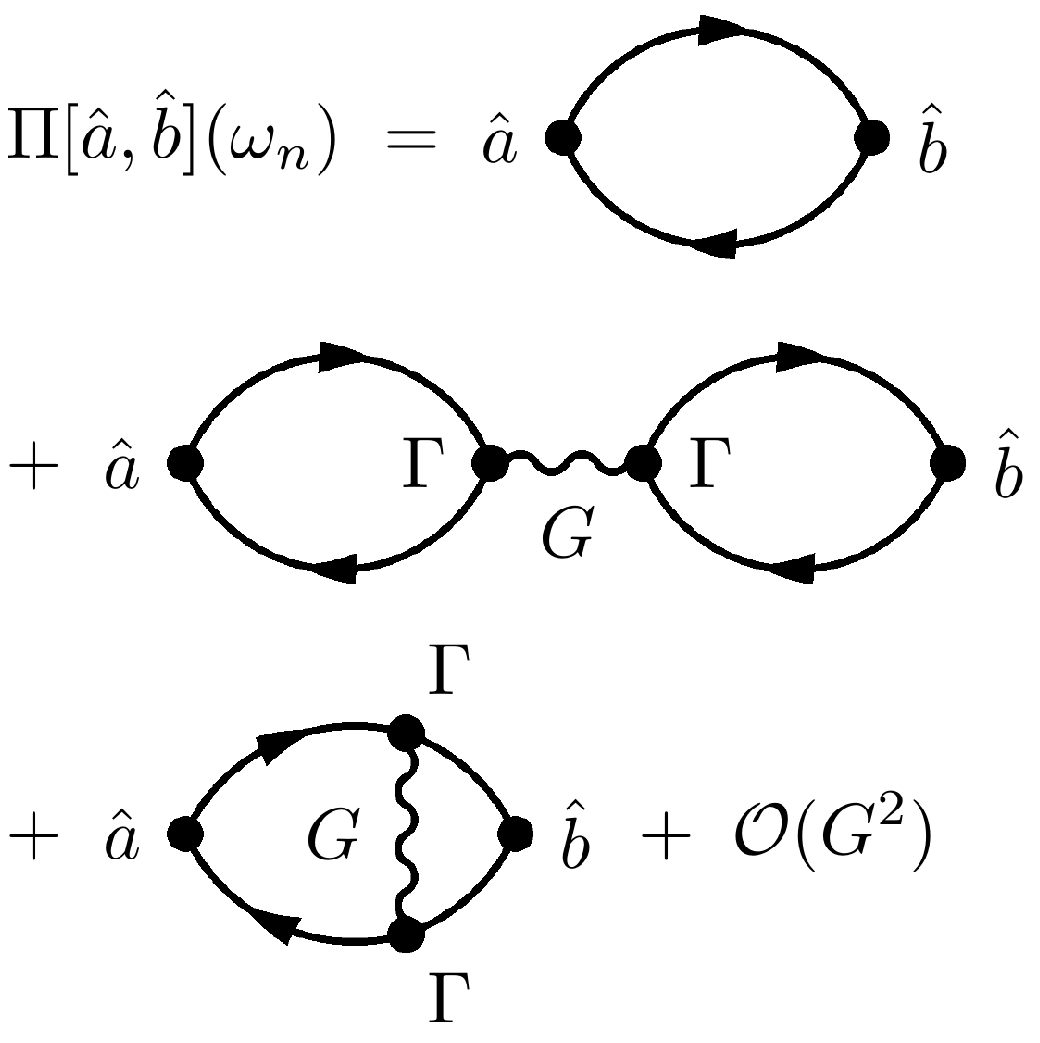
where , are the bosonic Matsubara frequencies; is the imaginary time-ordering operator; , and and are either constants or -matrices contracted with partial derivatives. (Note that the correlators which arise from the interaction part of Equation (39) vanish for because of the energy conservation, see Ref. [16] for details). Figure 1 illustrates diagrammatically the series of the loop diagrams which contribute to the correlation function given by Equation (45).
Resummation of the Feynman Diagrams
The class of leading-order diagrams which contributes to the correlation function (45) is identified according to the power-counting scheme. In this scheme each diagram is selected according to its power with respect to the color number , which is determined by the following rules [22]: (a) each quark loop contributes a factor of , which arises from the trace over the color space; (b) each coupling G contributes a factor of . It is easy to see that the leading-order diagrams in the correlation function (45) are of the order of and involve loop diagrams without vertex corrections, i.e., those of the type shown in the first and the second lines in Figure 1. Indeed, the factor associated with each additional loop is compensated by the factor from an interaction insertion. Therefore, we conclude that we need to resume an infinite chain of loop diagrams without vertex corrections. To carry out the resummation, define the single-loop diagram in the momentum space as
where is the full (i.e., dressed) quark propagator defined in the imaginary time, and the summation is over the fermionic Matsubara frequencies , where is the quark chemical potential. The traces should be taken in Dirac, color, and flavor spaces. The resummation then leads to
where (the correlators with the pseudoscalar vertex vanish because the relevant traces vanish in the Dirac space). The frequency arguments in Equation (47) were omitted for the sake of brevity. The effective coupling in Equation (47) is related to the bare coupling G via
The diagrams involving vertex corrections, such as the one shown in the third line of Figure 1, are of higher order in the power-counting scheme. Thus, the computation of the leading-order contribution to the bulk viscosity reduces to the calculation of the series of loop diagrams defined by Equation (47), which in turn requires the evaluation of the single-loop diagram given by Equation (46). To carry out the sum over the Matsubara frequencies in Equation (46) one needs the frequency dependence of the operators and which arises when [see Equation (44)]. Indeed, in the frequency space, such dependence translates as . For such cases, we separate the -dependence by formally factorizing the frequency dependence into a function , i.e., we write , where and do not depend on . After summation over the Matsubara frequencies and subsequent analytical continuation (i.e., ) we obtain (see Appendix A for details)
where with being the Fermi distribution for quarks. Finally, we separate the real and imaginary parts in Equation (49) by exploiting the Dirac identity
From Equations (49) and (50) we find
and
Using Equation (52) we can compute the imaginary part of Equation (47)
where
To compute the traces in Equations (49) and (51) one needs to exploit the Dirac decomposition of the spectral function
where m is the quark mass. The coefficients , and can be expressed in terms of the relevant components of the quark self-energy according to the relations [19,32,33]
where , , , and
From now on we will neglect the irrelevant real parts of the self-energy, which lead to momentum-dependent corrections to the constituent quark mass in next-to-leading order and will keep only the imaginary parts which were computed in Refs. [19,32,33]. The three components of the quark self-energy are identified via
With this input, we can now calculate the relevant correlators entering Equation (44). Computing the traces and performing the angular integrations in Equations (49) and (51), we find, e.g.,
where ; and are the color and flavor numbers, respectively. The remaining correlation functions can be computed in analogy to Equations (64) and (65); the explicit expressions are given in Ref. [16].
Inserting the relevant correlators in Equations (37), (44), (53)–(58), we can write the bulk viscosity as
where each of the three terms arises from the corresponding terms in Equation (53). The first (single-loop) term is given by
where and The multiloop contributions are given by
where the effective coupling is given by
with the polarization loop
and
Here the functions are obtained from defined above by substitution . Equations (66)–(73) express the bulk viscosity of quark plasma in terms of the components of its spectral function.
It is remarkable that the multiloop contributions to the bulk viscosity vanish trivially in the chirally symmetric case, where . Indeed, for massless quarks and temperatures , where is the critical temperature of the chiral phase transition, we find and in Equation (70). As a result, we have and according to Equations (68) and (66).
4. Numerical Results
We use the Lorentz components of the quark spectral function, obtained previously in Refs. [19,32,33], to evaluate numerically the bulk viscosity. We concentrate on the region of the phase diagram which is located above the Mott transition temperature , which is defined as the threshold temperature at any given chemical potential above which the meson decay into two on-mass-shell quarks is kinematically allowed. It is identical to the chiral phase transition temperature in the chiral limit .
To gain insight into the numerical results for the bulk viscosity, it is useful first to analyze the integrands of Equations (67) and (70)–(73). The integrands of , and are shown in Figure 2. Each of these integrands develops a peak structure at , whereby the height of the peak rapidly increases with . The momentum integrals are increasing functions of as long as , and decreasing for larger energies (because of the momentum cut-off , see Figure 2).
Note that for the integrands are even functions of , which reflects the quark-antiquark symmetry. The factor breaks this symmetry for non-vanishing chemical potentials by increasing the contribution of quarks. Thus, we see that the dominant contribution to the bulk viscosity comes from the modes with , whereby the quark contribution dominates the antiquark contribution at non-zero .
Now we turn to the three-dimensional integrals and given by Equations (70) and (73). Their integrands are strongly peaked at , and have two smaller maxima located at and in the cases where , see Figure 3. As a result, the momentum integrals of these expressions obtain the main contribution form energies . We also observe that the height of each peak increases with for and sharply drops beyond the cut-off. The peak structures seen above reflect the quasiparticle-like nature of the excitations, which however have non-zero width because of the meson decay and recombination processes included in our consideration.
Figure 4 illustrates the temperature and chemical potential dependence of the integrals , , and the renormalized coupling [given by Equation (58)]. The behavior of is similar to and is not shown. Quantitatively, the three- and two-dimensional integrals and , respectively, show the same behavior, reflecting the importance of the meson decay processes close to the Mott line. The renormalized coupling attains its maximum close to the Mott line, where it exceeds the bare coupling constant roughly by an order of magnitude. Because of this behavior of , the multiloop contributions to the bulk viscosity given by Equation (68) are expected to be important close to the Mott temperature.
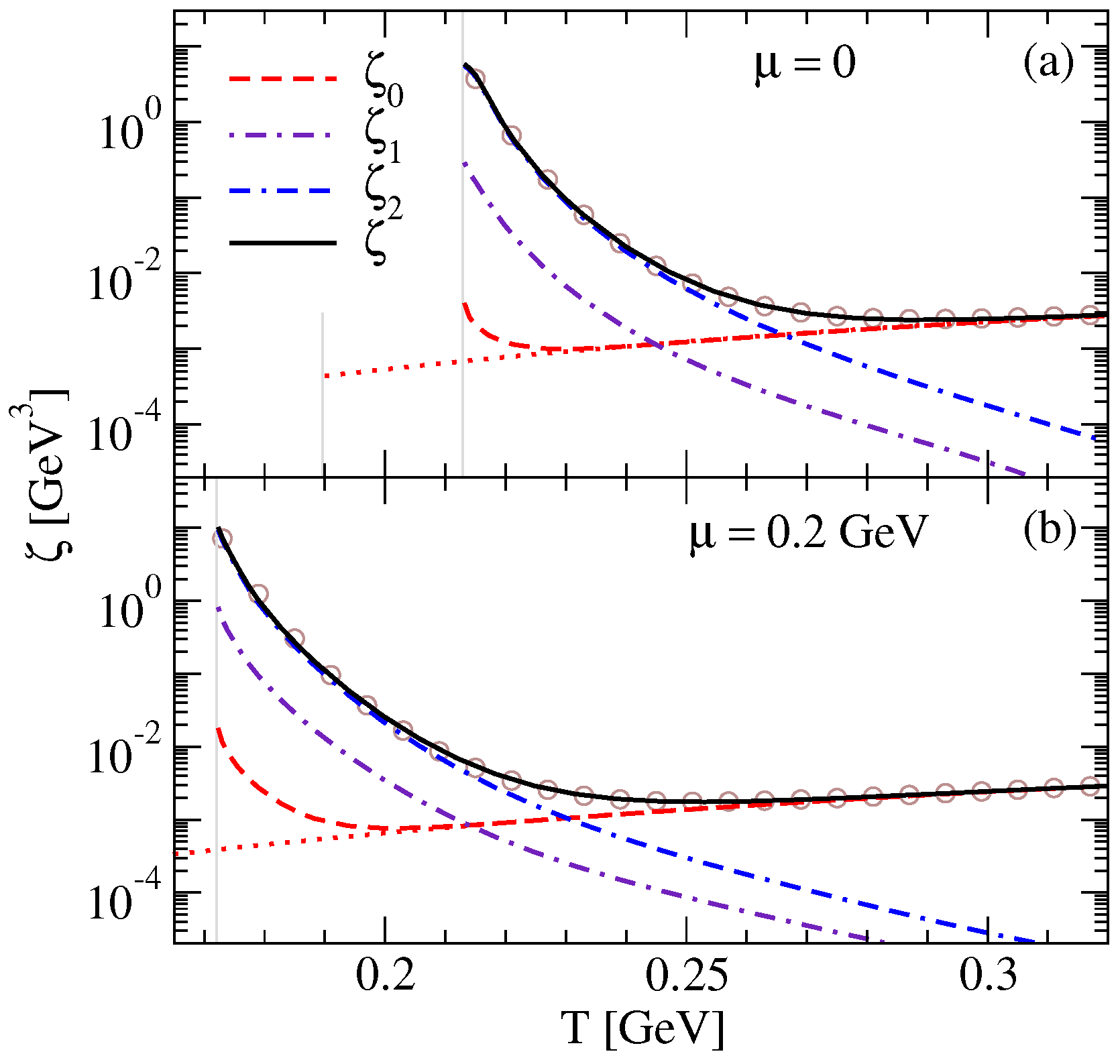
The results for the bulk viscosity are shown in Figure 5. The multiloop contributions and dominate over the one-loop contribution in the regime close to the Mott transition line, where all three components rapidly decrease with the temperature and density. At high enough temperatures, the one-loop contribution scales as and dominates over the multiloop contributions. The net bulk viscosity which is the sum of the one-loop and multiloop contributions then exhibits a shallow minimum as a function of temperature. From the analysis above, we thus conclude that the single-loop approximation is justified only at sufficiently high temperatures where multiloop diagrams are suppressed.
We now comment briefly on the case where the chiral symmetry is intact, i.e., . In this case, the multiloop contributions vanish automatically, as explained in Section 3. The bulk viscosity is then given by the single-loop contribution taken in the limit , which is shown in Figure 5 by the dotted lines for zero and finite chemical potentials. Contrary to the case where , here is smooth at the Mott temperature and increases with the temperature in the whole temperature-density range. We thus conclude that the explicit chiral symmetry breaking is essential for the correct description of the bulk viscosity in the low-temperature region of the phase diagram, especially in the region close to the chiral phase transition line.
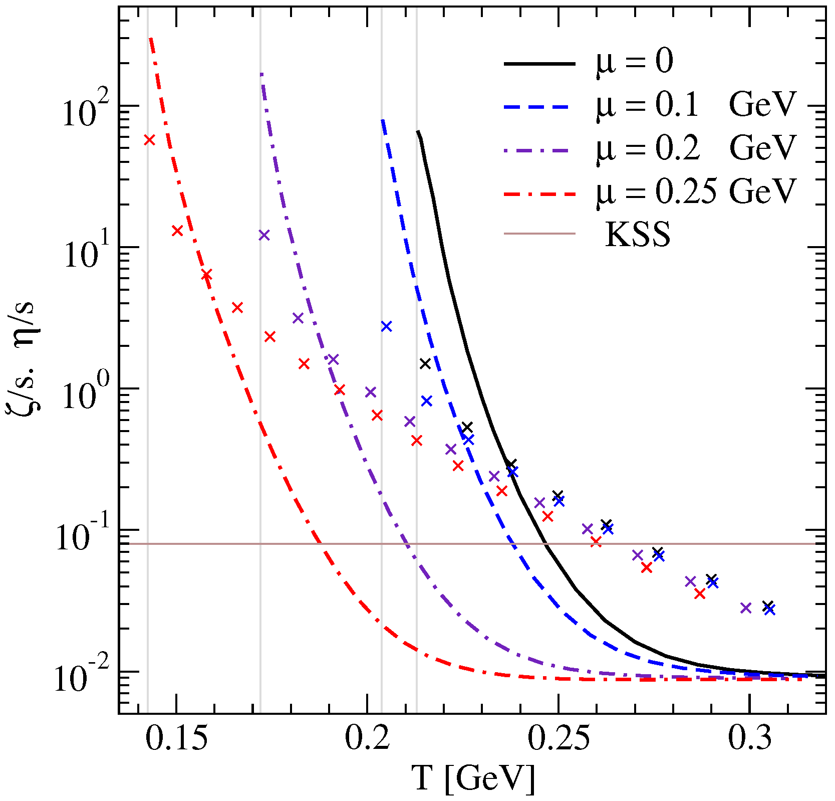
For completeness, we also compare our results with the shear viscosity , which was computed previously in Ref. [19] (see also Refs. [32,33]) by employing the same formalism and approximations. Figure 6 shows the dependence of the ratios and , where s is the entropy density, on the temperature for several values of the chemical potential [16,19]. For comparison, we also show the AdS/CFT lower bound on the ratio [2]. We see that both ratios decrease rapidly with the temperature, but the slope of this decrease is larger in the case of the bulk viscosity in the region which is close to the Mott transition line. In this regime, the bulk viscosity exceeds the shear viscosity by factors . Thus, in the low-temperature regime close to the Mott transition line the bulk viscosity is the dominant source of dissipation. It is worth stressing that had we kept only the one-loop contribution to the bulk viscosity, it would have been negligible compared to the shear viscosity. As drops much faster than with the temperature, the shear viscosity is the dominant dissipation channel at high temperatures.
Our numerical results can be fitted using the formula
where , and GeV is the value of the chemical potential at which the Mott line terminates. The coefficients depend only on the chemical potential and are given by
The relative error of the fit formula (74) is for chemical potentials GeV. The bulk viscosity according to our fit formula is shown in Figure 5 by empty circles. The fit formula above should be complemented by a fit to the Mott temperature as a function of the chemical potential, which is given by the formula
where GeV, and . The relative accuracy of the formula (79) is for chemical potentials GeV.
5. Conclusions
In this contribution, we provided a general derivation of the Kubo formula for the bulk viscosity from Zubarev’s formalism of NESO generalized to systems with multiple conserved charges. The method was then illustrated on the example of computation of the bulk viscosity of quark matter in the framework of the two-flavor NJL model. The previous discussion of Ref. [16] has been supplemented by further details.
The key finding of our work is that at low temperatures and close to the Mott transition line the overall multiloop contribution to the bulk viscosity is larger than the one-loop contribution. This is in contrast to the results found for the shear viscosity and the thermal and electrical conductivities, for which the single-loop approximation gives the leading-order result [19]. We have shown that the bulk viscosity decreases with the temperature and the chemical potential in this regime, attains a minimum and then increases again at higher temperatures where the one-loop contribution becomes dominant.
Phenomenologically interesting is the fact that the bulk viscosity provides the main source of dissipation of stresses close to the Mott line as it exceeds the shear viscosity in this regime by factors of . The bulk viscosity drops faster than the shear viscosity as the temperature increases and it becomes negligible above a certain value of the temperature. Finally, we observed that in the chiral symmetric case, where the quark masses vanish above the (critical) Mott temperature, the picture is different. In this case, the multiloop contributions to the bulk viscosity vanish, and consequently the bulk viscosity becomes negligible compared to the shear viscosity in the entire temperature-density plane.
Author Contributions
Conceptualization, A.H., A.S.; Methodology, A.H., A.S.; Investigation, A.H., A.S.; Writing—Original Draft Preparation, A.H., A.S.; Writing—Review & Editing, A.H., A.S.; Funding Acquisition, A.S.
Funding
This research was funded by Deutsche Forschungsgemeinschaft, grant number SE 1836/4-1 and by European Cooperation in Science and Technology (Actions MP1304 and CA16214).
Acknowledgments
We are grateful to Xu-Guang Huang and Dirk H. Rischke for discussions. A.H. acknowledges support from the HGS-HIRe graduate program at Goethe University. A.S. was supported by the Deutsche Forschungsgemeinschaft (Grant No. SE 1836/4-1). The support from European COST Actions “NewCompStar” (MP1304) and “PHAROS” (CA16214) and the LOEWE-Program of Helmholtz International Center for FAIR of the state of Hesse (Germany) is gratefully acknowledged.
Conflicts of Interest
The authors declare no conflict of interest.
Appendix A. Matsubara Summations
To perform the Matsubara summation in Equation (46) we express the full quark propagator in terms of the quark spectral function
where the spectral function is defined as
with being the retarded/advanced Green’s functions. According to Equation (A1), has a branch cut on the real axis, therefore a calculation of the residues gives for the integrand of Equation (46)
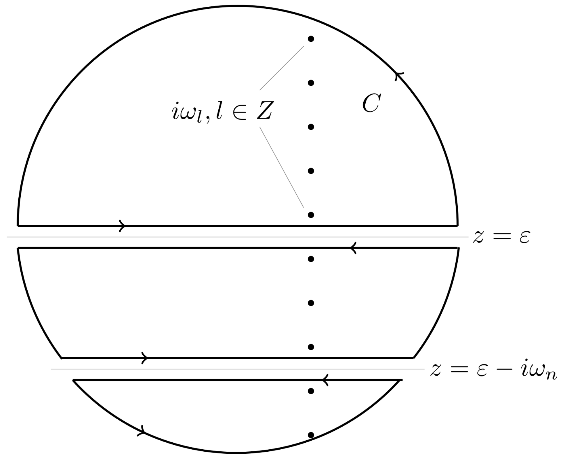
where is the Fermi distribution function, and . The integration contour C is shown in Figure A1, where the circle should be taken infinitely large in order to include all poles of the function . Note that due to the fact that does not coincide with for any n and l, the poles of do not lie on the branch cuts of C.
Figure A1.
The contour of integration in Equation (A3). The dots correspond to the fermionic Matsubara frequencies.
Figure A1.
The contour of integration in Equation (A3). The dots correspond to the fermionic Matsubara frequencies.

We show now that the contribution of the large circle to the integral (A3) vanishes. Because of the sum rule , the quark propagator for large has the scaling . Therefore, for large the integrand in Equation (A3) scales as (recall that ). For the Fermi distribution function we have the asymptotics and . Substituting , , and performing the limit , we can write for the integral along the circle
As seen from Equation (A4), the integral vanishes in the limit if . If , we have , which is purely real and can be dropped since in this case we need only the imaginary parts of functions. As a result, we need to keep only the integrals along the two branch cuts shown in Figure A1. Then, using also Equation (A2), we obtain for Equation (A3)
where we took into account that . Substituting the spectral representation (A1) into Equation (A5), changing the variables in the first term and performing analytical continuation via , we find
Substituting this expression into Equation (46), we obtain Equation (49) of the main text.
References
- Danielewicz, P.; Gyulassy, M. Dissipative phenomena in quark-gluon plasmas. Phys. Rev. D 1985, 31, 53–62. [Google Scholar] [CrossRef] [Green Version]
- Kovtun, P.; Son, D.; Starinets, A. Viscosity in Strongly Interacting Quantum Field Theories from Black Hole Physics. Phys. Rev. Lett. 2005, 94, 111601. [Google Scholar] [CrossRef] [PubMed]
- Hosoya, A.; Kajantie, K. Transport coefficients of QCD matter. Nucl. Phys. B 1985, 250, 666–688. [Google Scholar] [CrossRef]
- Arnold, P.; Doǧan, Ç.; Moore, G.D. Bulk viscosity of high-temperature QCD. Phys. Rev. D 2006, 74, 085021. [Google Scholar] [CrossRef]
- Moore, G.; Saremi, O. Bulk viscosity and spectral functions in QCD. Phys. Rev. D 2008, 9, 015. [Google Scholar] [CrossRef]
- Chen, J.-W.; Liu, Y.-F.; Song, Y.-K.; Wang, Q. Shear and bulk viscosities of a weakly coupled quark gluon plasma with finite chemical potential and temperature: Leading-log results. Phys. Rev. D 2013, 87, 036002. [Google Scholar] [CrossRef]
- Meyer, H. Calculation of the Bulk Viscosity in SU(3) Gluodynamics. Phys. Rev. D 2008, 100, 162001. [Google Scholar] [CrossRef] [PubMed]
- Paech, K.; Pratt, S. Origins of bulk viscosity in relativistic heavy ion collisions. Phys. Rev. C 2006, 74, 014901. [Google Scholar] [CrossRef]
- Karsch, F.; Kharzeev, D.; Tuchin, K. Universal properties of bulk viscosity near the QCD phase transition. Phys. Lett. B 2008, 663, 217–221. [Google Scholar] [CrossRef]
- Aarts, G. Transport and spectral functions in high-temperature QCD. arXiv, 2007; arXiv:0710.0739. [Google Scholar]
- Sasaki, C.; Redlich, K. Transport coefficients near chiral phase transition. Nucl. Phys. A 2010, 832, 62–75. [Google Scholar] [CrossRef] [Green Version]
- Chakraborty, P.; Kapusta, J. Quasiparticle theory of shear and bulk viscosities of hadronic matter. Phys. Rev. C 2011, 83, 014906. [Google Scholar] [CrossRef]
- Chandra, V. Bulk viscosity of anisotropically expanding hot QCD plasma. Phys. Rev. D 2011, 84, 09402. [Google Scholar] [CrossRef]
- Dobado, A.; Llanes-Estrada, F.; Torres-Rincon, J. Bulk viscosity and energy-momentum correlations in high energy hadron collisions. Eur. Phys. J. C 2012, 72, 1873. [Google Scholar] [CrossRef]
- Marty, R.; Bratkovskaya, E.; Cassing, W.; Aichelin, J.; Berrehrah, H. Transport coefficients from the Nambu-Jona-Lasinio model for SU(3)f. Phys. Rev. C 2013, 88, 045204. [Google Scholar] [CrossRef]
- Harutyunyan, A.; Sedrakian, A. Bulk viscosity of two-flavor quark matter from the Kubo formalism. Phys. Rev. D 2017, 96, 034006. [Google Scholar] [CrossRef] [Green Version]
- Xiao, S.-S.; Guo, P.-P.; Zhang, L.; Hou, D.-F. Bulk viscosity of hot dense Quark matter in the PNJL model. Chin. Phys. C 2014, 38, 054101. [Google Scholar] [CrossRef] [Green Version]
- Ghosh, S.; Peixoto, T.; Roy, V.; Serna, F.; Krein, G. Shear and bulk viscosities of quark matter from quark-meson fluctuations in the Nambu-Jona-Lasinio model. Phys. Rev. C 2016, 93, 045205. [Google Scholar] [CrossRef]
- Harutyunyan, A.; Rischke, D.H.; Sedrakian, A. Transport coefficients of two-flavor quark matter from the Kubo formalism. Phys. Rev. D 2017, 95, 114021. [Google Scholar] [CrossRef] [Green Version]
- Zubarev, D. Nonequilibrium Statistical Thermodynamics; Studies in Soviet Science; Consultants Bureau: New York, NY, USA, 1974. [Google Scholar]
- Zubarev, D.; Morozov, V.; Röpke, G. Statistical Mechanics of Nonequilibrium Processes; Akademie Verlag: Berlin, Germany, 1996. [Google Scholar]
- Quack, E.; Klevansky, S. Effective 1/Nc expansion in the Nambu-Jona-Lasinio model. Phys. Rev. C 1994, 49, 3283–3288. [Google Scholar] [CrossRef]
- Hosoya, A.; Sakagami, M.A.; Takao, M. Nonequilibrium thermodynamics in field theory: Transport coefficients. Ann. Phys. 1984, 154, 229–252. [Google Scholar] [CrossRef]
- Huang, X.G.; Sedrakian, A.; Rischke, D.H. Kubo formulas for relativistic fluids in strong magnetic fields. Ann. Phys. 2011, 326, 3075–3094. [Google Scholar] [CrossRef] [Green Version]
- Landau, L.; Lifshitz, E. Fluid Mechanics; Butterworth-Heinemann: Oxford, UK, 1987. [Google Scholar]
- Eckart, C. The Thermodynamics of Irreversible Processes. III. Relativistic theory of the simple fluid. Phys. Rev. 1940, 58, 919–924. [Google Scholar] [CrossRef]
- Zubarev, D.; Tishchenko, S. Nonlocal hydrodynamics with memory. Physica 1972, 59, 285–304. [Google Scholar] [CrossRef]
- Mori, H. Statistical-Mechanical Theory of Transport in Fluids. Phys. Rev. 1958, 112, 1829–1842. [Google Scholar] [CrossRef]
- Dusling, K.; Schäfer, T. Bulk viscosity, particle spectra, and flow in heavy-ion collisions. Phys. Rev. C 2012, 85, 044909. [Google Scholar] [CrossRef]
- Jeon, S. Hydrodynamic transport coefficients in relativistic scalar field theory. Phys. Rev. D 1995, 52, 3591–3642. [Google Scholar] [CrossRef] [Green Version]
- De Groot, S.; Mazur, P. Non-Equilibrium Thermodynamics; North-Holland Publishing Company: Amsterdam, The Netherlands, 1962. [Google Scholar]
- Lang, R.; Kaiser, N.; Weise, W. Shear viscosities from Kubo formalism in a large-Nc Nambu–Jona-Lasinio model. Eur. Phys. J. A 2015, 51, 127. [Google Scholar] [CrossRef]
- Lang, R.; Weise, W. Shear viscosity from Kubo formalism: NJL model study. Eur. Phys. J. A 2014, 50, 63. [Google Scholar] [CrossRef]
Figure 1.
Contributions to the two-point correlation functions from (first and second lines) and (the third line) diagrams which are either of zeroth or first order in the coupling constant G. The interaction vertex stands for the strong (scalar or pseudoscalar) vertex. The operators and are defined in the text.

Figure 2.
The integrands of (a,b), (c,d) and (e,f) as functions of the quark energy without (black circles, in GeV units) and with (blue triangles) the factor for vanishing (a,c,e) and finite (b,d,f) chemical potential. The temperature is fixed at GeV.
Figure 2.
The integrands of (a,b), (c,d) and (e,f) as functions of the quark energy without (black circles, in GeV units) and with (blue triangles) the factor for vanishing (a,c,e) and finite (b,d,f) chemical potential. The temperature is fixed at GeV.
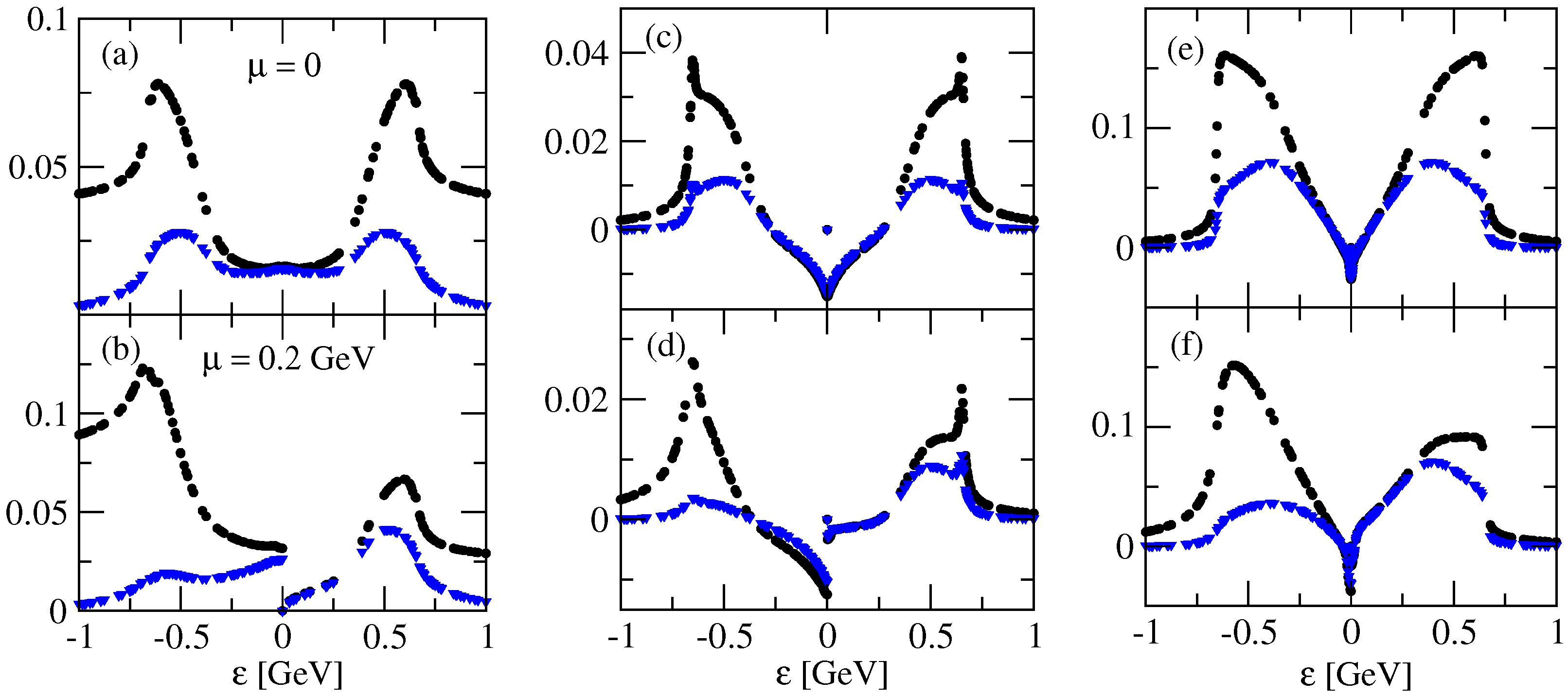
Figure 3.
The integrands of the integral : (a) the inner integrand as a function of quark momentum at various values of and (shown in GeV units); (b) the p-integral of (solid lines, in GeV units) and its product with the factor (dashed lines) as functions of for various values of : , and GeV.
Figure 3.
The integrands of the integral : (a) the inner integrand as a function of quark momentum at various values of and (shown in GeV units); (b) the p-integral of (solid lines, in GeV units) and its product with the factor (dashed lines) as functions of for various values of : , and GeV.
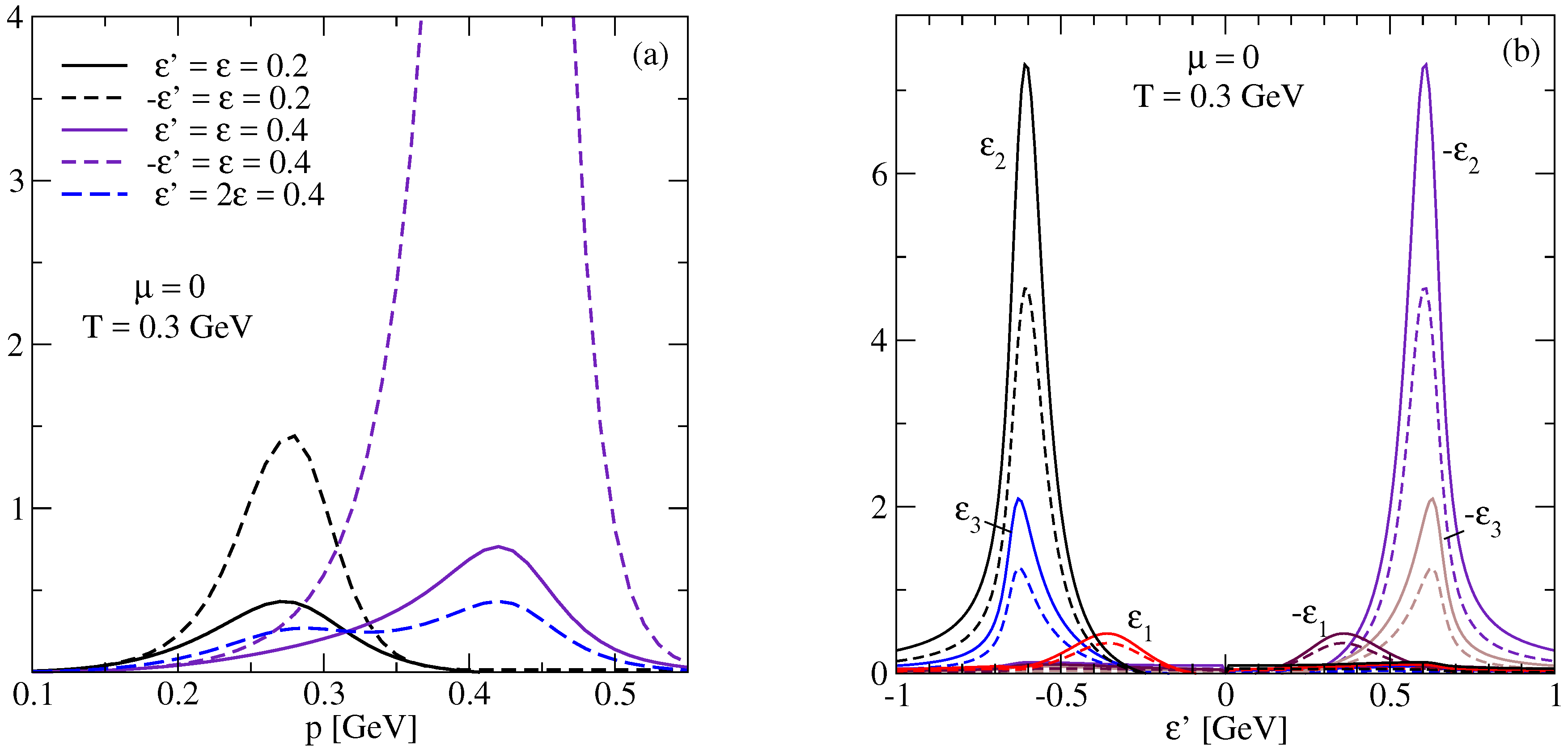
Figure 4.
Dependence of the integrals (a), (b), (c) and the renormalized coupling (d) on the temperature for several values of the chemical potential. The corresponding Mott lines are shown by vertical lines. The value of the bare coupling constant G is shown by the solid horizontal line.
Figure 4.
Dependence of the integrals (a), (b), (c) and the renormalized coupling (d) on the temperature for several values of the chemical potential. The corresponding Mott lines are shown by vertical lines. The value of the bare coupling constant G is shown by the solid horizontal line.

Figure 5.
The contributions of the single-loop () and multiloop (, ) diagrams to the bulk viscosity, as well as their sum as functions of the temperature for vanishing (a) and finite (b) chemical potential. The dotted lines correspond to the chiral limit . The results of the fit formula (74) are shown by circles.

Figure 6.
The ratio as a function of the temperature for several values of the chemical potential. The corresponding ratios are shown for comparison by crosses. The solid horizontal line shows the KSS bound [2].
Figure 6.
The ratio as a function of the temperature for several values of the chemical potential. The corresponding ratios are shown for comparison by crosses. The solid horizontal line shows the KSS bound [2].
© 2018 by the authors. Licensee MDPI, Basel, Switzerland. This article is an open access article distributed under the terms and conditions of the Creative Commons Attribution (CC BY) license (http://creativecommons.org/licenses/by/4.0/).
Share and Cite
MDPI and ACS Style
Harutyunyan, A.; Sedrakian, A. Bulk Viscosity of Hot Quark Plasma from Non-Equilibrium Statistical Operator. Particles 2018, 1, 212-229. https://doi.org/10.3390/particles1010016
AMA Style
Harutyunyan A, Sedrakian A. Bulk Viscosity of Hot Quark Plasma from Non-Equilibrium Statistical Operator. Particles. 2018; 1(1):212-229. https://doi.org/10.3390/particles1010016
Chicago/Turabian StyleHarutyunyan, Arus, and Armen Sedrakian. 2018. "Bulk Viscosity of Hot Quark Plasma from Non-Equilibrium Statistical Operator" Particles 1, no. 1: 212-229. https://doi.org/10.3390/particles1010016