An Adaptive Ensemble Approach to Ambient Intelligence Assisted People Search
by
 , , , and
Dongfei Xue
1 ,
,
Xiaonian Wang
2,
Jin Zhu
2,
Darryl N. Davis
1,
Bing Wang
1,
Wenbing Zhao
3 ,
,
Yonghong Peng
4 and
and
Yongqiang Cheng
1,* 1
School of Engineering and Computer Science, University of Hull, Hull HU6 7RX, UK
2
Department of Control Science and Engineering, Tongji University, Shanghai 201804, China
3
Department of Electrical Engineering and Computer Science, Cleveland State University, Cleveland, OH 44011, USA
4
Faculty of Computer Science, University of Sunderland, St Peters Campus, Sunderland SR6 0DD, UK
*
Author to whom correspondence should be addressed.
Appl. Syst. Innov. 2018, 1(3), 33; https://doi.org/10.3390/asi1030033
Submission received: 13 July 2018
/
Revised: 23 August 2018
/
Accepted: 28 August 2018
/
Published: 3 September 2018
(This article belongs to the Special Issue Healthcare System Innovation)
Abstract
:Some machine learning algorithms have shown a better overall recognition rate for facial recognition than humans, provided that the models are trained with massive image databases of human faces. However, it is still a challenge to use existing algorithms to perform localized people search tasks where the recognition must be done in real time, and where only a small face database is accessible. A localized people search is essential to enable robot–human interactions. In this article, we propose a novel adaptive ensemble approach to improve facial recognition rates while maintaining low computational costs, by combining lightweight local binary classifiers with global pre-trained binary classifiers. In this approach, the robot is placed in an ambient intelligence environment that makes it aware of local context changes. Our method addresses the extreme unbalance of false positive results when it is used in local dataset classifications. Furthermore, it reduces the errors caused by affine deformation in face frontalization, and by poor camera focus. Our approach shows a higher recognition rate compared to a pre-trained global classifier using a benchmark database under various resolution images, and demonstrates good efficacy in real-time tasks.
1. Introduction
To facilitate proper robot–human interactions, an immediate task is to equip the robot with the capability of recognizing a person in real time [1,2]. With the development of deep learning technology and the availability of larger image databases, it is possible to achieve a very high facial recognition rate using some benchmark databases; for example, 95.89% for the Labeled Faces in the Wild (LFW) database [3], and a slightly lower recognition rate of 92.35% after projecting the images into 3D models [4]. However, such algorithms are not directly usable for facial recognition in real-world scenarios, because faces should also be recognized from the side, which are heavily affected by affine deformation in 3D alignment, and, from a long distance, the captured face image could be of poor quality and low resolution.
Another main challenge for the facial recognition system is “poor camera focus” [5,6]. When the distance from the camera to the subject is increased, the focal length of the camera lens must be increased proportionally if we want to maintain the same field of view, or the same image sampling resolution. A normal camera system may simply reach its capture distance limit, but one may still want to recognize people at greater distances. No matter how the optical system is designed, there is always some further desired subject distance, and, in these cases, facial image resolution will be reduced. Facial recognition systems that can handle low-resolution facial images are certainly desirable.
We believe that humans benefit from the smaller sized facial database maintained in their memory for people recognition and identification [7,8]. Humans can fully utilize local information such as location and prior knowledge of the known person (e.g., characteristic views), which makes them capable of focusing their attention on more obvious features that are easier to detect [9,10].
For example, when a person searches for an old man from a group of children, grey hair might be an apparent feature that can be recognized from a far distance and in different directions. Conversely, when a person looks for a young boy from a group of children, hair color might be trivial. Different features should be selected for recognition tasks amongst different groups of people, depending on our prior knowledge of the known person.
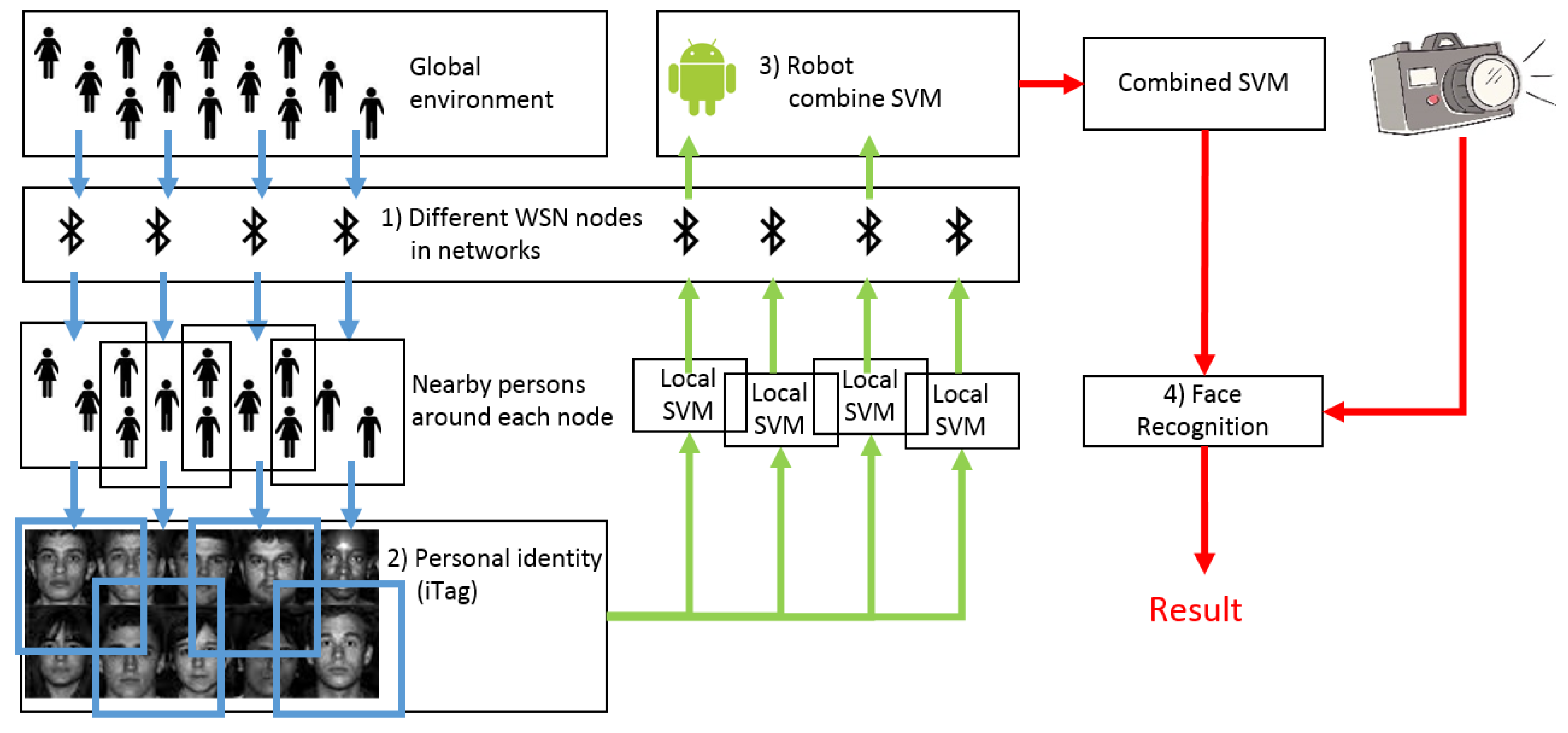
In this article, we propose an adaptive ensemble approach to improve facial recognition rates, while maintaining low computational costs by combining a set of lightweight local binary classifiers with pre-trained global classifiers. In this approach, we assume that the physical world is covered by a wireless sensor network (WSN) that is comprised of multiple wireless communication nodes. They are distributed in the environment and are aware of local context changes, such as when people come into or depart from its vicinity. Each node maintains a lightweight classifier to best distinguish nearby people. Features of new people are learned by the node as they enter into the communication range of a node, even if only one photo per person is available for training. The robot can collect the lightweight classifiers from the nodes on its way. These lightweight classifiers will then be combined with other pre-trained global classifiers by the robot to find the right features for facial recognition.
Our method has been tested in a real-world experiment. Each WSN node is a “Raspberry Pi3” credit card-sized computer. The pioneer robot (Pioneer 2-DX8 produced by ActivMedia Robotics, LLC., Peterborough, NH, USA) is used to search people and to recognize them based on snapshots. Figure 1 is an overview of our proposal.
The combination of a real-time learnt lightweight local binary classifier with pre-trained global classifiers addresses the extreme unbalance of false-positive results when the classifier is used in local dataset classifications. Furthermore, it reduces the errors that are caused by affine deformation in face frontalization. We describe the problems using a linear classifier model, and we further strengthen the validity of the proposed solution using the Gaussian distribution model. The Fisher’s linear discriminant is applied to estimate the marginal likelihood of each classifier against the target. Finally, posterior beliefs are used to orchestrate the global and local classifiers.
The proposed method has been implemented and incorporated into a robot and its operating environment. In our real-time experiments, the robot exhibits a fast reaction to the target. It adjusts its face recognizer to detect facial features effectively by focusing its attention on the persons in its vicinity. Compared with the results that are obtained in our approach and a single pre-trained classifier in respect to some benchmark databases, our approach achieves a higher facial recognition rate and a faster facial recognition speed. The contributions of the paper can be summarized as below:
- (1)
- A new adaptive ensemble approach is proposed to improve facial recognition rates, while maintain low computational costs, by combining lightweight local binary classifiers with global pre-trained binary classifiers.
- (2)
- The complex problem of real-time classifier training is simplified by using locally maintained lightweight classifiers among nearby WSN nodes in an ambient intelligence environment.
- (3)
- Our method reduces the errors caused by the affine deformation in face frontalization and poor camera focus.
- (4)
- Our method addresses the extreme unbalance of false positive results when it is used in local dataset classifications.
- (5)
- We propose an efficient mechanism for distributed local classifiers training.
The rest of the paper is organized in the following sections. Some background knowledge is given in Section 2. Theoretical analysis of the problem using Gaussian distribution models and an ensemble of the pre-trained classifiers with their posterior beliefs are described in Section 3. Section 4 details the proposed people search strategy, utilizing a single photo of the front face. Section 5 presents our real-time experiments. Section 6 concludes the paper.
2. Related Work
2.1. Facial Recognition
A typical facial recognition system [11] is an open-loop system, comprised of four stages: detection, alignment, features encoding, and recognition. In an open-loop system, there is no feedback information drawn from its output. This means the recognition process highly relies on prior knowledge, i.e., the pre-trained features and classifiers.
Deep-learning methods, e.g., Facebook Deepface, supply us with very strong features under different conditions. Deepface shows very high accuracy (97.35%) on the benchmark database LFW [12]. This performance improvement is attributed to the recent advances in neural network technology and the large database that is available to train the neural network. Deepface encodes a raw photo into a high dimensional vector, and it expects a constant value for a given person as an output. Despite the high accuracy that is achieved by applying the deep-learnt features and binary classifiers, three main issues remain when implementing them for real-time applications:
- (1)
- Image features are extracted on the aligned face photo, but the face alignments of different people are based on a common face model. This causes unexpected errors during affine transformation. This kind of error is further enlarged when we apply a 3D frontalization method [4] onto the low-resolution photos. For example, Figure 2 shows the front and side faces of a male. Figure 2A,C has high resolutions, hence the frontalization of the photos shows no sign of information loss; we can see the large degree of deformations on the estimated front face (Figure 2F,H), from the low-resolution photos (Figure 2E,G, respectively). Especially Figure 2H is inclined to show the female features.
- (2)
- A binary classifier is usually used as the face recognizer, which is trained to distinguish between two photos belonging to the same person. Because only one or a limited number of photos per person are available to train the recognizer, and due to the over-fitting problem [13] in machine learning, a binary classifier usually achieves a better result than a multiclass classifier. Consequently, heavily unbalanced results ensue, i.e., much more false results occur on positive samples than on negative ones [14]. In a real-time application, we are more concerned about the correctness of the positive samples.
- (3)
- Global classifiers are trained using web-collected data, which are very different to the images that are captured by robots in daily life.
2.2. Ambient Intelligence
An ambient intelligence environment, also known as a smart environment, pervasive intelligence, or robotic ecology [15,16,17], is a network of heterogeneous devices that are pervasively embedded in daily living environments, where they cooperate with robots to perform complex tasks [18,19].
Ambient intelligence environments utilize sensors and microprocessors residing in the environment to collect data and information. They generate and transform information that are relayed to nearby robots, and they can be helpful in a variety of services; for example, to estimate the location of an object via the triangulation method [20] by sensing the signals from anchor sensors, or to share a target’s identity information by broadcasting or enquiring through wireless communication. This will either offload or simplify traditionally challenging tasks such as localization and object recognition, which are otherwise performed in a centralized standalone mode through the utilization of environmental intelligence. This potential makes them increasingly popular, especially for indoor applications.
3. Adaptive Ensemble of Classifiers
3.1. Problem Statement
Assume that there is a set of lightweight classifiers , pre-trained in advance, for facial recognition, where denotes the index of the classifiers, and is an N-dimensional feature vector. Each is trained using different data subsets. The datasets of training samples for each may vary with respect to number, size and resolution. A robot is given the task of selecting the best combination of the classifiers to correctly distinguish a person from a smaller dataset when supplied with only a face photo of that person at run time. The smaller dataset could be a group of people surrounding the robot, or its localized environment, with the robot being informed of their existence by devices that respond to tags that they are wearing. The key problem is to find the right relational model between any specific target photo and the optimized ensemble of the classifiers .
3.2. Assumption
We assume that the facial features of any can be described with Gaussian distribution models [21] with standard deviation , as shown in Equation (1):
is an N-dimensional feature vector, which is extracted from a front face photo for the WSN node to learn of a new person, and is an input sampled from previously known images for comparison.
describes the degree of difference between two photos that may appear for the same person. This is learned from training samples, and each may have different , represented as . Assuming that facial features are independent from each other, we can derive Equations (2) and (3):
where represents a single feature among , denotes an atom in vector , and is one of the diagonal elements in . Our decision function can be written as Equation (4):
This means that two photos are from the same person if , otherwise they are not (). and are two sets of features from different parts of a face. embodies the features that change substantially between two different people; measures the changes among different head poses for the same person. The value is a scalar parameter between these two Gaussian distributions.
3.3. Decision Function
Given that and are two sets of different features, if the feature number of is , and the feature number of is , they can be written as below:
To simplify the decision function and to express our question more clearly, we can write and as a proportion (Equation (7)):
Let and . Because and embody two sets of different features on the face, i.e., and , it can be simplified as below:
where . Hence, Equation (7) can be simplified as Equation (9):
If we substitute the above into Equation (4), then becomes as follows:
By reorganizing the above equation, we have:
Then:
Then:
Letting , we have obtained the decision function from Equation (4) as follows:
where is a threshold parameter related to , and is a linear function. Each weight parameter of is determined by the standard deviation of , which is independent and can be adjusted separately.
3.4. Linear Function Solution
In our decision function (Equation (10)), is a linear function. Given any linear function such as Equation (11), its parameters and can be solved by support vector machine (SVM) [22] decomposition, which tries to find a hyperplane to maximize the gap between two classes, as shown in Equation (11):
It is straightforward to solve a single decision function (Equation (10) by applying the method of SVM on Equation (11). Our problem is how to combine multiple decision functions from different classifiers.
3.5. Classifier Combinations
Using different datasets for training, we may obtain different classifiers, so that in Equation (11) for classifier m, its decision function can be represented as Equation (12):
When we give a robot a front face photo to learn the features of a new person, we are looking for a mixture matrix , as in Equation (13), to combine the pre-trained classifiers to obtain a higher recognition rate. Equation (14) is a combination of M classifiers, where () means the Hadamard product (entrywise product):
where is the combined classifier that we are looking for. The result of represents the combined features of the new person obtained, by adjusting the weight parameter using , and similarly tuning threshold using .
3.6. Estimation of the Mixture Matrix
To combine the multiple decision functions, we need to properly estimate the mixture matrix in Equation (13). According to the Bayesian model, we can combine classifiers by their posterior beliefs, as in Equation (15):
where and are one atom from feature vectors and , respectively. is one of the weight parameters of the classifier , which measures the distribution of .
Equation (15) is comprised of two parts:
- (1)
- is an unknown value. We decompose it further as Equation (16), where is the prior belief of each classifier. is the marginal likelihood for under the distribution of .
- (2)
- is a conditional probability. In our decision function (Equation (10)), each feature from vector gives its vote on the final decision independently. We simply estimate it by:
By substituting Equation (17) into Equation (14), it becomes:
Comparing the above equation with Equation (15), it is easy to see that there exists a one-to-one relation between and . This can be formally written as Equation (19):
Each element in the mixture matrix A can be calculated through Equation (16). Here, the prior belief of each classifier is a known value, and it can be obtained by verification on a set of test samples. is a constant value for all , but the marginal likelihood is hard to estimate because is a single sample.
3.7. Estimating Marginal Likelihood
According to Fisher’s linear discriminant [23], a good classifier shows a large between-class scatter matrix and small within-class scatter matrix.
For facial recognition, a within-class scatter matrix measures the changes on the images of people due to changes in head pose and illuminations, while between-class scatter relates to changes in the image subject. This suggests that the quality of the classifier is highly determined by the between-class scatter matrix, given the same pose and illumination conditions. In other words, the data distribution could be more consistent with classifier’s estimations, provided that each is far enough from the mean value, i.e., the mean face.
Hence, the marginal likelihood can be measured as the distance between and the mean value in the training samples. For a different classifier , its mean value may vary, because the classifiers may be trained on a different sample set. Let denote the features of the training samples for ; if is one atom from the face vector, and is the number of training samples, then can be calculated by:
Let denote the variances of ; it can be written as:
If given a new face photo for training, is one atom of its face feature vector, and we can estimate as below:
Equation (22) suggests that the mean face must obtain the worst result (recognition rate) on each classifier, and that the photo for that position cannot be distinguished among other people, because it looks like (or unlike) anyone.
3.8. The Outline of Our Method
The main steps of our proposed method are outlined as below:
- (1)
- Multiple classifiers are pre-trained for facial recognition in advance; each one is determined by the linear function (Equation (10)).
- (2)
- Each WSN node maintains a to distinguish between a small number of nearby people. The robot collects a set of from WSN nodes on the way.
- (3)
- One face photo, of the target person is provided for recognition. The combinations of are adjusted with the input of in order to correctly distinguish this person.
- (4)
- The classifiers are orchestrated by mixture matrix A in Equation (14), which is a matrix of conditional possibility, as shown in Equation (19).
- (5)
- The likelihood is estimated by measuring the distance between and the mean value , as seen in Equation (22).
- (6)
- Finally, mixture matrix A can be calculated as Equation (16), and is normalized as below:
From the above analysis, a relational model was derived to represent the link between a specific sample and the pre-trained classifiers, based on conditional probability and Fisher’s linear discriminant. This provides a novel way to adjust the combination of pre-trained classifiers according to the selected target . The model is also capable of adapting to low resolution images with resized by a corresponding mixture matrix A, to find the best features on low-resolution images.
4. Evaluation with Benchmark Databases
We evaluated our algorithm on the LFW and YaleB benchmark databases. Two experiments were carried out to compare our method with other linear and non-linear binary classifiers. Firstly, we compared our method with a single SVM that was trained on a large-sized database; in this experiment, we wanted to show that our method could obtain a higher overall recognition rate and a lower false positive rate than a pre-trained classifier. Some other binary classifier models (i.e., quadratic discriminant analysis [24] and logistic regression [25]) were also considered in the experiment. Secondly, we compared our method with SVM that were trained on small-size databases for local people, through in this experiment we wanted to show that our method could combine local classifiers when the database size was small, and when the data samples were partially overlapped.
4.1. Benchmark Database
The LFW database is a database of facial images created by the University of Massachusetts for a study on unconstrained facial recognition [26]. The dataset contains 13,233 photos of 5749 people, which are collected from the web. Most of these photos are clear, but with random head poses and under different illumination conditions. The average size of the photos is 250 × 250 pixels.
The YaleB database contains 16,128 images of 28 people [27]. The photos are well organized and are sorted under nine poses and 64 illumination conditions. In our experiments, we studied the photos of the nine head poses under good illumination conditions, where the filename ended with the suffix “000E+00.pgm”.
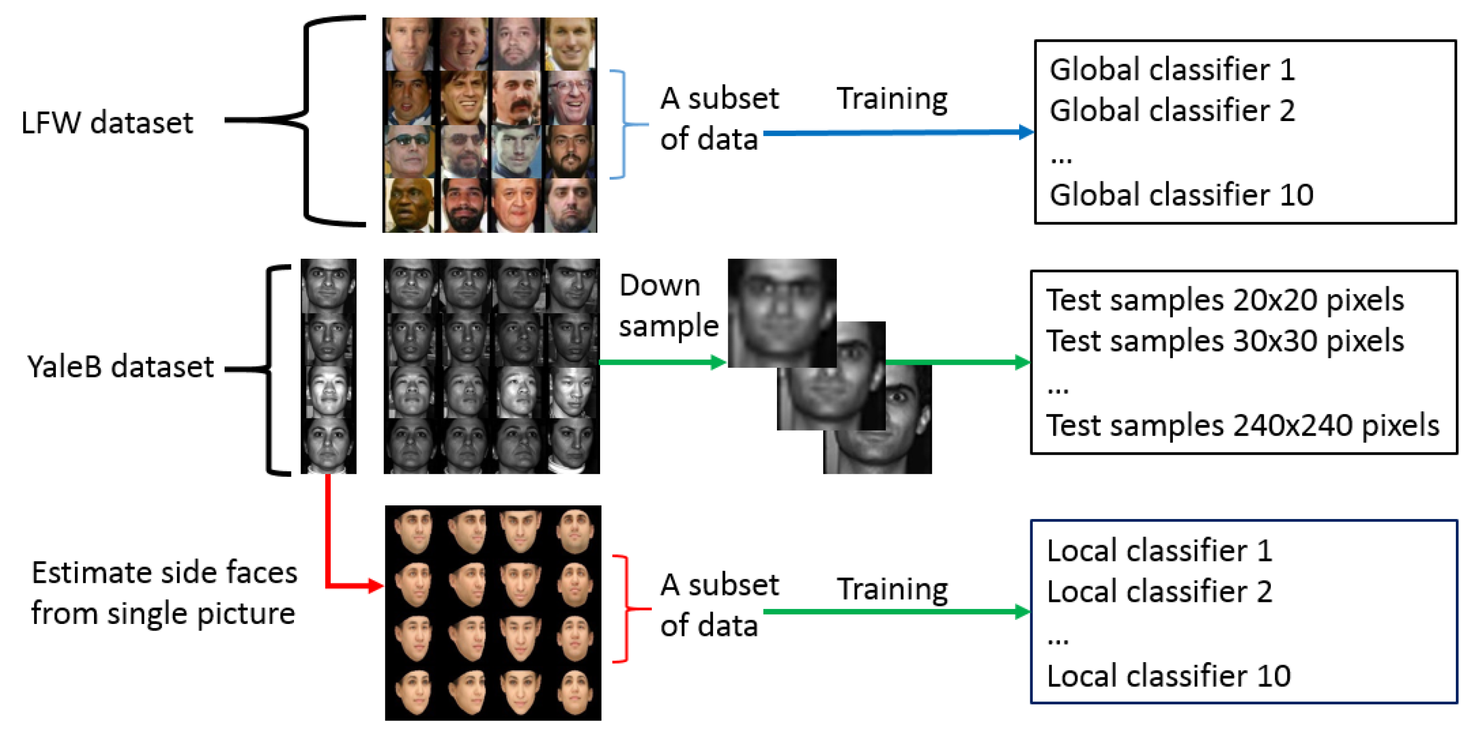
Our global classifiers were trained on the LFW database. The LFW separates all of the data into 10 subsets, and each set contains 5400 samples for training. We trained the classifiers on each subset of LFW, and we obtained 10 different global classifiers, as detailed in Figure 3.
The classifiers were tested on the YaleB database. Because each person showed nine different head poses in YaleB, 252 photos were obtained for verification. After randomly pairing these photos, we selected 378 positive samples (two photos from the same person) and another 378 negative samples (two photos from different people). The face photos were down-sampled to different resolutions in advance. It obtained six different datasets of resolution from 20 × 20 to 240 × 240 pixels.
Local classifiers were trained on the YaleB database. One photo per person was selected from YaleB, and a total of 28 front face photos (P00A+000E+00.pgm) were obtained for training. These 28 photos were separated into 10 overlapped sets of 14 people, and the local classifiers were trained on each set. Details can be found in the section below.
4.2. Data Pre-Processing
LFW is a relatively large database of face photos, and it provides enough samples for training, while YaleB is much smaller. Since the available 28 YaleB front face photos were not enough to train classifiers, we had to expand the training samples by estimating the person’s side faces using a 3D morphable model (3DMM) [4].
3DMM is a 3D tool based on a deep-learning method, and it can extract facial features from a photo. 3DMM face features embody a 3D face model. Using 3DMM, a front face photo in the YaleB database can be expanded by projecting the single face photo into 15 different poses, i.e., [0, 15, 30] degree in the horizontal direction, and [−30, −15, 0, 15, 30] degrees in the vertical direction. This generated an extra 14 samples per person for training (excluding the original front face). By randomly pairing the 3DMM estimated faces, it obtained 6000 samples for training. Among them, 3000 were positive samples (two photos from the same person) and another 3000 were negative samples (two photos from different people).
There were 283,638 face features extracted from each photo by 3DMM running on the “Caffe” deep learning framework. Let denote the face features of one photo; denotes the face features of another photo. The classifier was trained to distinguish whether the two face photos were from the same people. The difference between and was taken as the observed value, as shown in Equation (12). In our experiment, the observed value was compressed into a 100-bit vector using principal component analysis (PCA) method [28].
4.3. Classifier Combinations
Given a face photo of target person, we combined the classifiers by adjusting the mixture matrix to combine classifiers, as shown in Equation (14). The only unknown value was the prior belief for each classifier. The global classifier was trained on a large LFW database with 5400 samples. The LFW database also provided another 600 samples for verification. We took the recognition rate as the prior belief for each global classifier.
The local classifier was trained on a small YaleB database. We used the same database for training and verification, and we took the recognition rate as the prior belief for each local classifier. The local classifier usually obtained a higher prior belief value than the global one.
The mixture matrix was adjusted for different target people, to highlight the important face features. In a linear classifier (Equation (10), the important features should receive a large weight value . It was easier to understand our idea, if we drew all of the facial features on a figure. The 3DMM face features contain face shape information in a matrix of 24,273 × 3; each column is a triple-element in the XYZ format. If this shape information is used to train a linear classifier, it can obtain a 24,273 × 3 weight value . With all of the drawn onto a figure, the result looks like a face mask, as in Figure 4.
Figure 4 shows the strategy of the classifier to distinguish targets from 28 YaleB people. The blue areas are the positions of the largest (top 10%) positive weight values , and the red areas are the positions of the smallest negative values . The figure shows that Global SVM extracted more large values of on the eyebrow area, whilst the local SVM focused on the jaw area. It is interesting to note that the local SVM picked up many points in the nose wing area, while the global SVM nearly completely ignored that area.
Our method adaptively used different linear classifiers for different targets when combining the global SVM and local SVM classifiers. As shown in Figure 4, the nose wing area was selected by our method for the target boy “YaleB33”, as this was an apparent feature for recognizing this person. However, for the case of the target girl “YaleB27”, nose wing area should not be considered as an apparent feature. This was also consistent with the strategy that is normally adopted by a human, i.e., a focus on more apparent features such as a tall nose bridge for recognizing the target boy “YaleB33”, but not the girl “YaleB27”.
4.4. Experiment Result on the Benchmark Database
Through the above examples, it was found that our method could adapt its strategy to distinguish between different targets. In real situations, the facial features were represented as an array of vectors, and they could not be drawn on a figure. The 3DMM face features were compressed into 100 bit vectors before training and testing. Twenty SVM classifiers were combined in our experiment; 10 of them were trained on the LFW database, and the other 10 were trained on the YaleB database.
Two experiments were conducted in this section to validate the performance of our method. Firstly, we compared our method with some other linear and non-linear classifiers. The algorithms of quadratic discriminant analysis (QDA), SVM, and logistic regression were trained on the LFW database. Then, they were tested on the YaleB database, and the results are compared in the below Table 1 and Table 2.
The results in Table 1 show that our method achieved a higher recognition rate for both the medium-sized photos (240 × 240 with 93.21% success rate) and small-sized photos (30 × 30 with 88.96% success rate). The average recognition rate of our method was 89.87%, which was higher than the SVM (85.94%), QDA (85.49%), and logistic regression (80.38%) methods. The false positive rate shown in Table 2 was also very limited by our method, at 11.56%. In contrast, global classifiers were inclined to obtain more false positive results (above 20.90%).
In our second experiment, the YaleB database samples were separated into smaller sets of 10 people, or into bigger sets of 18 people, and each set contained different overlapped people. The results are listed in Table 3. It showed no apparent decline in performance when the number of overlapped data decreased. When 75% of the data were overlapped between YaleB subsets, a single local SVM classifier obtained an 85.57% recognition rate. When only 35% of the data were overlapped, the recognition rate of a single SVM classifier slightly declined to 84.93%. In contrast, our method maintained a higher recognition rate of around 88.76% in all cases. Our method also kept lower false positive rates, of below 12.35% as shown in Table 4.
5. Real-World Experiments
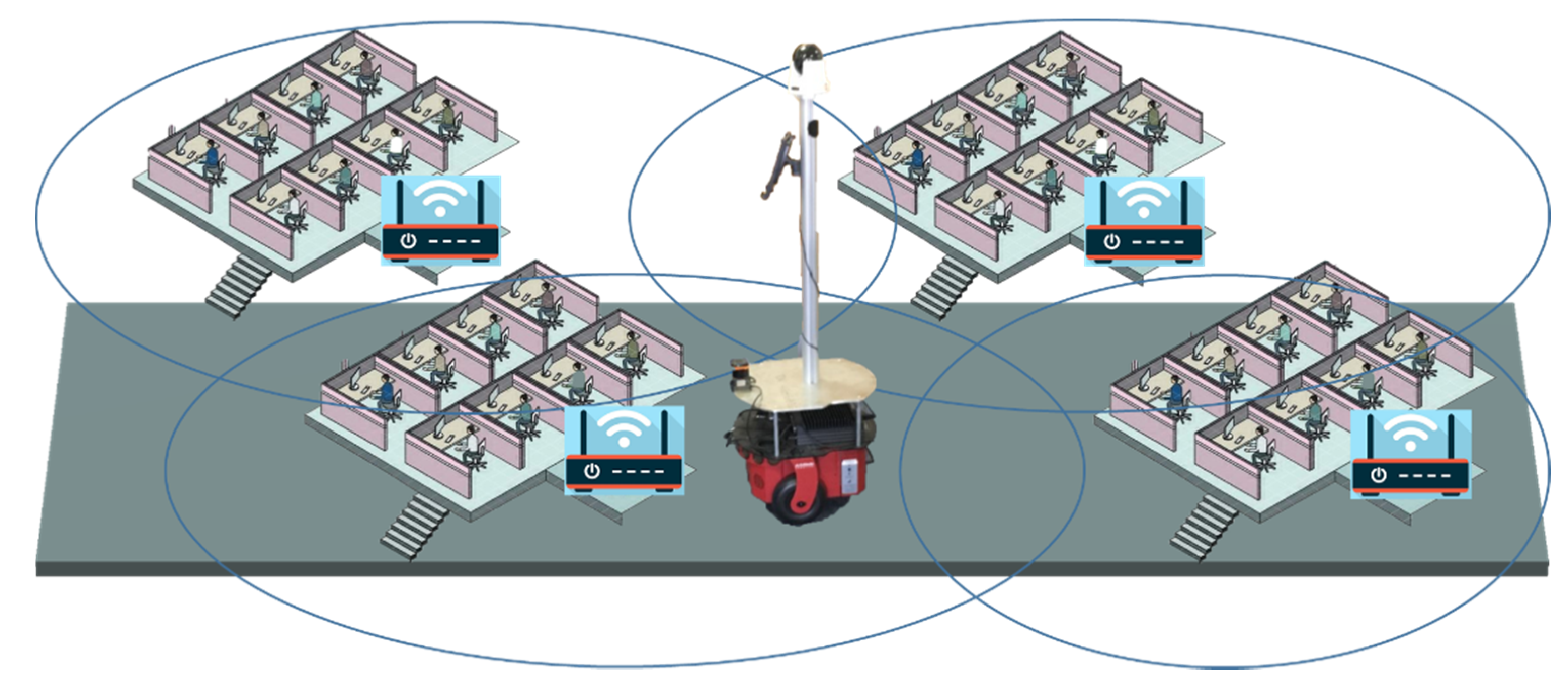
In our experimental environment, three kinds of smart devices were deployed, as shown in Figure 5:
- (1)
- Nodes: Both Bluetooth low-energy (BLE) and Ethernet-enabled gateway devices were mounted on the walls at each corners of the room. We used “Raspberry Pi3” as WSN nodes in the experiment. They continuously monitored other BLE devices activities and communicated with the robot wirelessly. Each WSN node maintained a lightweight classifier to recognize nearby people within its communication range.
- (2)
- iTag: These are battery powered BLE enabled tags. We used “OLP425” in the experiment, which is a BLE chip produced by U-blox. The OLP425 tags are small in size, with limited memory and a short communication range of up to 20 m. They support ultra-low power consumption, and they are suitable for applications using coin cell batteries. Each iTag saves personal information such as a name and a face photo in their non-volatile memory, and it accepts enquiries from the WSN node.
- (3)
- Robot: The robot is a Pioneer 2-DX8-based two-wheel-drive mobile robot and it contains all of the basic components for sensing and navigation in a real-world environment, including battery power, two drive motors, and a free wheel, and position/speed encoders. The robot was customized with an aluminum supporting pod to mount a pan/tilt camera for taking snapshots of people’s faces for the recognition tasks. A DXE4500 fanless PC with Intel core i7 and 4 GB RAM on board with wireless communication capability handles all the processing tasks, including controlling and talking to the WSN nodes.
The model of the camera on the robot is “DCS-5222L”, which supports a high-speed 802.11 n wireless connection. The snapshot resolution is fixed at 1280 × 720 pixels. When people were nearer to the camera (within 4 m), the face area was clear and occupied a large number of pixels (240 × 240) in the camera view. When people were further from the camera (around 10 m away), the face region in the camera view became smaller and blurrier, with approximately 30 × 30 pixels.
Figure 5 shows the system structure of our experimental environment. People were required to wear the iTag when they were working in this environment. Each iTag saved the personal name and face photo of its owner in its memory. WSN nodes were distributed in the physical world. The signal of each node was not strong enough to cover the whole environment, due to their limited wireless communication range. Each WSN node took care of a small area in its vicinity, so that the physical world was sectioned into smaller areas that were under the control of different WSN nodes.
The WSN nodes were responsible for searching for the existence, approach, and departure of iTags in its vicinity. Each node scanned nearby iTags through Bluetooth communication continuously. Once it found a new iTag signal, it downloaded the personal name and face photo from iTag. It trained and maintained a local classifier to recognize a small number of nearby people. One person could be detected by multiple WSN nodes at the same time, so that people may be used in different classifiers.
Figure 6 shows the processing flow of the robot. When a robot received a command from an operator to search for a person in our experiment environment, the iTag ID or the name of the target was given. The robot enquired to the WSN about the details of this target by supplying this iTag ID or name. The enquiry was broadcasted through the entire WSN by multi-hop routing. If the target was seen by the WSN nodes, they would respond to the robot with a face photo of the target. The robot then exchanged messages with those WSN nodes about the position of target if the target was still in their vicinity. The robot could receive multiple replies if the target was in the range of multiple nodes.
If the robot did not find the target from a distance, it went to the next region covered by a different WSN node that replied its enquiry. If the target was identified in the view of the robot’s camera and verified by second-round recognition at a closer distance, the robot ended the search task and sent an indication to the operator and to the target people. If the robot found that the target did not match the given information, then it ended the task and informed the operator with a failure message.
A global map was constructed using a grid-based simultaneous localization and mapping (SLAM) algorithm with Rao-Blackwellized particle filters [29,30] implemented in an open source software ROS gmapping package. The map was constructed in advance and it was stored on the robot. The coordinates of each WSN node were also marked on the map as anchor nodes for preliminary target localization. The robot used a sonar and laser ranger to scan for environmental information for map building, as well as for locating itself on the map. The robot visited the WSN nodes one by one if it received responses from multiple nodes. When the robot moved into a region that was controlled by different WSN nodes, it collected local lightweight classifiers from the node and combined them with the global classifiers stored in the robot for facial recognition. After the robot reached the control region of a target node, it used its camera to scan the area. The facial recognition process was a two-phase process. After the first round of facial recognition, it moved towards a closer position to take another snapshot of the face and then it performed a second round of recognition to reconfirm the result.
In a real-world experiment, we stored the YaleB database and our researchers’ face photos, respectively, on 30 iTags. The robot was started from different distances to compare the performance of our method with the single pre-trained SVM classifier. Ten local classifiers and 10 global classifiers were combined; the parameters of the classifiers were the same as in Section 4.1. The experiment results can be found below.
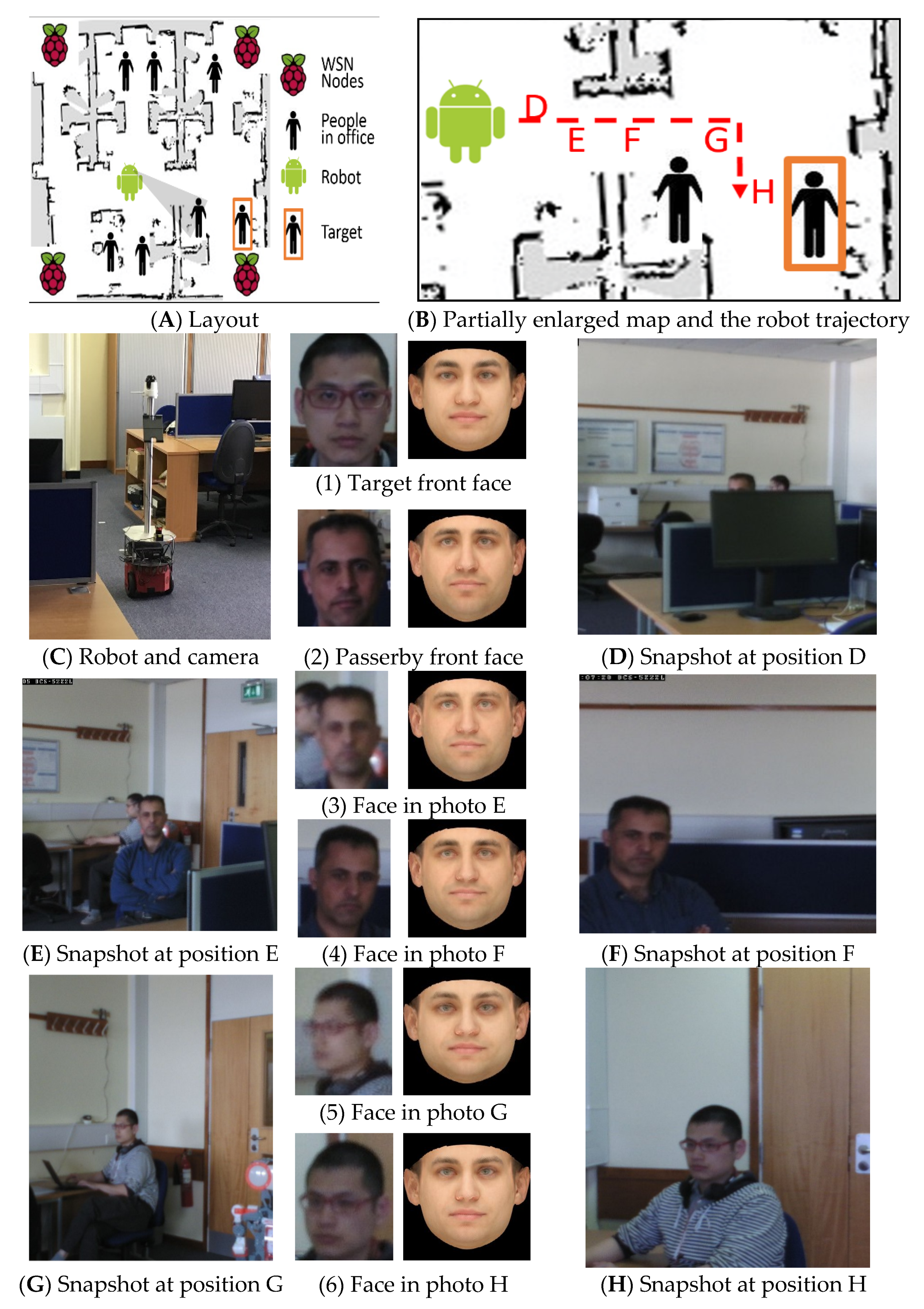
In our real-time application, the wireless sensor environment helped to simplify the tasks for the robot, and made it focus more specifically on a small group of people in the vicinity. The location of the iTags could be estimated, and their identities were broadcast across the environment. When the WSN node detected a new face, it took around 11 s to expand a single face photo to nine different poses using the 3DMM method, and around 6 s to train the local SVM classifier. No apparent time delays occurred during facial recognition. Given the feature vector of a face photo, the robot could combine classifiers and output the results within 5 ms. The robot was fully prepared to recognize all of the people in the environment; meanwhile, it monitored a specific area rather than looking around randomly. Figure 7 shows the details of our experiments:
- (A)
- Office layout and the wireless sensor environment. Guided by the WSN node information, the robot searched the bottom right area of the displayed map.
- (B)
- Partially enlarged map and the robot trajectory.
- (C)
- The robot with the pan/tilt camera on its top.
- (D)
- A snapshot at position D. Blocked by the computer screen, robot did not find anyone. Photo 1 is the target person and his frontalized photos by 3DMM. Photo 2 is one of our colleagues. Another 28 face photos for training and recognition came from the YaleB database.
- (E)
- A snapshot at position E. One face was detected at a distance of three meters (photo 3). Though it was very low in resolution, our method gave negative votes, because it was not the target person.
- (F)
- A snapshot at position F. For a moving robot, faces may occur at the corner of the snapshot photo, and they may be easily missed (Photo 4).
- (G)
- A snapshot at position G. The target was detected and classified as a true positive by our method with the combined SVM; this would otherwise have been classified as a negative result by the single global SVM approach.
- (H)
- Moving forward to position H, and a better quality face photo was obtained. The robot finally found the target people.
We compared our method with a single pre-trained SVM in real-world experiments. The robot was asked to search for people in an office. It moved at 0.2 m/s indoors, and spent around 150 s to create a full view (13 snapshots at 340° rotation) of the surrounding environment. The results were based on 24 experiments, and can be found in Table 5.
In real-world implementations, our locally assembled face recognizer obtained a stable and good result for facial recognition. It could find targets in low quality photos caught from a far distance, and the recognition rate was 80% at around 9 m. Meanwhile, it took fewer snapshots and facial recognition processes, because the false positive recognition rate was kept at a relatively low level. Equipped with our face recognizer, the robot could detect people from a far distance, so that it did not have to move near people to obtain a better line of sight every time. Moreover, it also saved much time by avoiding mistaken identities.
In contrast, when we used a single pre-trained SVM as the face recognizer, the robot recognized the wrong people, and it spent more time approaching the wrong target. The side face photo may have contained affine deformation, especially when it appeared near the photo frame. The camera needed to rotate slowly to obtain a target-centered photo. Once it missed the target, the robot needed to carry out a complete search again, that was why a single pre-trained SVM took more snapshots and spent more time on facial recognition than our method in the experiment.
Although our method also met the problem of distorted face photos, our locally combined binary classifier correctly selected the face features, and it showed better recognition rate for familiar people in its vicinity.
6. Discussion
A robot vision system needs to overcome similar situations that a human visual system may have in daily life. However, it pays very high computational costs to fulfil the task, especially when it suffers from ill-posed views, wheel slippage, movement vibrations, and accident recovery. The following are some examples of constraints placed on the system:
- (1)
- The quality of the photo is heavily affected by the body pose of the robot. Most laboratory robots are not tall enough to get a human-level view. The Pioneer 2-DX8 robot used in the experiment is lower than 27 cm. A one-meter tall rod was used to raise the camera on top of the robot body frame (Figure 7C).
- (2)
- A surveillance camera has a limited visual range. For example, the face area viewed by the camera is around 40 × 40 pixels at a 10 m distance, which is too small to be recognized. The cloud camera (DCS-5222L) was taken as the camera source for the robot in our project. Its rotation range is 340°, and highest photo resolution is 1280 × 720 pixels. Most of the face images acquired were side views, and the quality of some photos were poor with low resolution. Hence, in the experiment, multiple snapshot candidates had to be taken to increase the quality.
- (3)
- To stabilize the camera on its top, the robot cannot move too fast. Furthermore, it has to wait for the camera to stop rotating before it can acquire a clear image.
- (4)
- Limited by its view and line of sight, a self-controlled robot cannot get a good overview of the whole area. It has to patrol around the room step-by-step to search for the target if no location hypotheses from ambient intelligence are supplied.
- (5)
- Disturbed by other tasks, for example, obstacle avoidance or self-localization, it is easy for the robot to miss an ideal view of the target. Overarching cameras may be needed to assist the task to improve the efficiency.
7. Conclusions
In this paper, we mimic the behavior of humans in the task of searching for people in an indoor environment, with a robot. The fast learning algorithms implemented on the robot work well, even when there is only one face photo available for learning a new person. The technology associated with ambient intelligence environments was used in our experiment to supply the robot with local information. This simplifies the task by locally learning new people on a WSN node. Each WSN node maintains a lightweight classifier to recognize a small number of nearby people. When the robot moves to a new place, it can download classifiers from the WSN nodes in the vicinity, and it can combine these classifiers to obtain higher recognition rates in local tasks.
After adapting our method, our robot achieves a higher recognition rate on acquaintances, not only on the medium-resolution photos (93.21% recognition rate on 240 × 240 pixels images), but also on the low-resolution photos (88.96% recognition rate on 30 × 30 pixels images). Our experiment shows that a smaller database and more local information can help a laboratory robot to complete the mission of searching for people in a shorter time without the help of a high-quality camera or an accurate mapping system.
Author Contributions
Conceptualization, D.X., Y.C. and J.Z.; Methodology, D.X. and Y.C., and W.Z.; Software, D.X.; Validation, D.X., Y.C., X.W., W.Z. and Y.P.; Formal Analysis, D.X., X.W.; Investigation, D.X. and Y.C.; Resources, Y.C., J.Z.; Data Curation, D.X.; Writing-Original Draft Preparation, D.X. and Y.C.; Writing-Review & Editing, D.X., Y.C., D.N.D., B.W., Y.P. and W.Z.; Visualization, D.X. and B.W.; Supervision, Y.C., B.W.; Project Administration, Y.C. and B.W.; Funding Acquisition, Y.C.
Funding
This research was funded in part by University of Hull departmental studentships (SBD024 and RBD001) and NCS group Ltd. funded PING project.
Conflicts of Interest
The authors declare no conflict of interest. The funders had no role in the design of the study; in the collection, analyses, or interpretation of data; in the writing of the manuscript, and in the decision to publish the results.
References
- Sariyanidi, E.; Gunes, H.; Cavallaro, A. Automatic analysis of facial affect: A survey of registration, representation, and recognition. IEEE Trans. Pattern Anal. Mach. Intell. 2015, 37, 1113–1133. [Google Scholar] [CrossRef] [PubMed]
- Ding, C.; Tao, D. A comprehensive survey on pose-invariant face recognition. ACM Trans. Intell. Syst. Technol. 2016, 7, 37. [Google Scholar] [CrossRef]
- Arashloo, S.R.; Kittler, J. Class-specific kernel fusion of multiple descriptors for face verification using multiscale binarised statistical image features. IEEE Trans. Inform. Forensics Secur. 2014, 9, 2100–2109. [Google Scholar] [CrossRef]
- Tran, A.T.; Hassner, T.; Masi, I.; Medioni, G. Regressing Robust and Discriminative 3D Morphable Models with a very Deep Neural Network. arXiv, 2016; arXiv:1612.04904. [Google Scholar]
- Jain, A.K.; Li, S.Z. Handbook of Face Recognition; Springer: Berlin/Heidelberg, Germany, 2011. [Google Scholar]
- Beveridge, J.R.; Phillips, P.J.; Bolme, D.S.; Draper, B.A.; Givens, G.H.; Lui, Y.M.; Teli, M.N.; Zhang, H.; Scruggs, W.T.; Bowyer, K.W. The challenge of face recognition from digital point-and-shoot cameras. In Proceedings of the 2013 IEEE Sixth International Conference on Biometrics: Theory, Applications and Systems (BTAS), Arlington, VA, USA, 29 September–2 October 2013; pp. 1–8. [Google Scholar]
- Sinha, P.; Balas, B.; Ostrovsky, Y.; Russell, R. Face recognition by humans: Nineteen results all computer vision researchers should know about. Proc. IEEE 2006, 94, 1948–1962. [Google Scholar] [CrossRef]
- Dunbar, R.I. Do online social media cut through the constraints that limit the size of offline social networks? Open Sci. 2016, 3, 150292. [Google Scholar] [CrossRef] [PubMed] [Green Version]
- Sadr, J.; Jarudi, I.; Sinha, P. The role of eyebrows in face recognition. Perception 2003, 32, 285–293. [Google Scholar] [CrossRef] [PubMed]
- Givens, G.; Beveridge, J.R.; Draper, B.A.; Grother, P.; Phillips, P.J. How features of the human face affect recognition: A statistical comparison of three face recognition algorithms. In Proceedings of the 2004 IEEE Computer Society Conference on Computer Vision and Pattern Recognition (CVPR 2004), Washington, DC, USA, 27 June–2 July 2004; Volume 2, pp. 381–388. [Google Scholar]
- Zhao, W.; Chellappa, R.; Phillips, P.J.; Rosenfeld, A. Face recognition: A literature survey. ACM Comput. Surv. (CSUR) 2003, 35, 399–458. [Google Scholar] [CrossRef]
- Taigman, Y.; Yang, M.; Ranzato, M.A.; Wolf, L. Deepface: Closing the gap to human-level performance in face verification. In Proceedings of the IEEE Conference on Computer Vision and Pattern Recognition, Columbus, OH, USA, 23–28 June 2014; pp. 1701–1708. [Google Scholar]
- Panchal, G.; Ganatra, A.; Shah, P.; Panchal, D. Determination of over-learning and over-fitting problem in back propagation neural network. Int. J. Soft Comput. 2011, 2, 40–51. [Google Scholar] [CrossRef]
- Zhou, E.; Cao, Z.; Yin, Q. Naive-deep face recognition: Touching the limit of LFW benchmark or not? arXiv, 2015; arXiv:1501.04690. [Google Scholar]
- Xue, D.; Cheng, Y.; Jiang, P.; Walker, M. An Hybrid Online Training Face Recognition System Using Pervasive Intelligence Assisted Semantic Information. In Proceedings of the Conference towards Autonomous Robotic Systems, Sheffield, UK, 26 June 2016; pp. 364–370. [Google Scholar]
- Saffiotti, A.; Broxvall, M.; Gritti, M.; LeBlanc, K.; Lundh, R.; Rashid, J.; Seo, B.; Cho, Y.-J. The PEIS-ecology project: Vision and results. In Proceedings of the IEEE/RSJ International Conference on Intelligent Robots and Systems (IROS 2008), Nice, France, 22–26 September 2008; pp. 2329–2335. [Google Scholar]
- Jiang, P.; Feng, Z.; Cheng, Y.; Ji, Y.; Zhu, J.; Wang, X.; Tian, F.; Baruch, J.; Hu, F. A mosaic of eyes. IEEE Robot. Autom. Mag. 2011, 18, 104–113. [Google Scholar] [CrossRef]
- Bonaccorsi, M.; Fiorini, L.; Cavallo, F.; Saffiotti, A.; Dario, P. A cloud robotics solution to improve social assistive robots for active and healthy aging. Int. J. Soc. Robot. 2016, 8, 393–408. [Google Scholar] [CrossRef] [Green Version]
- Jiang, P.; Ji, Y.; Wang, X.; Zhu, J.; Cheng, Y. Design of a multiple bloom filter for distributed navigation routing. IEEE Trans. Syst. Man Cybernet. Syst. 2014, 44, 254–260. [Google Scholar] [CrossRef]
- Wang, Y.; Yang, X.; Zhao, Y.; Liu, Y.; Cuthbert, L. Bluetooth positioning using RSSI and triangulation methods. In Proceedings of the IEEE Consumer Communications and Networking Conference (CCNC), Las Vegas, NV, USA, 11–14 January 2013; pp. 837–842. [Google Scholar]
- Soong, T.T. Fundamentals of Probability and Statistics for Engineers; John Wiley & Sons: New York, NY, USA, 2004. [Google Scholar]
- Mathur, A.; Foody, G. Multiclass and binary SVM classification: Implications for training and classification users. IEEE Geosci. Remote Sens. Lett. 2008, 5, 241–245. [Google Scholar] [CrossRef]
- DUDA/HART. Pattern Classification and Scene Analysis; John Wiley: New York, NY, USA, 1973. [Google Scholar]
- Friedman, J.H. Regularized discriminant analysis. J. Am. Stat. Assoc. 1989, 84, 165–175. [Google Scholar] [CrossRef]
- Chatfield, C.; Zidek, J.; Lindsey, J. An Introduction to Generalized Linear Models; Chapman and Hall/CRC: Boca Raton, FL, USA, 2010. [Google Scholar]
- Huang, G.B.; Ramesh, M.; Berg, T.; Learned-Miller, E. Labeled Faces in the Wild: A Database for Studying Face Recognition in Unconstrained Environments; Technical Report 07-49; University of Massachusetts: Amherst, MA, USA, 2007. [Google Scholar]
- Georghiades, A.S.; Belhumeur, P.N.; Kriegman, D.J. From few to many: Illumination cone models for face recognition under variable lighting and pose. IEEE Trans. Pattern Anal. Mach. Intell. 2001, 23, 643–660. [Google Scholar] [CrossRef]
- Jolliffe, I. Principal Component Analysis; Wiley Online Library: New York, NY, USA, 2002. [Google Scholar]
- Grisettiyz, G.; Stachniss, C.; Burgard, W. Improving grid-based slam with rao-blackwellized particle filters by adaptive proposals and selective resampling. In Proceedings of the 2005 IEEE international Conference on Robotics and Automation, Barcelona, Spain, 18–22 April 2005; pp. 2432–2437. [Google Scholar]
- Grisetti, G.; Stachniss, C.; Burgard, W. Improved techniques for grid mapping with rao-blackwellized particle filters. IEEE Trans. Robot. 2007, 23, 34–46. [Google Scholar] [CrossRef]
Figure 1.
An ambient intelligence environment.

Figure 2.
Affine deformation.
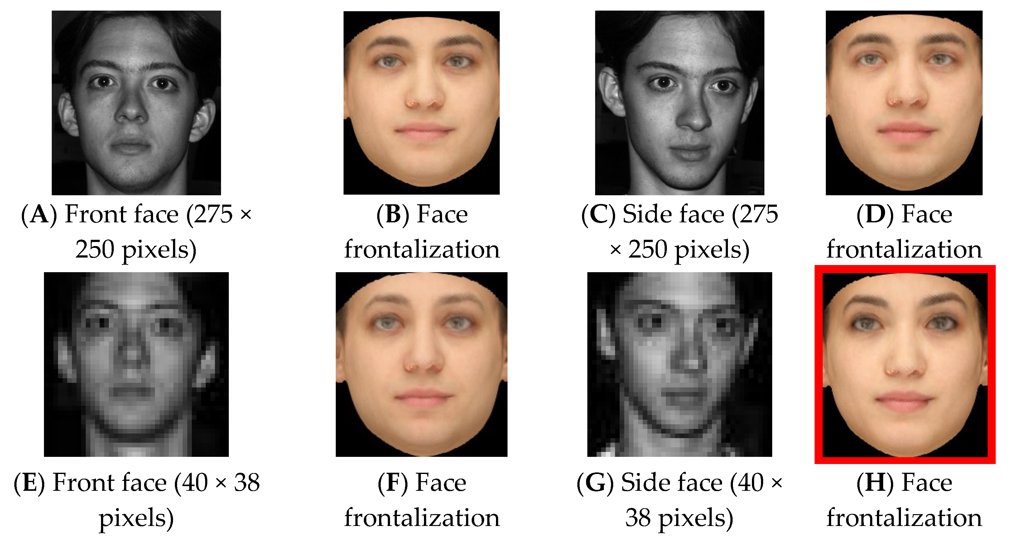
Figure 3.
Training classifiers on the benchmark database.

Figure 4.
Examples of classifier combination.
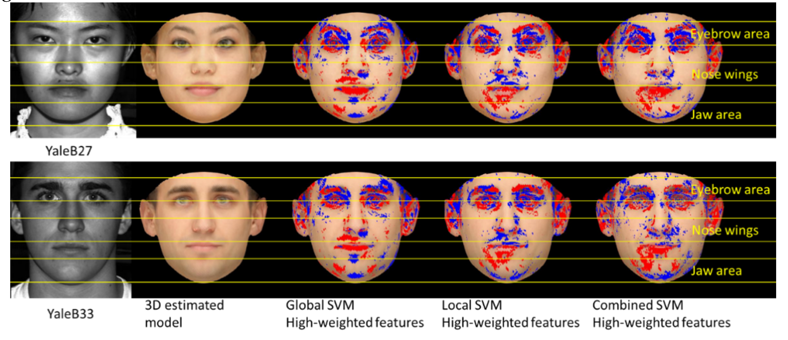
Figure 5.
System structure of our experimental environment.

Figure 6.
People search task processing flowcharts: (a) Wireless sensor network (WSN) node task; and (b) robot process.
Figure 6.
People search task processing flowcharts: (a) Wireless sensor network (WSN) node task; and (b) robot process.
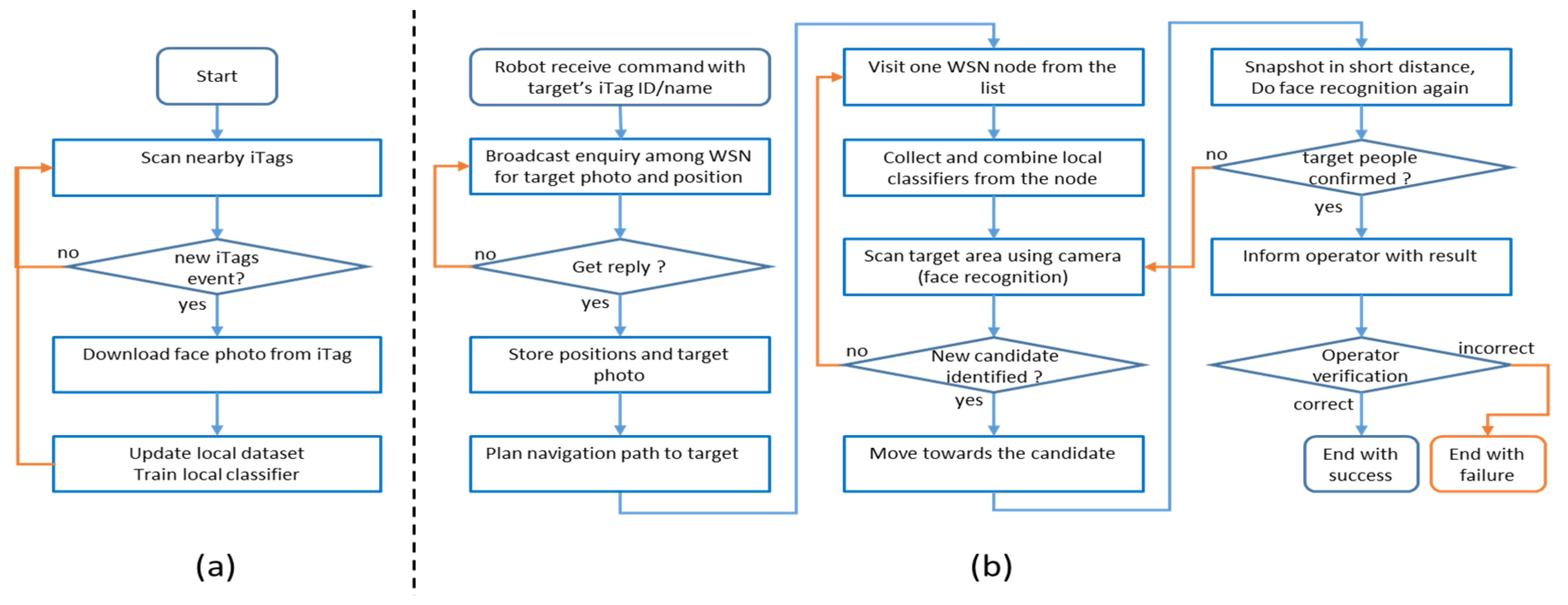
Figure 7.
Real-world experiments. The photos were the actual snapshots taken by the camera mounted on the robot. The low resolution blurred face photos are the targets our method is tackling.
Figure 7.
Real-world experiments. The photos were the actual snapshots taken by the camera mounted on the robot. The low resolution blurred face photos are the targets our method is tackling.


Table 1.
Comparison of recognition rate with global classifiers.
| Photo Size | 240 × 240 | 120 × 120 | 90 × 90 | 60 × 60 | 30 × 30 | 20 × 20 | All |
| Sample number | 756 | 756 | 756 | 756 | 756 | 756 | 756 × 6 |
| Positive samples | 378 | 378 | 378 | 378 | 378 | 378 | 378 × 6 |
| Our method | 93.21% | 91.38% | 91.44% | 90.22% | 88.96% | 83.98% | 89.87% |
| Global SVM | 86.01% | 86.84% | 86.98% | 86.98% | 85.77% | 83.04% | 85.94% |
| Global QDA | 86.90% | 86.77% | 86.51% | 86.38% | 85.19% | 81.22% | 85.49% |
| Global Logistic | 80.56% | 80.56% | 80.82% | 81.35% | 80.56% | 78.44% | 80.38% |
Table 2.
Comparison of false-positive rates with global classifiers.
| Photo Size | 240 × 240 | 120 × 120 | 90 × 90 | 60 × 60 | 30 × 30 | 20 × 20 | All |
| Sample number | 756 | 756 | 756 | 756 | 756 | 756 | 756 × 6 |
| Positive samples | 378 | 378 | 378 | 378 | 378 | 378 | 378 × 6 |
| Our method | 9.27% | 10.56% | 10.43% | 12.21% | 11.73% | 15.16% | 11.56% |
| Global SVM | 20.95% | 20.36% | 20.24% | 20.28% | 21.22% | 22.34% | 20.90% |
| Global QDA | 23.02% | 24.34% | 24.34% | 24.87% | 25.13% | 25.93% | 24.60% |
| Global Logistic | 37.30% | 38.36% | 37.83% | 36.77% | 37.83% | 39.95% | 38.01% |
Table 3.
Comparison of recognition rates with local classifiers.
| Overlapped Data | Photo Size | 240 × 240 | 120 × 120 | 90 × 90 | 60 × 60 | 30 × 30 | 20 × 20 | Average |
|---|---|---|---|---|---|---|---|---|
| 35% | local SVM | 86.64% | 86.77% | 87.63% | 86.26% | 84.02% | 78.24% | 84.93% |
| Our method | 91.27% | 90.34% | 90.34% | 89.02% | 87.70% | 83.86% | 88.76% | |
| 50% | Local SVM | 86.90% | 86.84% | 88.07% | 86.80% | 84.05% | 78.77% | 85.24% |
| Our method | 93.21% | 91.38% | 91.44% | 90.22% | 88.96% | 83.98% | 89.87% | |
| 75% | Local SVM | 87.30% | 87.51% | 88.25% | 86.93% | 84.26% | 79.18% | 85.57% |
| Our method | 92.59% | 89.95% | 90.61% | 88.49% | 88.23% | 82.67% | 88.76% |
Table 4.
Comparison of false positive rates with local classifiers.
| Overlapped Data | Photo Size | 240 × 240 | 120 × 120 | 90 × 90 | 60 × 60 | 30 × 30 | 20 × 20 | Average |
|---|---|---|---|---|---|---|---|---|
| 35% | Local SVM | 13.76% | 14.07% | 12.72% | 14.74% | 13.62% | 15.93% | 14.14% |
| Our method | 10.58% | 11.11% | 11.38% | 12.70% | 13.76% | 15.87% | 12.57% | |
| 50% | Local SVM | 13.49% | 13.99% | 12.41% | 13.76% | 13.60% | 16.72% | 13.99% |
| Our method | 9.27% | 10.56% | 10.43% | 12.21% | 11.73% | 15.16% | 11.56% | |
| 75% | Local SVM | 13.23% | 13.78% | 12.33% | 13.70% | 13.12% | 16.90% | 13.84% |
| Our method | 10.85% | 11.11% | 10.85% | 12.43% | 12.96% | 15.87% | 12.35% |
Table 5.
Comparison between our method and the single pre-trained SVM classifier.
| Classifier | Results | Distance | ||
|---|---|---|---|---|
| Around 3 m | Around 6 m | Around 9 m | ||
| Our method | Number of faces recognized | 49 | 54 | 45 |
| Number of failures (recognition rate) | 5 (89.80%) | 9 (83.33%) | 9 (80.00%) | |
| Single SVM | Number of faces recognized | 62 | 64 | 51 |
| Number of failures (recognition rate) | 10 (83.87%) | 12 (81.25%) | 11 (78.43%) | |
© 2018 by the authors. Licensee MDPI, Basel, Switzerland. This article is an open access article distributed under the terms and conditions of the Creative Commons Attribution (CC BY) license (http://creativecommons.org/licenses/by/4.0/).
Share and Cite
MDPI and ACS Style
Xue, D.; Wang, X.; Zhu, J.; Davis, D.N.; Wang, B.; Zhao, W.; Peng, Y.; Cheng, Y. An Adaptive Ensemble Approach to Ambient Intelligence Assisted People Search. Appl. Syst. Innov. 2018, 1, 33. https://doi.org/10.3390/asi1030033
AMA Style
Xue D, Wang X, Zhu J, Davis DN, Wang B, Zhao W, Peng Y, Cheng Y. An Adaptive Ensemble Approach to Ambient Intelligence Assisted People Search. Applied System Innovation. 2018; 1(3):33. https://doi.org/10.3390/asi1030033
Chicago/Turabian StyleXue, Dongfei, Xiaonian Wang, Jin Zhu, Darryl N. Davis, Bing Wang, Wenbing Zhao, Yonghong Peng, and Yongqiang Cheng. 2018. "An Adaptive Ensemble Approach to Ambient Intelligence Assisted People Search" Applied System Innovation 1, no. 3: 33. https://doi.org/10.3390/asi1030033