New Approximation Methods Based on Fuzzy Transform for Solving SODEs: II


1
Institute of Engineering Mathematics, Universiti Malaysia Perlis, Kampus Tetap Pauh Putra, Arau, Perlis 02600, Malaysia
2
Institute for Research and Applications of Fuzzy Modelling, University of Ostrava, NSC IT4Innovations, 30. Dubna 22, 701 03 Ostrava, Czech Republic
*
Author to whom correspondence should be addressed.
Appl. Syst. Innov. 2018, 1(3), 30; https://doi.org/10.3390/asi1030030
Submission received: 17 June 2018
/
Revised: 11 August 2018
/
Accepted: 14 August 2018
/
Published: 23 August 2018
(This article belongs to the Special Issue Fuzzy Decision Making and Soft Computing Applications)
Abstract
:In this research, three approximation methods are used in the new generalized uniform fuzzy partition to solve the system of differential equations (SODEs) based on fuzzy transform (FzT). New representations of basic functions are proposed based on the new types of a uniform fuzzy partition and a subnormal generating function. The main properties of a new uniform fuzzy partition are examined. Further, the simpler form of the fuzzy transform is given alongside some of its fundamental results. New theorems and lemmas are proved. In accordance with the three conventional numerical methods: Trapezoidal rule (one step) and Adams Moulton method (two and three step modifications), new iterative methods (NIM) based on the fuzzy transform are proposed. These new fuzzy approximation methods yield more accurate results in comparison with the above-mentioned conventional methods.
1. Introduction
Differential equation is particularly useful for different areas of applied sciences and engineering. Many differential equations have no closed form solutions. Thus, many researchers are developing approximation methods for solving differential equations, for example [1,2,3]. In this paper, we continue the study of approximation methods based on FzT to solutions of differential equations.
The core idea of FzT is a fuzzy partition of a universe into fuzzy subsets. The first fuzzy partition of FzT with the Ruspini condition was introduced by [4] and was extensively investigated by [5]. This condition implies normality of the fuzzy partition. In addition, the fuzzy partition with the generalized Ruspini condition (fuzzy r-partition) was introduced by [6]. This fuzzy partition was achieved by replacing the partition of unity by fuzzy r-partition. This type of partition was used by [6,7] for smoothing or filtering data based on the inverse FzT. Further, a generalized fuzzy partition appeared in connection with the notion of the FzT, where FzT components are polynomials of degree m [8]. By [9], different types of fuzzy partitions are taken into consideration such as B-splines, Shepard kernels, Bernstein basis polynomials and Favard-Szasz-Mirakjan operators. Later, the higher degree FzT based on B-splines was proposed [10] to improve the quality of the function approximation of two variables.
A generalized fuzzy partition was implicitly introduced by [11] with the purpose of meeting the requirements of image compression. In addition, a generalized fuzzy partition can also be considered in connection with radial membership functions [12]. Further, necessary and sufficient conditions for modeling the generalized fuzzy partition was provided by [13]. Recently, a new representation formula for basic functions of FzT and a new fuzzy numerical method based on block pulse functions for numerical solution of integral equations were presented by [14]. The approximation method based on the FzT with Shepard-type basic functions for linear Fredholm integral equations was discussed by [15]. New representations of the generalized uniform fuzzy partitions with the normal case to obtain better approximation solutions for solving Cauchy problems were presented by [16].
FzT is a soft computing method developed by Perfilieva [5] that has many applications, for example, in differential and integral equations. FzT for solving ordinary Cauchy problems with one variable was initiated by [4]. The generalization of the Euler method has been discussed by [17] for solving ordinary Cauchy problems. The author has applied this technique to reef growth and sea level variations models. Further, FzT has been generalized from the case of constant components to the case of polynomial components by [8]. Later, the first and second degree FzT based mid-point rule for solving the Cauchy problem and the uncertain initial value problem have been proposed by [18]. Furthermore, an algorithm to obtain the approximate solutions of second order initial value problems was constructed by [19]. From this idea, FzT for numerical solutions of two point boundary value problems was proposed by [20].
FzT of two variables based on finite differences method was used by [21] for solving a type of partial differential equations with Dirichlet boundary conditions and initial conditions. In addition, the first degree FzT of two variables was introduced by [22]. By [23], the partial derivatives using the first FzT were approximated and modification of the Canny edge detector was proposed. Furthermore, the uniform stability result for the vibrations of a telegraph equation using FzT of two variables was proposed by [24]. The composition of inverse and direct discrete FzT method was extended to numerical solution of Fredholm integral equations and Volterra Fredholm integral equations [25]. The general form of the higher order FzT was constructed by [26] for solving differential and integral equations using any arbitrary basis functions. The FzT has investigated for solving the Volterra population growth model using the approximation for the Caputo derivative [27]. A new numerical method based FzT was demonstrated to solve a class of delay differential equations by means of the Picard-like numerical scheme [28]. FzT was considered to approximate the solution of boundary value problems by minimizing the integral squared error in 2-norm [29]. In [30], the dynamical properties of a two neuron system with respect to FzT and a single delay have been investigated. The conditions under which quasi-consensus in a multi-agent system with sampled data based on FzT were proposed by [31].
NIM was proposed to solve nonlinear functional equations and the existence of solution for nonlinear Volterra integral equations [2]. At the same time, NIM was introduced for solving nonlinear equations by using a different decomposition technique [32]. From this conception, NIM was considered in terms up to fourth-order in Taylor series for solving nonlinear equations [33]. Sufficiency conditions have been presented for convergence of the NIM [34]. A new predictor-corrector approach was developed based on NIM for fractional differential equations [35]. Classical methods are modified by [3] to derive numerous formulas for solving the differential equations.
The motivation of the proposed study comes from [16,36,37]. In [16], new fuzzy numerical methods to solve the Cauchy problem was considered and the authors showed that the error can be reduced by FzT and NIM with respect to new generalized uniform fuzzy partitions, namely power of the triangular and raised cosine generalized uniform fuzzy partitions, where generating functions are normal (see also [37] for another approach). In addition, two basic approximation methods, modified Euler method and Trapezoidal rule, with help from FzT for solving SODEs are analyzed in detail by [36]. For this purpose, more generally, new generalized uniform fuzzy partitions are proposed in this study, where a generating function is not normal.
The membership functions in underlying fuzzy partitions are often called basic functions. There has been a growing interest in investigating the properties of fuzzy partitions. However, the problem arises on how one can effectively construct the basic function of fuzzy partitions. In this paper, new representations of basic functions are proposed. This is achieved by introducing new generalized uniform fuzzy partitions, where a generating function is not normal. Further, new fuzzy numerical methods based on NIM and FzT for solving SODEs are introduced and discussed. In particular, we consider functions of two variables with initial conditions. In accordance with the existing methods, Trapezoidal rule and Adams Moulton are improved using FzT and NIM. The methods are combined with one-step, two-step and three-step. As an application, all these methods are used to solve a general model of the dynamical system, i.e., Lotka–Volterra equation with derivatives and with variable coefficients. Furthermore, numerical examples are presented. It is observed that the new fuzzy numerical methods yield more accurate results than classical Trapezoidal rule and classical Adams Moulton methods (2 and 3-step).
The paper is organized as follows. The main part of the paper is Section 3 and Section 4, which provides new representations for basic functions of FzT, followed by the modified one step, 2-step and 3-step based on NIM and FzT method with respect to new representations formulas for generalized uniform fuzzy partition of FzT. In Section 5, numerical examples are discussed. Finally, conclusions are given in Section 6.
2. Basic Concepts
In this section, we give some definitions and introduce the necessary notation following [38], which will be used throughout the paper. Throughout this section, we deal with an interval of real numbers.
Definition 1.
(generalized uniform fuzzy partition) Let be fixed nodes such that , and . We say that the fuzzy sets constitute a generalized fuzzy partition of if the following conditions are fulfilled:
- 1.
- (positivity and locality)— if and if ;
- 2.
- (continuity)— is continuous on ;
- 3.
- (covering)—for .
Fuzzy sets are called basic functions. It is important to remark that by conditions of locality and continuity, . A generalized uniform fuzzy partition of is defined for equidistant nodes, i.e., for all where and two additional properties are satisfied,
- 4.
- for all ;
- 5.
- and for all ;
then the fuzzy partition is called h-uniform generalized fuzzy partition.
Definition 2.
(generating function) A function is called a generating function if it is assumed to be even, continuous and if . The function is even if for all .
The following definition recalls the concept of the generalized fuzzy partition which can be easily extended to the interval . We assume that is partitioned by , according to Definition 1.
Definition 3.
A h-uniform generalized fuzzy partition of interval , determined by the triplet , can be defined using generating function K (Definition 2). Then, basic functions of a h-uniform generalized fuzzy partition are shifted copies of K defined by
for all . The parameter h is called the bandwidth or the shift of the fuzzy partition and the nodes are called the central point of the fuzzy sets .
Remark 1.
A h-uniform fuzzy partition is called Ruspini if the following condition
holds for any . This condition is often called Ruspini condition.
New Iterative Method
NIM have proposed by [2] for solving linear and nonlinear functional equations of the form
where is a known function and N a non linear operator. Solutions obtained by this method are in the form of rapidly converging infinite series which can be effectively approximated by calculating only the first few terms. In this method non linear operator N is decomposed as In [2], the authors were defined the recurrence relation:
Then and . Hence u satisfies the functional (2).
3. New Representations for Basic Functions of FzT
Let us recall the basic facts of an FzT of a continuous real function f as presented by [5,17]. The first step in the definition of the FzT of f involves the selection of a fuzzy partition of the domain by a finite number of fuzzy sets , . In those papers, five axioms specified , , in the fuzzy partition: normality, locality, continuity, unimodality (monotonicity) and orthogonality (Ruspini condition). A fuzzy partition is called uniform if the fuzzy sets , , are shifted copies of symmetrized (more details can be found in [17]). The membership functions , , in a fuzzy partition are called basic functions. Later, a generalized fuzzy partition appeared in connection with the notion of a higher-degree FzT [8]. Furthermore, summarize both these notions in [38]. Three axioms specify , , in the fuzzy partition: positivity and locality, continuity and covering. Recently, the different conditions for generalized uniform fuzzy partitions was proposed [13,38] while another approach was demonstrated by [37] where a function can be reconstructed from its F-transform components. In the following, we modify the definition h-uniform generalized fuzzy partition.
3.1. Generalized Uniform Fuzzy Partitions with the Generalized Normal Case
Let us recall the h-uniform generalized fuzzy partition of real line can be defined using generating function K. Then, basic functions of the h-uniform generalized fuzzy partition are shifted copies of K. On the basis of Definition 1 can be also defined using a generating function where , , and (in general, not necessarily satisfying normal and Ruspini condition) which is that assumed to be even, continuous and if . Therefore, we will modify the basic functions of the h-uniform generalized fuzzy partition so that they are shifted copies of defined by
The parameter h is bandwidth of the fuzzy partition and . The concept of the h-uniform generalized fuzzy partition can be easily extended to the interval as follows.
Definition 4.
Let be fixed nodes within , such that , and . We consider nodes are equidistant, with distance (shift) . A system of fuzzy sets be a generalized uniform fuzzy partitions of if it is defined by
where , , , and . In the sequel, a generating function denote by K and basic functions of FzT denote by .
Lemma 1.
If basic functions of a h-uniform generalized fuzzy partition are shifted copies of defined by (5). Then, .
Proof.
By (5), we get ☐
3.2. Simpler Form of F-Transform Components Based on Generalized Uniform Fuzzy Partitions with the Generalized Normal Case
In this subsection, we present the main principles of FzT with respect to new representations of h-uniform generalized fuzzy partition. Further, we will show that FzT components with respect to new representations of h-uniform generalized fuzzy partition can be simplified and approximated of an original function, say f.
Definition 5.
Let f be a continuous function on and , , be h-uniform generalized fuzzy partition of , . A vector of real numbers given by
for is called the direct FzT of f with respect to .
In the following, we will simplify the representation (6).
Lemma 2.
Let and according to Definition 4, fuzzy sets be a h-uniform generalized fuzzy partition of with a generating function K, then representation (6) of direct FzT can be simplified for as follows
Proof.
By Definition 4, we get
for , , and substituting and then substituting . Thus, we get
and its corresponding results with representation (6). ☐
If , the Lemma 1 still hold by choosing suitable constant , satisfying , where . So, we will restrict ourselves to h-uniform generalized fuzzy partition with , where . In the following, we will simplify the above given expressions for the coefficients in the representation (6). This fact is very important for applications which are more flexible and consequently easier to use.
Corollary 1.
Let the assumptions of Lemma 2 be fulfilled and , where . Then, the coefficients in the expression (6) of the FzT component of f as follows:
for , where interval is partitioned by the h-uniform generalized fuzzy partition .
Proof.
Lemma 3.
Let . Then for any there exist and be basic functions form the h-uniform generalized fuzzy partition of . Let be the integral FzT components of f with respect to . Then for each the following estimations hold: for each and .
Proof.
see [5]. ☐
Corollary 2.
Let the conditions of Lemma 3 be fulfilled. Then for each the following estimations hold: .
The following theorem estimates the difference between the original function and its direct FzT with respect to the h-uniform generalized fuzzy partition.
Theorem 1.
Let and the conditions of Lemma 2 be fulfilled. Then for
where and .
Proof.
By locality condition of definition of h-uniform generalized fuzzy partition, Corollary 1, Lemma 1, and according to [17], using the trapezoid formula with nodes to the numerical computation of the integral, we get for and
Corollary 3.
Let and the conditions of Lemma 2 be fulfilled. Let moreover, f be Lipschitz continuous with respect to t, i.e., there exists a constant , such that for all and ,
Then for
where , , and whenever .
Proof.
By the assumption f has continuous second order derivatives on and is Lipschitz continuous with respect to t. Therefore, using the trapezoid rule and let us choose a value of k in the range and , we get
where , and . ☐
Remark 2.
In view of (13), if . Then,
Definition 6.
Let be direct FzT of a function with respect to the fuzzy partition , of . Then, the function defined on
is called the inverse FzT of f.
The following lemma estimates the difference between the original function and its inverse FzT.
Lemma 4.
Let the assumptions of Theorem 1 and let be the inverse FzT of f with respect to the fuzzy partition of is given by Definition 4. Then, the following estimation holds for and
where and .
Proof.
Let so that for some . By Theorem 1,
Theorem 2.
Let . Thus, for any there exist and be the h-uniform generalized fuzzy partition of defined by (5). Then, the following estimations hold for each .
Proof.
From the proof of Lemma 4 and then using Lemma (3) in the sense that for all ,
Remark 3.
According to Definition (4), it is easy to see that the inverse FzT for all .
On the basis of Definition 4, necessary steps of a new method to construct generalized uniform fuzzy partitions of for solve case K is not normal in the following.
- Select the generating function K which is assumed to be even, continuous and if .
- Specify the value , where to get the normal generating function K and then compute the value , where .
- If conditions holds, then construct generalized uniform fuzzy partitions of by .
Example 1.
Let be defined by
One can see in Table 1 the h-uniform generalized fuzzy partition of determined by Definition 4.
The following remark is for modified Trapezoidal rule based on FzT and NIM to solve SODEs.
Remark 4.
In view of Equation (9), . This means that .
Important property of the direct FzT as well as inverse FzT is their linearity, namely, given and , if , then and .
4. New Fuzzy Numerical Methods for Solving SODEs
Consider the initial value problem (IVP) for the SODEs:
where and f, g are continuous function on . If f (g) satisfies a Lipschitz condition on D in the variable , then the initial-value problem (16) has a unique solution for . In many cases, the problem (16) cannot be solved analytically so that numerical solutions are required. In [16], new representations of basic function based on the FzT are constructed for solving generalized Cauchy problems with help of NIM, FzT and classical methods (one-step, two-step and three-step) have presented while Euler method and Mid-point rule, based on FzT to solve Cauchy problem proposed by [17,18]. Further, NIM has been proposed for solving ODEs and delay differential equations [3]. Moreover, Adams-Bashforth methods and Adams-Moulton methods are noted as two families of multistep methods in literature. Multistep methods refer to using several previous values from the previous steps. The Adams-Bashforth methods were presented by John Couch Adams to solve a differential equation modelling capillary action due to Francis Bashforth and it follows that the Adams-Moulton method was developed improved multistep methods for solving ballistic equations by Forest Ray Moulton. In particular, the Adams-Moulton method is similar to the Adams-Bashforth method and the Adams-Moulton method was used Newton’s method to solve the implicit equation. Clearly, Adams-Bashforth methods are explicit methods and the Adams–Moulton methods are implicit methods, for example, see ([40], p. 111).
Necessary steps of construction of the generalized uniform fuzzy partitions can be summarized as follows.
- Specify the number n of components and compute the step . If we want to obtain as best approximation of f as possible, then n should be large.
- Construct the nodes , where .
- Select the shape of basic functions. This is achieved by selecting the shape of generating function.
- Construct a h-uniform generalized fuzzy partition of by new representations of basic functions are defined by Definition 4.
To begin the derivation of a modified Trapezoidal rule (1-step) and Adams Moulton method (2 and 3-step), integrate (16) on the interval , to obtain=
Consider the following integral
However, we cannot integrate and without knowing and . So, the above integral (18) can be approximated by the following approach
where and are the approximation of f and g on the interval . Choosing different () leads to different schemes. In particular, we choose () which contributes to the one, two and three-step methods based on FzT. Later, modification of these methods based on FzT and NIM.
In this section, we present three new schemes to solve SODEs (16) that use the F-transform and NIM and suppose that the functions f and g on are sufficiently smooth. The first scheme uses 1-step method while the second one uses the 2-step method and the last uses the 3-step method.
4.1. Numerical Scheme I: Modified Trapezoidal Rule Based on FzT and NIM for SODEs
According to necessary steps of construction of the generalized uniform fuzzy partitions in Section 4, we contributed to approximation methods of SODEs (16) by scheme provides formulas for the FzT components, , , of the unknown function with respect to choose some of the h-uniform generalized fuzzy partition, , of interval with parameter h to approximate solution of SODEs (16). As initial step, choose the number and compute , then construct the h-uniform generalized fuzzy partition of using Definition 4. Let . In the following, we apply the FzT and NIM to the SODEs (16) for obtaining the numerical Scheme I, where .
First, let () in the Equation (19) is chosen as
where
and represents the generalized uniform fuzzy partitions that are defined by Definition 4. Then, substituting (20) into (19) for
By Remark 4 in the interval , we have
Hence, the one step method based on FzT for (17) is derived as follows, where .
where and are defined by (21).
This method computes the approximate coordinates and of the FzT for the functions and . The problem with the previous scheme (22) is that the unknown quantities and which means that () appears on both sides and an implicit method. Therefore, one solution to this problem would be to use an explicit method such as another fuzzy approach, namely Scheme I. For this purpose, the scheme (22) is of the form
and can be solved by NIM (2), where
Hence, the three term approximate solution is
and
which leads to the following formulas.
where
In the sequel, the approximate solution of SODEs (16) can be obtained using the inverse FzT as follows:
4.2. Numerical Scheme II: Modified 2-Step Adams Moulton Method Based on FzT and NIM for SODEs
The Scheme I uses 1-step method for solving SODEs (16). In this subsection, we improve 2-step Adams Moulton method using FzT and NIM for solving SODEs (16). Let us recall that the modified 2-step Adams Moulton method proposed by [16]. From this idea, the modified 2-step Adams Moulton method can be extended to approximate the solution of (16) by necessary steps of construction of the generalized uniform fuzzy partitions in Section 4. It is worth noting that three terms of NIM were used in [16], while four terms of NIM are used in this study. Let FzT components, , , of the unknown function with respect to choose some of the h-uniform generalized fuzzy partition (5) and let , and if possible; otherwise, we can compute FzT components from the numerical Scheme I. In the following, we apply the F-transform and NIM to the SODEs (16) for obtaining the numerical Scheme II, where . First, if in the Equation (19) is approximated by
where
. Substituting (26) into (19), then for
Similarity,
The problem with the previous scheme (27) is that the unknown quantities and . Therefore, one solution to this problem would be to use an explicit method. For this purpose, the scheme (27) is of the form
and can be solved by NIM (2), where
Hence, the four term approximate solution is
and
which leads to the following formulas.
where
Then, obtain the desired approximation for by the inverse FzT (25) applied to and .
4.3. Numerical Scheme III: Modified 3-Step Adams Moulton Method Based on FzT and NIM for SODEs
In this subsection, we improve 3-step Adams Moulton method using FzT and NIM for solving SODEs (16). The modified 3-step Adams Moulton method proposed by [16] for solving Cauchy problems. From this idea, we can propose to approximate the solution of (16) by NIM and FzT components, , , of the unknown function with respect to choose some of the h-uniform generalized fuzzy partition (see Definition 4), , of interval with parameter , . Let if possible; otherwise, we can compute FzT components from the numerical Scheme I. Now, we apply the F -transform and NIM to the SODEs (16) and obtain the following numerical Scheme III for :
According to steps of deriving Equation (27) and then steps of NIM in previous SubSection 4.2, we get the four term approximation of the NIM as follows.
Hence, the four term approximate solution is
and
which leads to the following formulas.
where
4.4. Error Analysis of Numerical Scheme I for SODEs
In this subsection, we present error analysis for numerical Scheme I and consider the Formula (23). If denote the exact solution and denote the numerical solution. Then, substituting the exact solution in the Formula (23), we get
where
and the truncation error of the scheme I are given by
Rearranging (23), we get
Similarly to Lemma 8 and Theorem 2 by [16], we have the following results.
Lemma 5.
Let are assumed to be sufficiently smooth functions of its arguments on and be Lipschitz continuous with respect to x and y, i.e., there exists a constant , such that for all and ,
Assume that , is a h-uniform generalized fuzzy partition of . Then we get for ,
where , , are determined by Formula (31) and are upper bound for f and g respectively on .
Theorem 3.
Let be twice continuously differentiable on . Let moreover, be Lipschitz continuous with respect to x and y. Assume that , is a h-uniform generalized fuzzy partition of . Then the scheme I (23) is convergent.
The technique of error analysis for rest schemes can be obtained analogously to numerical Scheme I.
5. Applications
A general model for the dynamical system may be written as , where g and h are arbitrary functions of the prey and predator species whose populations are and at time t. However, the following problem of Lotka–Volterra equation with derivatives and with variable coefficients as functions of time t have not yet been solved by any fuzzy numerical method. The new differential equations are represented by a non-autonomous ordinary differential equation system. The model, incorporating the above functions is as follows [41,42,43]:
Two examples are discussed in order to prove that the results obtained by Scheme I (23), II (28) and III (29) for the numerical solution of the model (36).
Example 2.
Consider the problem of Lotka-Volterra-prey- predator model (36). We take .
Example 3.
Consider the problem of Lotka-Volterra-prey-predator model (36) with .
The results are listed in Table 2, Table 3, Table 4, Table 5 and Table 6 by the proposed fuzzy approximation methods with respect to case is defined by Example 1. The proposed fuzzy approximation methods are generated by Algorithms Algorithm A1, Algorithm A2 and Algorithm A3 (Appendix A). The mean square error (MSE) defined as . This is an easily computable quantity for a particular sample. From the numerical tests, the results are summarized as follows:
- Moreover, comparison of MSE for Examples 2 and 3 shown in Table 6. It is observed that the new fuzzy approximation methods yield more accurate results in comparison with the classical Trapezoidal rule (one step) and classical Adams Moulton method (two and three steps). Hence, the new fuzzy approximation methods provide alternative techniques for solving SODEs with better results.
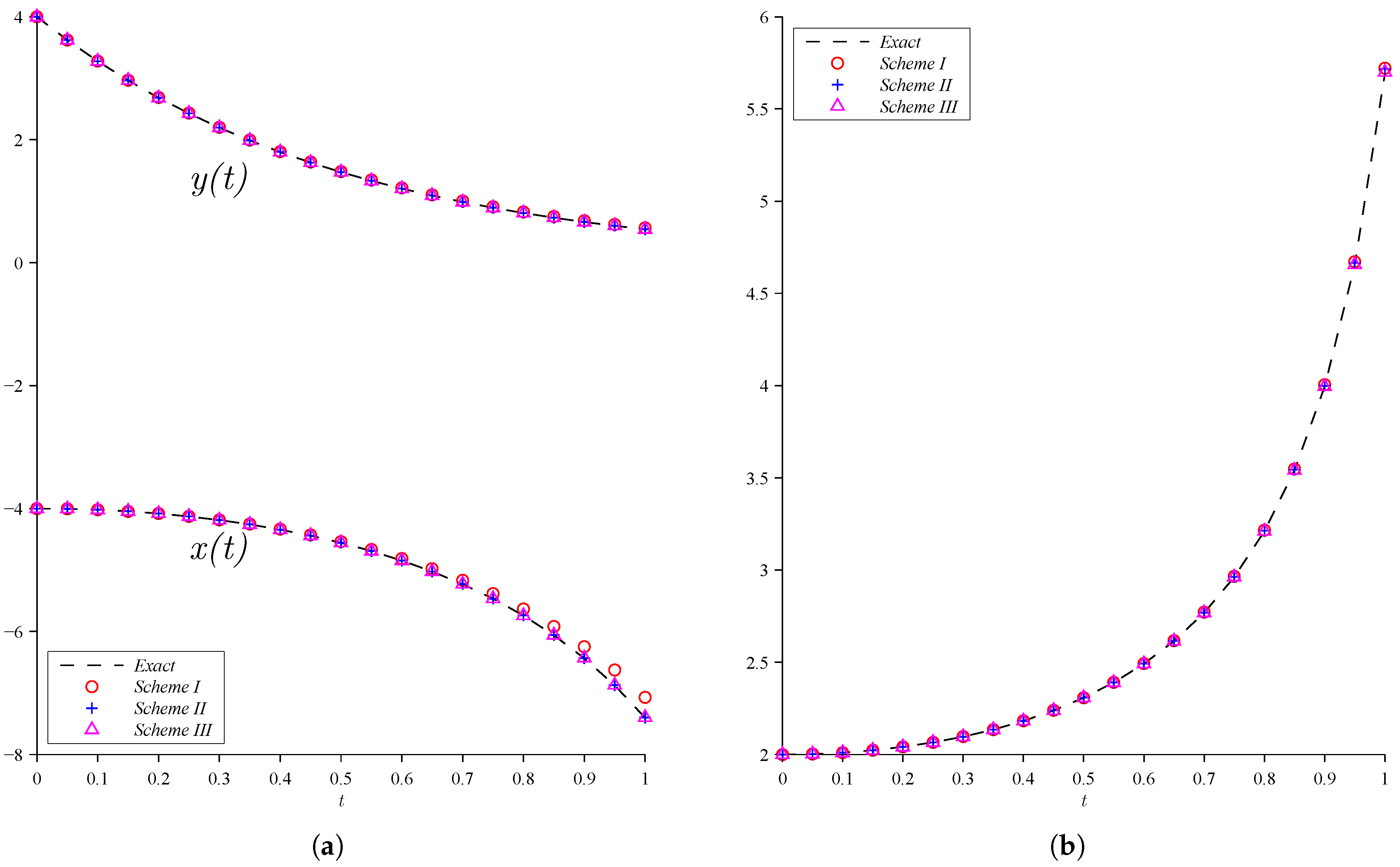
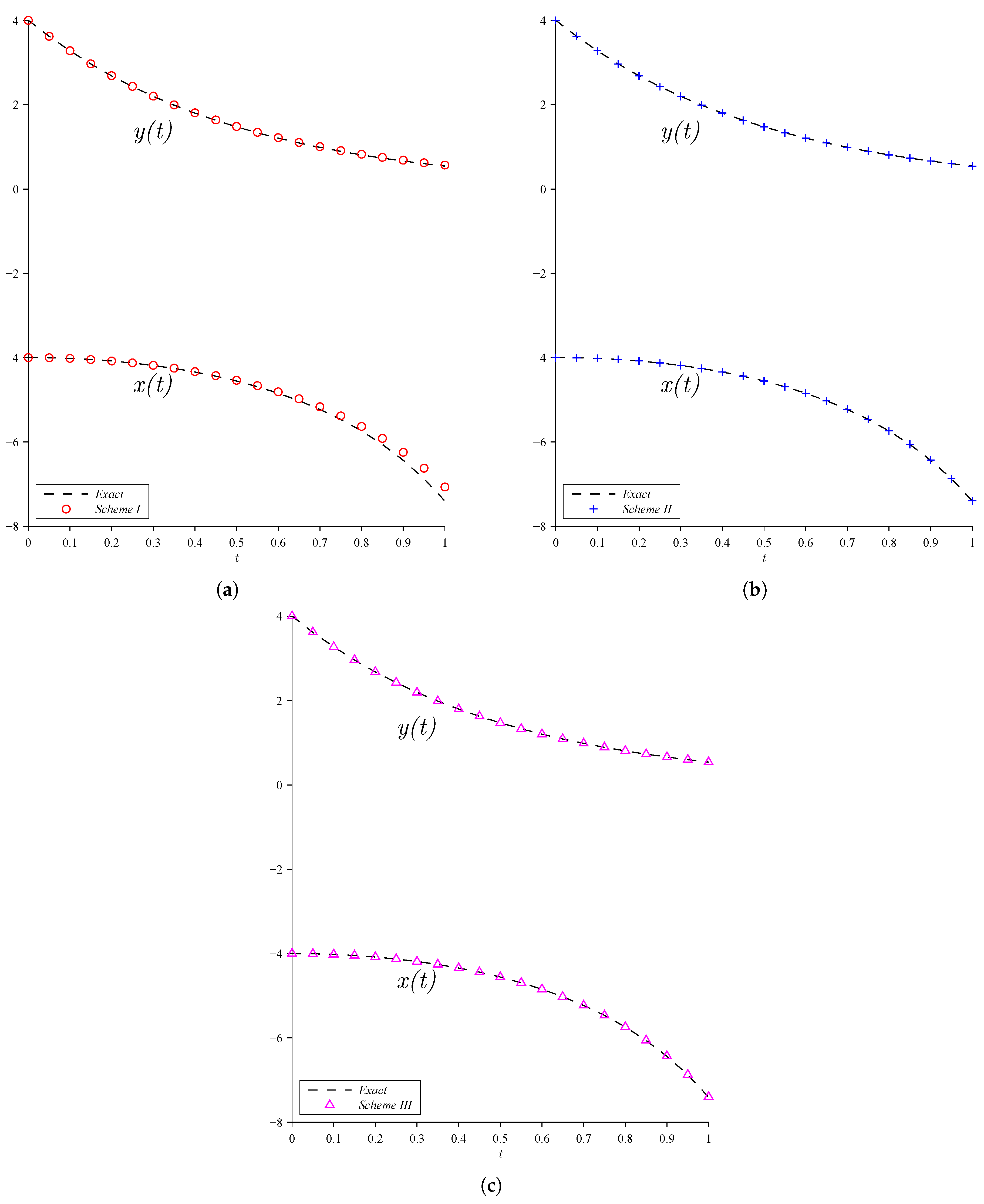
Further, the results obtained using proposed fuzzy approximation methods for Examples 2 and 3 are shown in Figure 1, Figure 2 and Figure 3 by using . In view of Figure 2 and Figure 3, the graphical results of Examples 2 and 3 show a comparison between numerical Schemes (I, II and III) and exact solutions are shown separated from each other for clarity while a comparison between three proposed fuzzy numerical methods (Schemes I, II and III) and exact solution are shown in Figure 1. Furthermore, in view of Figure 2 and Figure 3, a comparison between the numerical results and exact solutions for . All the graphs are plotted using MATLAB software.
6. Conclusions
Three approximation methods are used the new generalized uniform fuzzy partitions for solving SODEs. In accordance with the three approximation methods for Cauchy problem by [16], Trapezoidal rule (one step) and Adams Moulton method (two and three steps) are improved using FzT and NIM. The results proved that the first approximation method converged to the exact solution. As an application, a predator-prey model is solved by using three proposed approximation methods. From the numerical results, it is observed that the new fuzzy approximation methods yield more accurate results in comparison with the classical Trapezoidal rule (one step) and classical Adams Moulton method (two and three steps). So, it is recommended to use the proposed methods to solve differential equations.
In this regard, it is well-known that FzT has a certain advantage to cope with problems affected by noise. This is because the FzT components of original and noisy functions are very similar to each other. In addition, we can reduce a higher-order differential equation into a system of first-order differential equations by relabeling the variables. Thus, the proposed methods can also be applied to a higher-order differential equation in the case of non-noisy or noisy right-hand side. From Algorithms Algorithm A1, Algorithm A2and Algorithm A3 (Appendix A), it is observed that the new fuzzy approximation methods are more time consuming in comparison with the considered Trapezoidal rule and the Adams Moulton methods. In the future research, we plan to give more details about running time of proposed methods. Further, we plan to solve a boundary value problem for a second order ordinary differential equation with fuzzy boundary conditions, see preliminary results in [44].
Author Contributions
Conceptualization and performed the numerical experiments, H.A.A.; Evaluated the results and supported this work, I.P.; Project administration and designed the numerical methods, M.Z.A.; Software and data curation, Z.R.Y.
Funding
This work of Irina Perfilieva has been supported by the project “LQ1602 IT4Innovations excellence in science” and by the Grant Agency of the Czech Republic (project No. 16-09541S).
Acknowledgments
The authors would like to express their deep gratitude to the editors and the anonymous referees for their valuable comments and criticism towards the improvement of the paper. Also, many thanks given to Universiti Malaysia Perlis for providing all facilities until this work was completed successfully.
Conflicts of Interest
The authors declare no conflicts of interest.
Appendix A. Algorithms
In this appendix, algorithms of approximation methods based on FzT and NIM for Section 4.1, Section 4.2 and Section 4.3 are explained with details. A pseudocode is used to describe the algorithms and simplified code that is easy to read. This pseudocode specifies the form of the input to be supplied and the form of the desired output. As a consequence, a stopping technique independent of the numerical technique is incorporated into each algorithm to avoid infinite loops. Two punctuation symbols are used in the algorithms, a period (.) indicates the termination of a step and a semicolon (;) separates tasks within a step. In algorithms with help of MATLAB software, the definite integral is specified by integral (function, upper limits, lower limits). The steps in the algorithms follow the rules of structured program construction. They have been arranged so that there should be minimal difficulty translating pseudocode into any programming language suitable for scientific applications. To approximate the solution of SODEs (16) at () equally spaced numbers in the interval , proceed as follows.

Algorithm A1.
One-step algorithm for system of ODEs.
| INPUT: ; ; endpoints ; integer N; initial condition ; m. |
| Step 1 Set ; ; ; ; ; . |
| Step 2 Define the generalized uniform fuzzy partitions as . |
| Step 3 for to N do Steps 04–15. |
| end. |
| OUTPUT: Approximation X and Y to x and y, respectively at the () values of t. |
Algorithm A2.
Two-step algorithm for system of ODEs.
| INPUT: ; ; endpoints ; integer N; initial condition ; m. |
| Step 1 Set ; ; ; ; ; . |
| Step 2 Define the generalized uniform fuzzy partitions as . |
| Step 3 Set ; . (In the case of no exact solutions, compute and using Algorithm 1.) |
| Step 4 for to N do Steps 05–18. |
| end. |
| OUTPUT: Approximation X and Y to x and y, respectively at the () values of t. |
Algorithm A3.
Three-step algorithm for system of ODEs.
| INPUT: ; ; endpoints ; integer N; initial condition ; m. |
| Step 1 Set ; ; ; ; ; . |
| Step 2 Define the generalized uniform fuzzy partitions as . |
| Step 3 Set ; ; ; . (In the case of no exact solutions, compute , , and using Algorithm 1 or 2.) |
| Step 4 for to N do Steps 05–20. |
| end. |
| OUTPUT: Approximation X and Y to x and y, respectively at the () values of t. |
References
- Ahmad, M.Z.; Hasan, M.K.; Baets, B.D. Analytical and numerical solutions of fuzzy differential equations. Inf. Sci. 2013, 236, 156–167. [Google Scholar] [CrossRef]
- Daftardar-Gejji, V.; Jafari, H. An iterative method for solving nonlinear functional equations. J. Math. Anal. Appl. 2006, 316, 753–763. [Google Scholar] [CrossRef]
- Sukale, Y.; Daftardar-Gejji, V. New Numerical Methods for Solving Differential Equations. Int. J. Appl. Comput. Math. 2017, 3, 1639–1660. [Google Scholar] [CrossRef]
- Perfilieva, I.; Haldeeva, E. Fuzzy transformation. In Proceedings of the Joint 9th IFSA World Congress and 20th NAFIPS International Conference, Vancouver, BC, Canada, 25–28 July 2001; Volume 4, pp. 1946–1948. [Google Scholar]
- Perfilieva, I. Fuzzy transforms: Theory and applications. Fuzzy Sets Syst. 2006, 157, 993–1023. [Google Scholar] [CrossRef]
- Stefanini, L. F-transform with parametric generalized fuzzy partitions. Fuzzy Sets Syst. 2011, 180, 98–120. [Google Scholar] [CrossRef]
- Holčapek, M.; Tichý, T. A smoothing filter based on fuzzy transform. Fuzzy Sets Syst. 2011, 180, 69–97. [Google Scholar] [CrossRef] [Green Version]
- Perfilieva, I.; Daňková, M.; Bede, B. Towards a higher degree F-transform. Fuzzy Sets Syst. 2011, 180, 3–19. [Google Scholar] [CrossRef]
- Bede, B.; Rudas, I.J. Approximation properties of fuzzy transforms. Fuzzy Sets Syst. 2011, 180, 20–40. [Google Scholar] [CrossRef]
- Kokainis, M.; Asmuss, S. Higher Degree F-transforms Based on B-splines of Two Variables. In Information Processing and Management of Uncertainty in Knowledge-Based Systems; Carvalho, J.P., Lesot, M.J., Kaymak, U., Vieira, S., Bouchon-Meunier, B., Yager, R.R., Eds.; Springer International Publishing: Cham, Switzerland, 2016; pp. 648–659. [Google Scholar]
- Hurtik, P.; Perfilieva, I. Image Compression Methodology Based on Fuzzy Transform. In International Joint Conference CISIS’12-ICEUTE’12-SOCO’12 Special Sessions; Springer: Berlin/Heidelberg, Germany, 2013; pp. 525–532. [Google Scholar]
- Patané, G. Fuzzy transform and least-squares approximation: Analogies, differences, and generalizations. Fuzzy Sets Syst. 2011, 180, 41–54. [Google Scholar] [CrossRef]
- Holčapek, M.; Perfilieva, I.; Novák, V.; Kreinovich, V. Necessary and sufficient conditions for generalized uniform fuzzy partitions. Fuzzy Sets Syst. 2015, 277, 97–121. [Google Scholar] [CrossRef] [Green Version]
- Khastan, A. A new representation for inverse fuzzy transform and its application. Soft Comput. 2017, 21, 3503–3512. [Google Scholar] [CrossRef]
- Ziari, S.; Perfilieva, I. On the approximation properties of fuzzy transform. J. Intell. Fuzzy Syst. 2017, 33, 171–180. [Google Scholar] [CrossRef]
- Alkasasbeh, H.A.; Perfilieva, I.; Ahmad, M.Z.; Yahya, Z.R. New fuzzy numerical methods for solving Cauchy problems. Appl. Syst. Innov. 2018, 1, 15. [Google Scholar] [CrossRef]
- Perfilieva, I. Fuzzy transform: Application to the Reef growth problem. In Fuzzy Logic in Geology; Demicco, R.V., Klir, G.J., Eds.; Academic Press: Amsterdam, The Netherlands, 2003; Chapter 9; pp. 275–300. [Google Scholar]
- Khastan, A.; Perfilieva, I.; Alijani, Z. A new fuzzy approximation method to Cauchy problems by fuzzy transform. Fuzzy Sets Syst. 2016, 288, 75–95. [Google Scholar] [CrossRef]
- Chen, W.; Shen, Y. Approximate solution for a class of second-order ordinary differential equations by the fuzzy transform. J. Intell. Fuzzy Syst. 2014, 27, 73–82. [Google Scholar]
- Alireza, K.; Zahra, A.; Irina, P. Fuzzy transform to approximate solution of two-point boundary value problems. Math. Meth. Appl. Sci. 2017, 40, 6147–6154. [Google Scholar]
- Holcapek, M.; Valášek, R. Numerical solution of partial differential equations with the help of fuzzy transform technique. In Proceedings of the 2017 IEEE International Conference on Fuzzy Systems (FUZZ-IEEE), Naples, Italy, 9–12 July 2017; pp. 1–6. [Google Scholar]
- Hodáková, P.; Perfilieva, I. F1-transform of Functions of Two Variables. In EUSFLAT 2013; Atlantis Press: Milan, Italy, 2013; pp. 547–553. [Google Scholar]
- Perfilieva, I.; Hodáková, P.; Hurtík, P. Differentiation by the F-transform and application to edge detection. Fuzzy Sets Syst. 2016, 288, 96–114. [Google Scholar] [CrossRef]
- Ghosh, R.; Chowdhury, S.; Gorain, G.C.; Kar, S. Uniform stabilization of the telegraph equation with a support by fuzzy transform method. QSci. Connect 2014, 2014, 19. [Google Scholar] [CrossRef]
- Ezzati, R.; Mokhtari, F.; Maghasedi, M. Numerical solution of Volterra-Fredholm integral equations with the help of inverse and direct discrete fuzzy transforms and collocation technique. Int. J. Ind. Math. 2012, 4, 221–229. [Google Scholar]
- Zeinali, M.; Alikhani, R.; Shahmorad, S.; Bahrami, F.; Perfilieva, I. On the structural properties of Fm-transform with applications. Fuzzy Sets Syst. 2018, 342, 32–52. [Google Scholar] [CrossRef]
- Baleanu, D.; Agheli, B.; Adabitabar Firozja, M.; Al Qurashi, M.M. A method for solving nonlinear Volterra’s population growth model of noninteger order. Adv. Differ. Equ. 2017, 2017, 368. [Google Scholar] [CrossRef]
- Tomasiello, S. An alternative use of fuzzy transform with application to a class of delay differential equations. Int. J. Comput. Math. 2017, 94, 1719–1726. [Google Scholar] [CrossRef]
- Alijani, Z.; Khastan, A.; Khattri, S.K.; Tomasiello, S. Fuzzy Transform to Approximate Solution of Boundary Value Problems via Optimal Coefficients. In Proceedings of the 2017 International Conference on High Performance Computing Simulation (HPCS), Genoa, Italy, 17–21 July 2017; pp. 466–471. [Google Scholar]
- Tomasiello, S. A First Investigation on the Dynamics of Two Delayed Neurons through Fuzzy Transform Approximation. In Proceedings of the 2017 International Conference on High Performance Computing Simulation (HPCS), Genoa, Italy, 17–21 July 2017; pp. 460–465. [Google Scholar]
- Tomasiello, S.; Gaeta, M.; Loia, V. Quasi–consensus in Second–Order Multi–agent Systems with Sampled Data Through Fuzzy Transform. J. Uncertain Syst. 2016, 10, 243–250. [Google Scholar]
- Noor, M.A.; Noor, K.I.; Mohyud-Din, S.T.; Shabbir, A. An iterative method with cubic convergence for nonlinear equations. Appl. Math. Comput. 2006, 183, 1249–1255. [Google Scholar] [CrossRef]
- Saeed, R.K.; Aziz, K.M. An iterative method with quartic convergence for solving nonlinear equations. Appl. Math. Comput. 2008, 202, 435–440. [Google Scholar] [CrossRef]
- Bhalekar, S.; Daftardar-Gejji, V. Convergence of the New Iterative Method. Int. J. Differ. Equ. 2011, 2011, 10. [Google Scholar] [CrossRef]
- Daftardar-Gejji, V.; Sukale, Y.; Bhalekar, S. A new predictor-corrector method for fractional differential equations. Appl. Math. Comput. 2014, 244, 158–182. [Google Scholar] [CrossRef]
- Alkasasbeh, H.A.; Perfilieva, I.; Ahmad, M.Z.; Yahya, Z.R. New approximation methods based on fuzzy transform for solving SODEs: I. Appl. Syst. Innov. 2018, 1, 29. [Google Scholar]
- Perfilieva, I.; Holčapek, M.; Kreinovich, V. A new reconstruction from the F-transform components. Fuzzy Sets Syst. 2016, 288, 3–25. [Google Scholar] [CrossRef]
- Perfilieva, I. F-Transform. In Handbook of Computational Intelligence; Kacprzyk, J., Pedrycz, W., Eds.; Springer: Berlin/Heidelberg, Germany, 2015; Chapter 7; pp. 113–130. [Google Scholar]
- Jahedi, S.; Mehdipour, M.; Rafizadeh, R. Approximation of integrable function based on ø-transform. Soft Comput. 2013, 18, 2015–2022. [Google Scholar] [CrossRef]
- Butcher, J.C. Numerical Methods for Ordinary Differential Equations, 3rd ed.; John Wiley & Sons, Ltd.: Hoboken, NJ, USA, 2016. [Google Scholar]
- Bougoffa, L. Solvability of the predator and prey system with variable coefficients and comparison of the results with modified decomposition. Appl. Math. Comput. 2006, 182, 383–387. [Google Scholar] [CrossRef]
- Yusufoğlu, E.; Erbaş, B. He’s variational iteration method applied to the solution of the prey and predator problem with variable coefficients. Phys. Lett. A 2008, 372, 3829–3835. [Google Scholar] [CrossRef]
- González-Parra, G.C.; Arenas, A.J.; Cogollo, M.R. Numerical-analytical solutions of predator-prey models. WSEAS Trans. Biol. Biomed. 2013, 10, 79–87. [Google Scholar]
- Hodakova, P.; Perfilieva, I.; Valasek, R. A new approach to fuzzy boundary value problem. In Uncertainty Modelling in Knowledge Engineering and Decision Making; World Scientific Proceedings Series on Computer Engineering and Information Science; World Scientific: Singapore, 2016; pp. 276–281. [Google Scholar]
Figure 1.
A comparison between three fuzzy numerical methods and exact solution for two examples. (a) Example 2; (b) Example 3.
Figure 1.
A comparison between three fuzzy numerical methods and exact solution for two examples. (a) Example 2; (b) Example 3.

Figure 2.
The graphical solution of Example 2. (a) Scheme I; (b) Scheme II; (c) Scheme III.

Figure 3.
The graphical solution of Example 3. (a) Scheme I; (b) Scheme II; (c) Scheme III.
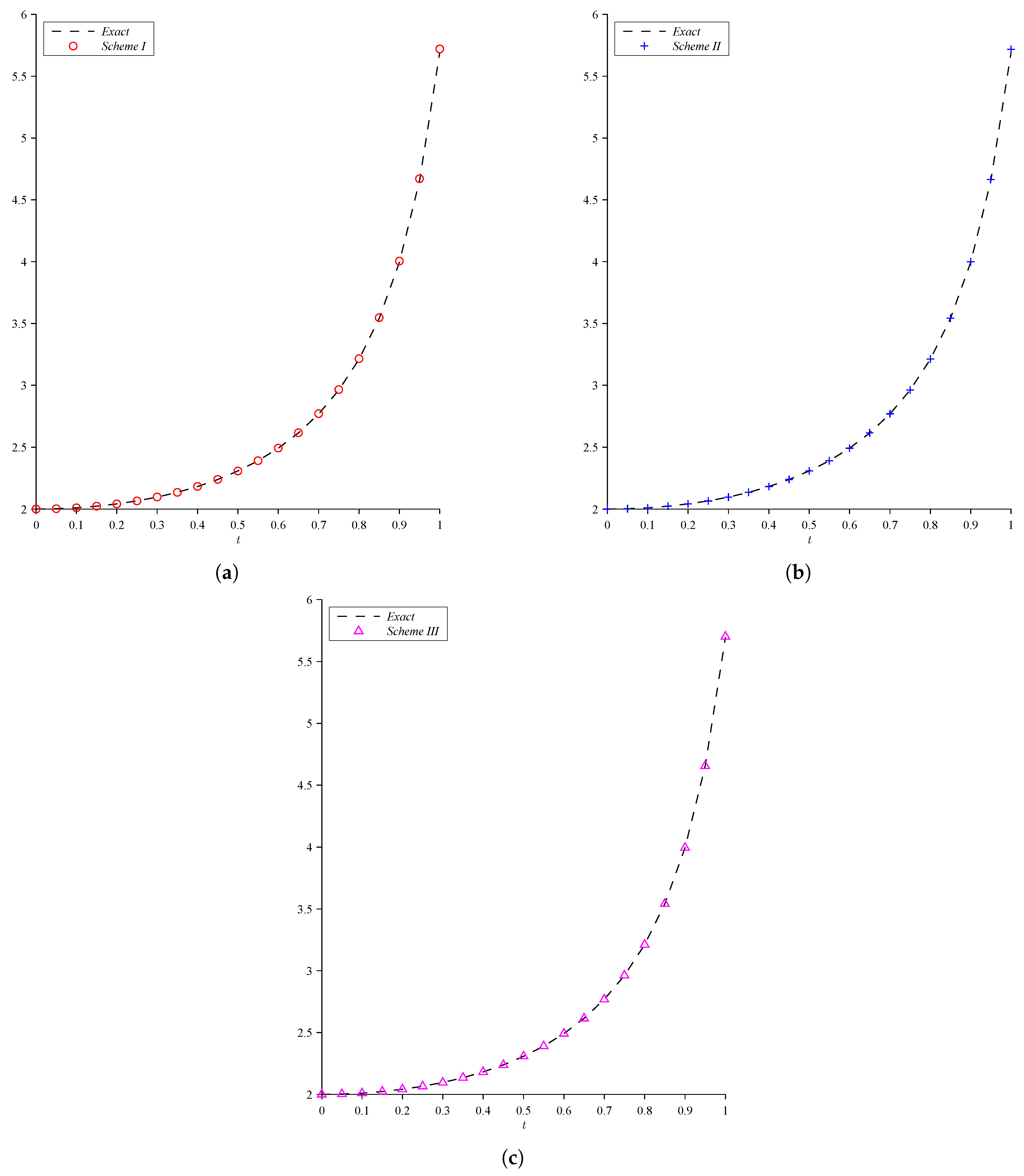
Table 1.
Example 1.
Table 2.
Comparison of numerical results of for Example 2.
| Solution | Proposed Scheme I | Proposed Scheme II | Proposed Scheme III | Trap | 2-Step Adams | 3-Step Adams | |
|---|---|---|---|---|---|---|---|
| 0.00 | −4.00000 | −4.00000 | −4.00000 | −4.00000 | −4.00000 | −4.00000 | −4.00000 |
| 0.05 | −4.00501 | −4.00506 | −4.00501 | −4.00501 | −4.00714 | −4.00501 | −4.00501 |
| 0.10 | −4.02008 | −4.02059 | −4.02011 | −4.02008 | −4.02627 | −4.02187 | −4.02008 |
| 0.15 | −4.04543 | −4.04589 | −4.04536 | −4.04536 | −4.05752 | −4.04875 | −4.04703 |
| 0.20 | −4.08136 | −4.08128 | −4.08121 | −4.08119 | −4.10134 | −4.08610 | −4.08434 |
| 0.25 | −4.12834 | −4.12721 | −4.12813 | −4.12811 | −4.15850 | −4.13442 | −4.13261 |
| 0.30 | −4.18701 | −4.18423 | −4.18673 | −4.18670 | −4.23015 | −4.19440 | −4.19250 |
| 0.35 | −4.25816 | −4.25304 | −4.25783 | −4.25779 | −4.31783 | −4.26691 | −4.26487 |
| 0.40 | −4.34282 | −4.33453 | −4.34243 | −4.34236 | −4.42361 | −4.35300 | −4.35077 |
| 0.45 | −4.44224 | −4.42976 | −4.44178 | −4.44170 | −4.55014 | −4.45399 | −4.45151 |
| 0.50 | −4.55798 | −4.54001 | −4.55745 | −4.55733 | −4.70086 | −4.57151 | −4.56871 |
| 0.55 | −4.69195 | −4.66686 | −4.69134 | −4.69117 | −4.88023 | −4.70755 | −4.70433 |
| 0.60 | −4.84651 | −4.81220 | −4.84581 | −4.84558 | −5.09399 | −4.86455 | −4.86079 |
| 0.65 | −5.02460 | −4.97833 | −5.02378 | −5.02346 | −5.34964 | −5.04556 | −5.04112 |
| 0.70 | −5.22984 | −5.16805 | −5.22887 | −5.22845 | −5.65700 | −5.25435 | −5.24903 |
| 0.75 | −5.46680 | −5.38480 | −5.46565 | −5.46508 | −6.02912 | −5.49569 | −5.48924 |
| 0.80 | −5.74130 | −5.63286 | −5.73990 | −5.73914 | −6.48349 | −5.77559 | −5.76768 |
| 0.85 | −6.06076 | −5.91759 | −6.05906 | −6.05803 | −7.04390 | −6.10182 | −6.09202 |
| 0.90 | −6.43490 | −6.24582 | −6.43281 | −6.43141 | −7.74310 | −6.48450 | −6.47222 |
| 0.95 | −6.87660 | −6.62636 | −6.87400 | −6.87209 | −8.62699 | −6.93706 | −6.92148 |
| 1.00 | −7.40326 | −7.07221 | −7.40106 | −7.39831 | −9.76103 | −7.47766 | −7.45769 |
Trapezoidal rule; 2-Step Adams Moulton Method; 3-Step Adams Moulton Method.
Table 3.
Comparison of numerical results of for Example 2.
| Solution | Proposed Scheme I | Proposed Scheme II | Proposed Scheme III | Trap | 2-Step Adams | 3-Step Adams | |
|---|---|---|---|---|---|---|---|
| 0.00 | 4.00000 | 4.00000 | 4.00000 | 4.00000 | 4.00000 | 4.00000 | 4.00000 |
| 0.05 | 3.61935 | 3.62135 | 3.61935 | 3.61935 | 3.62045 | 3.61935 | 3.61935 |
| 0.10 | 3.27492 | 3.27848 | 3.27485 | 3.27492 | 3.27766 | 3.27601 | 3.27492 |
| 0.15 | 2.96327 | 2.96802 | 2.96314 | 2.96327 | 2.96757 | 2.96496 | 2.96415 |
| 0.20 | 2.68128 | 2.68698 | 2.68112 | 2.68124 | 2.68671 | 2.68326 | 2.68261 |
| 0.25 | 2.42612 | 2.43262 | 2.42595 | 2.42607 | 2.43201 | 2.42819 | 2.42769 |
| 0.30 | 2.19525 | 2.20247 | 2.19508 | 2.19520 | 2.20079 | 2.19724 | 2.19688 |
| 0.35 | 1.98634 | 1.99425 | 1.98619 | 1.98630 | 1.99067 | 1.98815 | 1.98792 |
| 0.40 | 1.79732 | 1.80593 | 1.79718 | 1.79729 | 1.79951 | 1.79888 | 1.79875 |
| 0.45 | 1.62628 | 1.63564 | 1.62616 | 1.62627 | 1.62541 | 1.62754 | 1.62752 |
| 0.50 | 1.47152 | 1.48170 | 1.47143 | 1.47153 | 1.46664 | 1.47245 | 1.47253 |
| 0.55 | 1.33148 | 1.34257 | 1.33142 | 1.33153 | 1.32166 | 1.33207 | 1.33224 |
| 0.60 | 1.20478 | 1.21688 | 1.20474 | 1.20485 | 1.18908 | 1.20500 | 1.20526 |
| 0.65 | 1.09013 | 1.10337 | 1.09012 | 1.09023 | 1.06762 | 1.08998 | 1.09033 |
| 0.70 | 0.98639 | 1.00091 | 0.98641 | 0.98652 | 0.95615 | 0.98587 | 0.98632 |
| 0.75 | 0.89252 | 0.90848 | 0.89257 | 0.89269 | 0.85366 | 0.89163 | 0.89217 |
| 0.80 | 0.80759 | 0.82515 | 0.80766 | 0.80779 | 0.75923 | 0.80632 | 0.80696 |
| 0.85 | 0.73073 | 0.75011 | 0.73084 | 0.73097 | 0.67208 | 0.72910 | 0.72984 |
| 0.90 | 0.66120 | 0.68260 | 0.66133 | 0.66148 | 0.59150 | 0.65919 | 0.66004 |
| 0.95 | 0.59827 | 0.62195 | 0.59844 | 0.59860 | 0.51692 | 0.59590 | 0.59686 |
| 1.00 | 0.54134 | 0.56745 | 0.54145 | 0.54163 | 0.44787 | 0.53860 | 0.53969 |
Trapezoidal rule; 2-Step Adams Moulton Method; 3-Step Adams Moulton Method.
Table 4.
Comparison of numerical results of for Example 3.
| Solution | Proposed Scheme I | Proposed Scheme II | Proposed Scheme III | Trap | 2-Step Adams | 3-Step Adams | |
|---|---|---|---|---|---|---|---|
| 0.00 | 2.00000 | 2.00000 | 2.00000 | 2.00000 | 2.00000 | 2.00000 | 2.00000 |
| 0.05 | 2.00250 | 2.00257 | 2.00250 | 2.00250 | 2.00250 | 2.00250 | 2.00250 |
| 0.10 | 2.01008 | 2.01016 | 2.01007 | 2.01008 | 2.01005 | 2.01006 | 2.01008 |
| 0.15 | 2.02289 | 2.02299 | 2.02289 | 2.02289 | 2.02279 | 2.02285 | 2.02286 |
| 0.20 | 2.04124 | 2.04138 | 2.04124 | 2.04124 | 2.04101 | 2.04117 | 2.04118 |
| 0.25 | 2.06557 | 2.06577 | 2.06558 | 2.06558 | 2.06511 | 2.06546 | 2.06547 |
| 0.30 | 2.09650 | 2.09676 | 2.09652 | 2.09651 | 2.09567 | 2.09633 | 2.09633 |
| 0.35 | 2.13485 | 2.13520 | 2.13488 | 2.13486 | 2.13344 | 2.13459 | 2.13459 |
| 0.40 | 2.18171 | 2.18218 | 2.18176 | 2.18172 | 2.17942 | 2.18132 | 2.18132 |
| 0.45 | 2.23852 | 2.23915 | 2.23860 | 2.23854 | 2.23493 | 2.23795 | 2.23796 |
| 0.50 | 2.30720 | 2.30803 | 2.30731 | 2.30722 | 2.30167 | 2.30637 | 2.30638 |
| 0.55 | 2.39031 | 2.39140 | 2.39047 | 2.39034 | 2.38192 | 2.38910 | 2.38911 |
| 0.60 | 2.49133 | 2.49279 | 2.49157 | 2.49138 | 2.47868 | 2.48956 | 2.48957 |
| 0.65 | 2.61513 | 2.61708 | 2.61549 | 2.61520 | 2.59605 | 2.61251 | 2.61251 |
| 0.70 | 2.76863 | 2.77126 | 2.76917 | 2.76873 | 2.73967 | 2.76465 | 2.76466 |
| 0.75 | 2.96202 | 2.96563 | 2.96288 | 2.96218 | 2.91754 | 2.95585 | 2.95584 |
| 0.80 | 3.21093 | 3.21600 | 3.21235 | 3.21120 | 3.14130 | 3.20103 | 3.20099 |
| 0.85 | 3.54059 | 3.54791 | 3.54308 | 3.54108 | 3.42845 | 3.52398 | 3.52386 |
| 0.90 | 3.99443 | 4.00539 | 3.99914 | 3.99541 | 3.80653 | 3.96482 | 3.96449 |
| 0.95 | 4.65413 | 4.67130 | 4.66407 | 4.65640 | 4.32100 | 4.59671 | 4.59578 |
| 1.00 | 5.69348 | 5.72071 | 5.71719 | 5.69904 | 5.05197 | 5.56751 | 5.56473 |
Trapezoidal rule; 2-Step Adams Moulton Method; 3-Step Adams Moulton Method.
Table 5.
Comparison of numerical results of for Example 3.
| Solution | Proposed Scheme I | Proposed Scheme II | Proposed Scheme III | Trap 1 | 2-Step Adams 2 | 3-Step Adams 3 | |
|---|---|---|---|---|---|---|---|
| 0.00 | 2.00000 | 2.00000 | 2.00000 | 2.00000 | 2.00000 | 2.00000 | 2.00000 |
| 0.05 | 2.00250 | 2.00257 | 2.00250 | 2.00250 | 2.00250 | 2.00250 | 2.00250 |
| 0.10 | 2.01008 | 2.01016 | 2.01007 | 2.01008 | 2.01005 | 2.01006 | 2.01008 |
| 0.15 | 2.02289 | 2.02299 | 2.02289 | 2.02289 | 2.02279 | 2.02285 | 2.02286 |
| 0.20 | 2.04124 | 2.04138 | 2.04124 | 2.04124 | 2.04101 | 2.04117 | 2.04118 |
| 0.25 | 2.06557 | 2.06577 | 2.06558 | 2.06558 | 2.06511 | 2.06546 | 2.06547 |
| 0.30 | 2.09650 | 2.09676 | 2.09652 | 2.09651 | 2.09567 | 2.09633 | 2.09633 |
| 0.35 | 2.13485 | 2.13520 | 2.13488 | 2.13486 | 2.13344 | 2.13459 | 2.13459 |
| 0.40 | 2.18171 | 2.18218 | 2.18176 | 2.18172 | 2.17942 | 2.18132 | 2.18132 |
| 0.45 | 2.23852 | 2.23915 | 2.23860 | 2.23854 | 2.23493 | 2.23795 | 2.23796 |
| 0.50 | 2.30720 | 2.30803 | 2.30731 | 2.30722 | 2.30167 | 2.30637 | 2.30638 |
| 0.55 | 2.39031 | 2.39140 | 2.39047 | 2.39034 | 2.38192 | 2.38910 | 2.38911 |
| 0.60 | 2.49133 | 2.49279 | 2.49157 | 2.49138 | 2.47868 | 2.48956 | 2.48957 |
| 0.65 | 2.61513 | 2.61708 | 2.61549 | 2.61520 | 2.59605 | 2.61251 | 2.61251 |
| 0.70 | 2.76863 | 2.77126 | 2.76917 | 2.76873 | 2.73967 | 2.76465 | 2.76466 |
| 0.75 | 2.96202 | 2.96563 | 2.96288 | 2.96218 | 2.91754 | 2.95585 | 2.95584 |
| 0.80 | 3.21093 | 3.21600 | 3.21235 | 3.21120 | 3.14130 | 3.20103 | 3.20099 |
| 0.85 | 3.54059 | 3.54791 | 3.54308 | 3.54108 | 3.42845 | 3.52398 | 3.52386 |
| 0.90 | 3.99443 | 4.00539 | 3.99914 | 3.99541 | 3.80653 | 3.96482 | 3.96449 |
| 0.95 | 4.65413 | 4.67130 | 4.66407 | 4.65640 | 4.32100 | 4.59671 | 4.59578 |
| 1.00 | 5.69348 | 5.72071 | 5.71719 | 5.69904 | 5.05197 | 5.56751 | 5.56473 |
Trapezoidal rule; 2-Step Adams Moulton Method; 3-Step Adams Moulton Method.
Table 6.
The values of MSE for Examples 2 and 3.
| (a) The Values of MSE offor SODEs | |||||||
| Case | Proposed Scheme for | Classical Method for | |||||
| I | II | III | Trapezoidal Rule | 2-Step Adams Moulton | 3-Step Adams Moulton | ||
| Ex.1 | 1.21569 × | 1.21112 × | 3.71739 × | 5.99915 × | 8.37463 × | 4.72086 × | |
| Ex.2 | 6.02153 × | 3.29699 × | 1.77640 × | 2.75574 × | 9.75470 × | 1.01541 × | |
| (b) The Values of MSE of for SODEs | |||||||
| Case | Proposed Scheme for | Classical Method for | |||||
| I | II | III | Trapezoidal Rule | 2-Step Adams Moulton | 3-Step Adams Moulton | ||
| Ex.1 | 1.80417 × | 1.20902 × | 2.08739 × | 1.40165 × | 2.25155 × | 1.09674 × | |
| Ex.2 | 6.02153 × | 3.29699 × | 1.77640 × | 2.75574 × | 9.75470 × | 1.01541 × | |
© 2018 by the authors. Licensee MDPI, Basel, Switzerland. This article is an open access article distributed under the terms and conditions of the Creative Commons Attribution (CC BY) license (http://creativecommons.org/licenses/by/4.0/).
Share and Cite
MDPI and ACS Style
ALKasasbeh, H.; Perfilieva, I.; Ahmad, M.Z.; Yahya, Z.R. New Approximation Methods Based on Fuzzy Transform for Solving SODEs: II. Appl. Syst. Innov. 2018, 1, 30. https://doi.org/10.3390/asi1030030
AMA Style
ALKasasbeh H, Perfilieva I, Ahmad MZ, Yahya ZR. New Approximation Methods Based on Fuzzy Transform for Solving SODEs: II. Applied System Innovation. 2018; 1(3):30. https://doi.org/10.3390/asi1030030
Chicago/Turabian StyleALKasasbeh, Hussein, Irina Perfilieva, Muhammad Zaini Ahmad, and Zainor Ridzuan Yahya. 2018. "New Approximation Methods Based on Fuzzy Transform for Solving SODEs: II" Applied System Innovation 1, no. 3: 30. https://doi.org/10.3390/asi1030030