Prediction of Temperature Distribution in Orthogonal Machining Based on the Mechanics of the Cutting Process Using a Constitutive Model

Abstract

This paper presents an original method of predicting temperature distribution in orthogonal machining based on a constitutive model of various materials and the mechanics of their cutting process. Currently, temperature distribution is commonly investigated using arduous experiments, computationally inefficient numerical analyses, and complex analytical models. In the method proposed herein, the average temperatures at the primary shear zone (PSZ) and the secondary shear zone (SSZ) were determined for various materials, based on a constitutive model and a chip-formation model using measurements of cutting force and chip thickness. The temperatures were determined when differences between predicted shear stresses using the Johnson–Cook constitutive model (J–C model) and those using a chip-formation model were minimal. J–C model constants from split Hopkinson pressure bar (SHPB) tests were adopted from the literature. Cutting conditions, experimental cutting force, and chip thickness were used to predict the shear stresses. The temperature predictions were compared to documented results in the literature for AISI 1045 steel and Al 6082-T6 aluminum in multiple tests in an effort to validate this methodology. Good agreement was observed for the tests with each material. Thanks to the reliable and easily measurable cutting forces and chip thicknesses, and the simple forms of the employed models, the presented methodology has less experimental complexity, less mathematical complexity, and high computational efficiency.

1. Introduction

Determination of the temperature distribution is needed in the machining process because of its controlling influence on tool performance, and the quality of the machined part. Elevated temperatures have a negative impact on tool performance due to the softening of tool materials, and increasing diffusion, which also affect the quality of the machined part. It is well known that the increasing temperature in machining is caused by large plastic deformation. The shear plane heat source at the primary shear zone (PSZ) and the frictional heat source at the tool–chip interface (secondary shear zone, SSZ) are the two principal heat sources in machining. However, an accurate and convenient method for determining temperature distribution remains challenging due to the complexity of the contact condition, and the restricted accessibility during the cutting process.

Previous researchers made considerable progress in determining temperature distribution in machining. Experimental approaches, numerical approaches, and analytical approaches were developed in the past.

Experimental approaches using tool–work thermocouples, embedded thermocouples, radiation pyrometers, metallographic techniques, and a method using fine powders with a constant melting point were reported for measuring the temperatures of tools and workpieces. The tool–work-thermocouple technique was applied in milling and turning experiments with various metallic materials [1,2,3]. In this method, the contact area between the tool and the workpiece forms a hot junction, while the remote sections of the tool and the workpiece form a cold junction, and the average temperature at the SSZ is measured experimentally. The embedded-thermocouple technique was utilized to measure the temperature distribution of cutting tools. The thermocouple is inserted into a machined hole inside the cutting tool with varying depths [4,5]. Radiation techniques were applied using an infrared (IR) pyrometer or an IR camera to measure the surface temperatures of the workpieces and the cutting tools, based on their emitted thermal energy [6,7,8,9]. The metallographic technique was utilized to investigate temperature by correlating the temperature with changes in microstructure and hardness due to elevated temperatures [10]. The fine-powder method was also used to find the temperature distribution within tools by observing the boundary line formed by melted powder scattered on the tool’s surface [11]. The experimental approaches are arduous and difficult to implement in machining tests due to the complex contact phenomena and the restricted accessibility, especially in high-speed machining.

Numerical approaches were developed based on finite-element (FE) simulations for modeling orthogonal machining processes. Dawson et al. predicted the shear plane temperature using a FE solution for the heat-transfer problem with an assumption of a moving band heat source [12]. Kim et al. developed a thermo-viscoplastic cutting model using a finite-element method (FEM) to analyze the mechanics of the steady-state orthogonal cutting process. The temperature distribution was analyzed in this model by removing spurious oscillations which occurred in the solution [13]. Moriwaki et al. developed a rigid-plastic FE model in orthogonal cutting, and the temperature distributions in workpieces and tools were analyzed based on the stress, strain, and material flow in the workpiece [14]. Lei et al. developed a thermomechanical plane-strain FE model for the orthogonal cutting process with continuous chip formation [15]. Levy et al. applied a two-dimensional finite-difference approach to determine the transient temperature variation in chips and cutting tools in orthogonal cutting [16]. Chan et al. developed a thermal analysis using the boundary element method for the metal cutting process [17]. Umbrello et al. developed a FE model to predict temperature when steady-state conditions were reached. The heat transfer coefficient between tools and workpieces in steady-state conditions was determined using a pure thermal simulation. The determined coefficient was then used in a thermomechanical simulation for temperature prediction [18]. Kim et al. and Yang et al. developed similar FE models to investigate the temperature field in laser-assisted machining [19,20]. Özel et al. developed a FE model to investigate the influence of cutting-tool edge roundness on the temperature field at tool–chip and tool–work interfaces [21]. Attia et al. developed a FE model to investigate the influence of tool coatings on the temperature field [22]. Although numerical approaches using FEM made considerable progress in predicting temperature distribution in machining, the high computational cost and the large number of input parameters, including contact conditions, and material properties of cutting tools and workpieces, which must be obtained from extensive experimental work and material property tests, cause inconvenience and difficulty in the temperature prediction. Chip morphology, cutting force, temperature distribution, and residual stress obtained from experiments are needed for comparison with the simulation results for calibration and validation.

Analytical approaches were developed to predict temperature distribution in machining. Boothroyd developed an analytical model for temperature prediction using Wiener’s energy partition analysis [23,24]. The following assumptions were made in this model: (1) independent workpiece thermal properties; (2) uniform heat sources on the tool rake face; (3) a constant fraction of total heat transferred into the tool; and (4) negligible heat transfer in the chip flow direction. Radulescu et al. developed an analytical model to calculate transient cutting temperature using cutting forces as inputs. The heat fluxes in the tools, chips, and workpieces were determined from the energy balance in the controlled volume of the chip formation area [25]. In order to reduce computing time and to simplify input requirements, Stephenson et al. developed a similar approach using insulated boundary conditions to predict transient temperature [26]. Komanduri et al. developed a temperature prediction model that combined the effects of the shear plane heat source at the PSZ and the frictional heat source at the SSZ [27]. The temperature increases in the chip and in the workpiece due to the heat source in the PSZ were solved using a modification of Hahn’s moving oblique band heat source model [28]. The temperature increase due to the heat source in the SSZ was solved using a modified Jaeger’s moving band heat source model in the chip, and a stationary rectangular heat source model in the tool [29]. Liang et al. further developed this model to predict temperature distribution with considerations of the tool thermal properties and the tool wear effects [30,31]. Liang et al. also developed a cutting temperature model with an assumption of non-uniform heat intensity and partition ratio, and reported improved accuracy upon validation [32]. Korkut et al. employed regression analysis and neural network analysis to predict the temperature of the tool–chip interface [33]. The abovementioned analytical models have high mathematical complexity, which reduces the computational efficiency.

In this work, the authors present an original method of predicting temperature distribution in machining, specifically the average temperatures at the PSZ and at the SSZ, using a J–C model and a chip formation model. Experimental measurements of cutting forces and chip thicknesses, cutting conditions, and J–C model constants were used as inputs. The cutting conditions, and the reliable and easily measurable cutting forces and chip thicknesses were adopted from the literature, in which simple orthogonal cutting tests were conducted. The simple form of the J–C model, and the simple calculations in the chip formation model reduced the mathematical complexity and the computational cost of the proposed method. The J–C model constants are readily available for common metal materials in machining such as steels, aluminum alloys, and titanium alloys. Therefore, the proposed methodology has the advantages of less experimental complexity, less mathematical complexity, and high computational efficiency.

1.1. Johnson–Cook Constitutive Model

Constitutive relationships describe material behavior under various mechanical and thermal loading conditions. The J–C model is one of the most widely used constitutive relationships for the analytical modeling of force, temperature, and residual stress in machining because it is effective, simple, and easy to use. The J–C model is a semi-empirical constitutive model that predicts the flow stress of materials at high strains, high strain rates, and elevated temperatures. The J–C model can be expressed as the following equation:

$$\sigma =\left(A+B{\epsilon }^n\right)\left(1+C\ln \left(\frac{\dot{\epsilon }}{\dot{{\epsilon }_0}}\right)\right)\left(1-{\left(\frac{T- T_r}{T_m- T_r}\right)}^m\right),$$

(1)

where A, B, C, m, and n are five materials constants. A is the yield strength, B is the strength coefficient, C is the strain rate coefficient, n is the strain hardening coefficient, and m is the thermal softening coefficient. $\sigma$ is the flow stress, $\epsilon$ is the plastic strain, $\dot{\epsilon }$ is the plastic strain rate, $\dot{{\epsilon }_0}$ is the reference plastic strain rate, T is the temperature of the workpiece material, $T_r$ is the reference temperature, and $T_m$ is the melting temperature of the material.

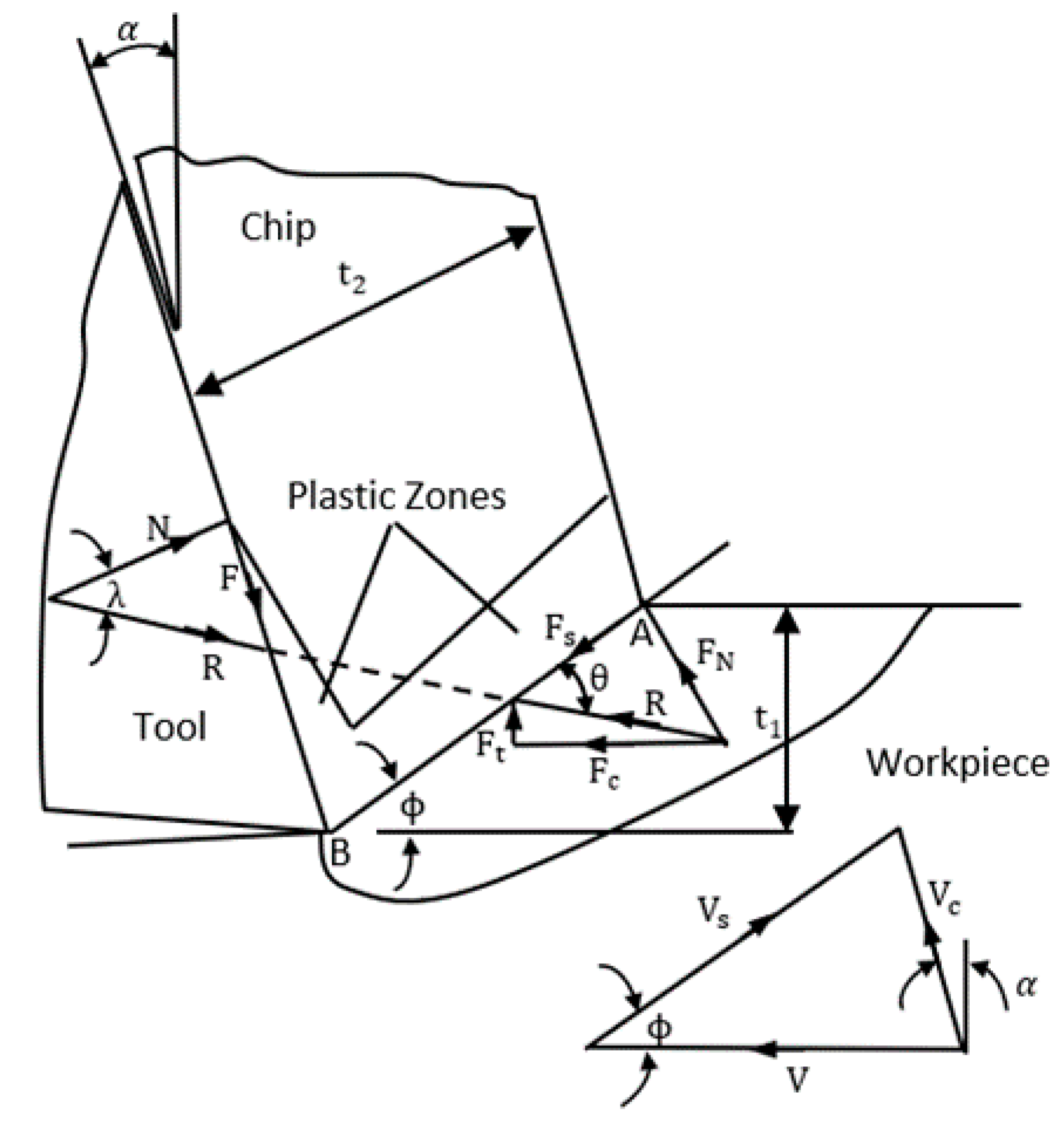
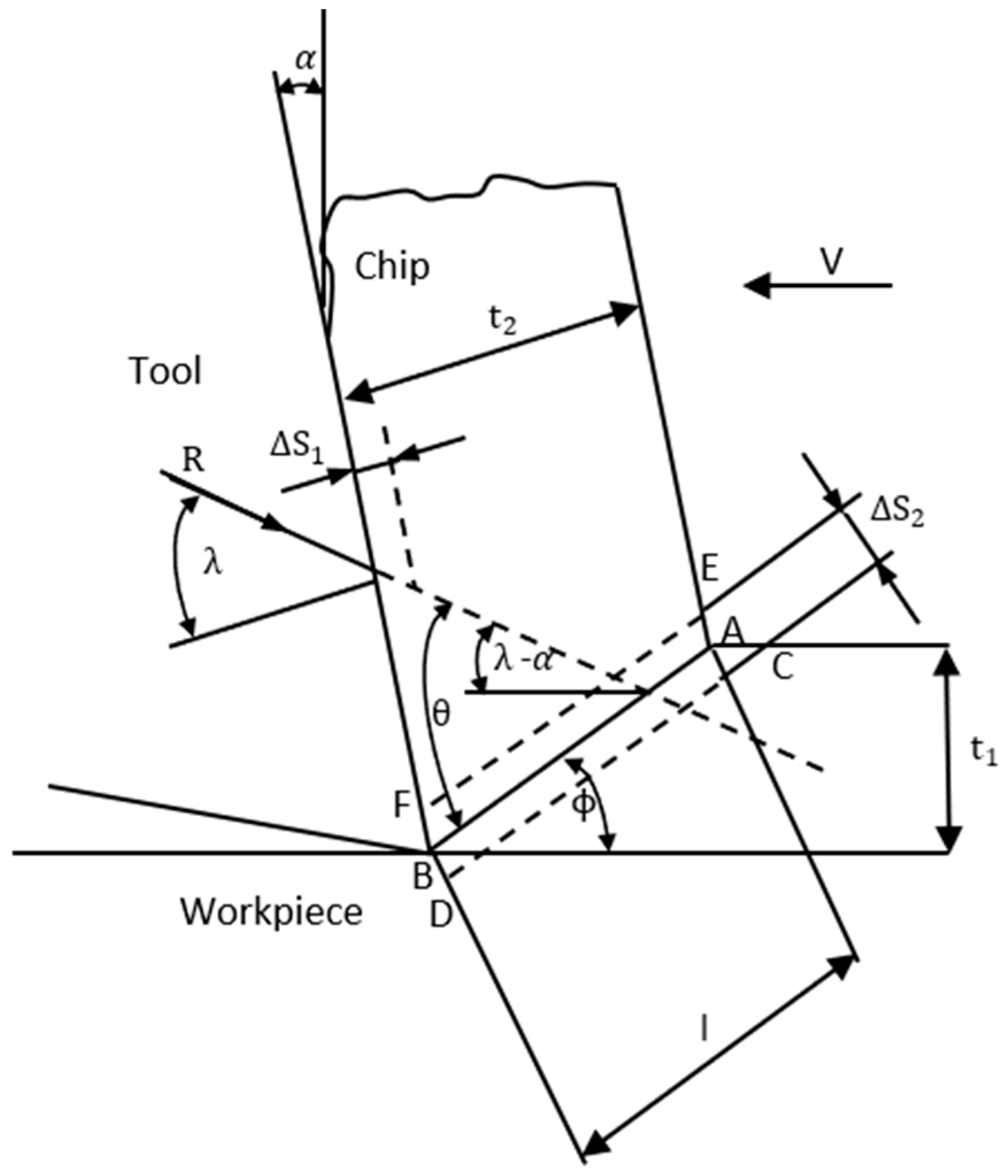
1.2. Chip Formation Model

The chip formation model, as originally proposed by Oxley [34], based on orthogonal cutting, is widely used in the predictions of machining force, temperature, and residual stress with the available properties of workpiece materials, and cutting conditions. The chip formation model is illustrated in Figure 1, where α is the rake angle, ϕ is the shear angle, λ is average friction angle at the tool–chip interface, and θ is the angle between the resultant cutting force (R) and the primary shear zone (AB). t₁ and t₂ are the depth of the cut, and the chip thickness, respectively. $V, V_s,\mathrm{and}{V}_c$ are the cutting velocity, the shear velocity, and the chip velocity respectively. w is the cutting width, which is not shown in Figure 1. The assumptions made in the chip formation model are a perfectly sharp cutting tool, plain strain, steady-state conditions, a straight-line shape of shear zones, and uniform stress and temperature at shear zones. The PSZ and SSZ are characterized as the region encompassing line AB, and the region encompassing the tool–chip interface, respectively, as illustrated in Figure 2. Strain rate constants ($C_0 \mathrm{and}\delta$) are defined as the ratio of the shear plane length to the thickness of the PSZ (l/Δs₂), and the ratio of the thickness of the SSZ to the chip thickness (Δs₁/t₂), respectively.

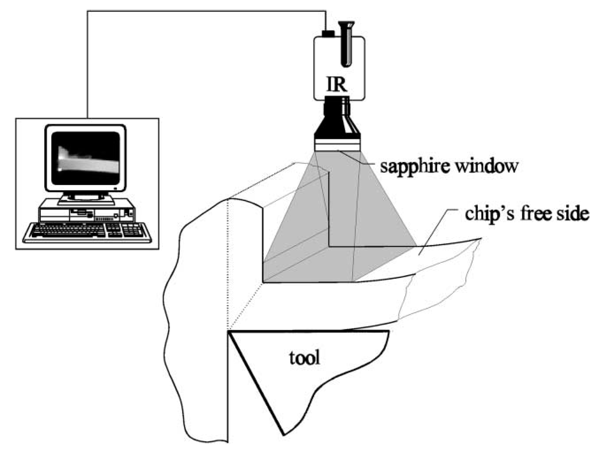
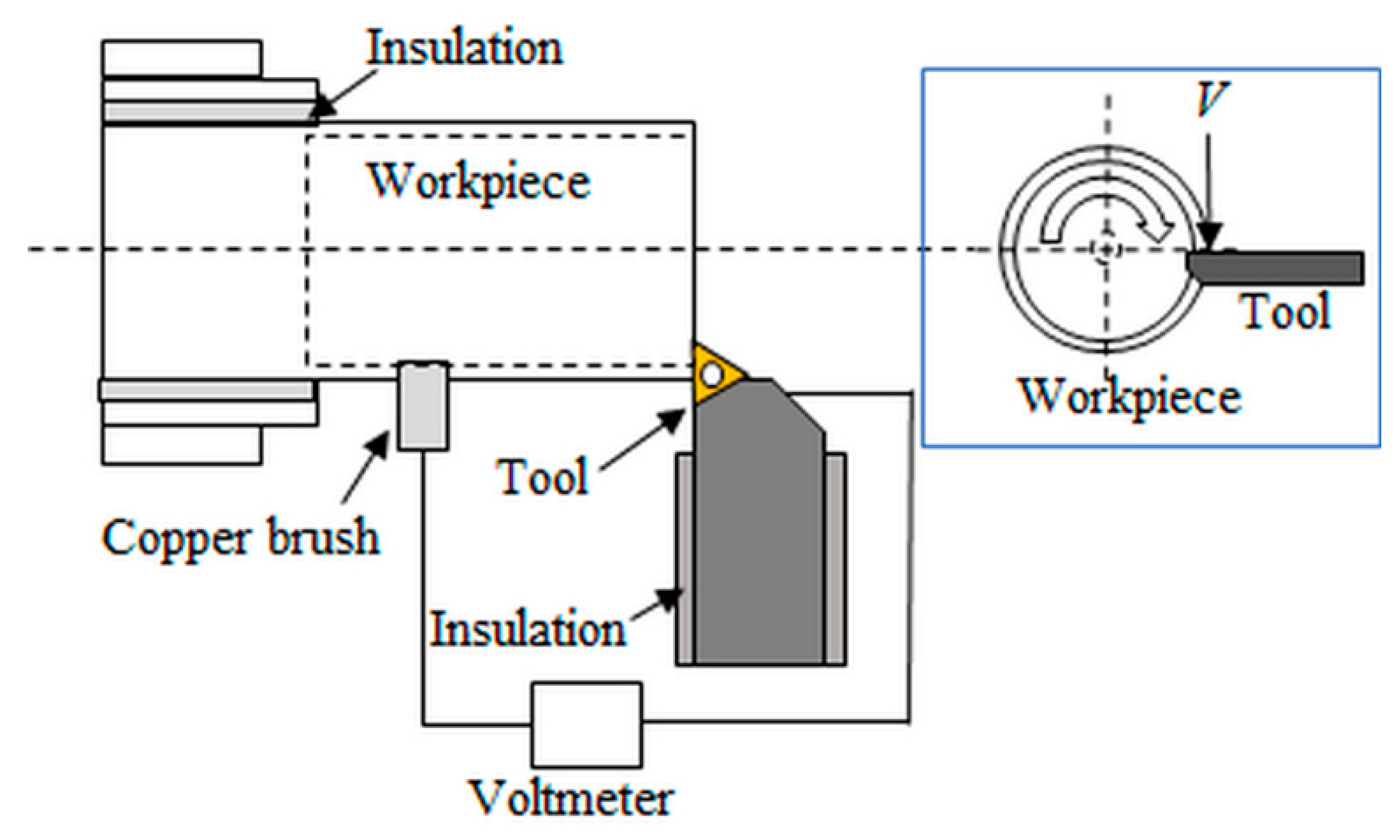
1.3. Experimental Measurements

The experimental data used in this paper were adopted from previous works found in the literature [36,37]. The experimental forces were measured using a piezoelectric dynamometer in three mutually perpendicular directions. The cutting force and thrust force were then obtained based on cutting geometry [36,37]. The chip thicknesses were measured using a micrometer [37]. The temperature measurements at the PSZ and the SSZ were achieved using an IR camera with high spatial resolution, and a tool–work thermocouple technique, respectively. This paper focused on the determination methodology. The techniques for experimental measurements, especially those for temperature distribution, are briefly explained below. Further information can be found in References [7,38].

To measure the temperature at the PSZ, an IR camera was placed straight above the rake face of the tool so as to measure the temperature on the chip’s free side, as shown in Figure 3. Only the contact zone between the tool and the workpiece was drawn, in an effort to clearly show the cutting edge. Measurements for each cutting condition were made at least in triplicate. The discernable temperature at the cutting edge was considered as the temperature at the PSZ once it had become stable.

To measure the temperature at the SSZ, a tool–work thermocouple technique was employed as illustrated in Figure 4, in which the tool and the workpiece were connected by lead wires, forming a closed circuit. The contact area between the tool and the workpiece formed a hot junction, while the remote sections of the tool and the workpiece formed a cold junction. A copper brush was used to maintain connection during machining. Orthogonal cutting was enforced by turning a tubular workpiece with the cutting edge of the tool perpendicular to the cutting direction, as illustrated in the side view in Figure 4.

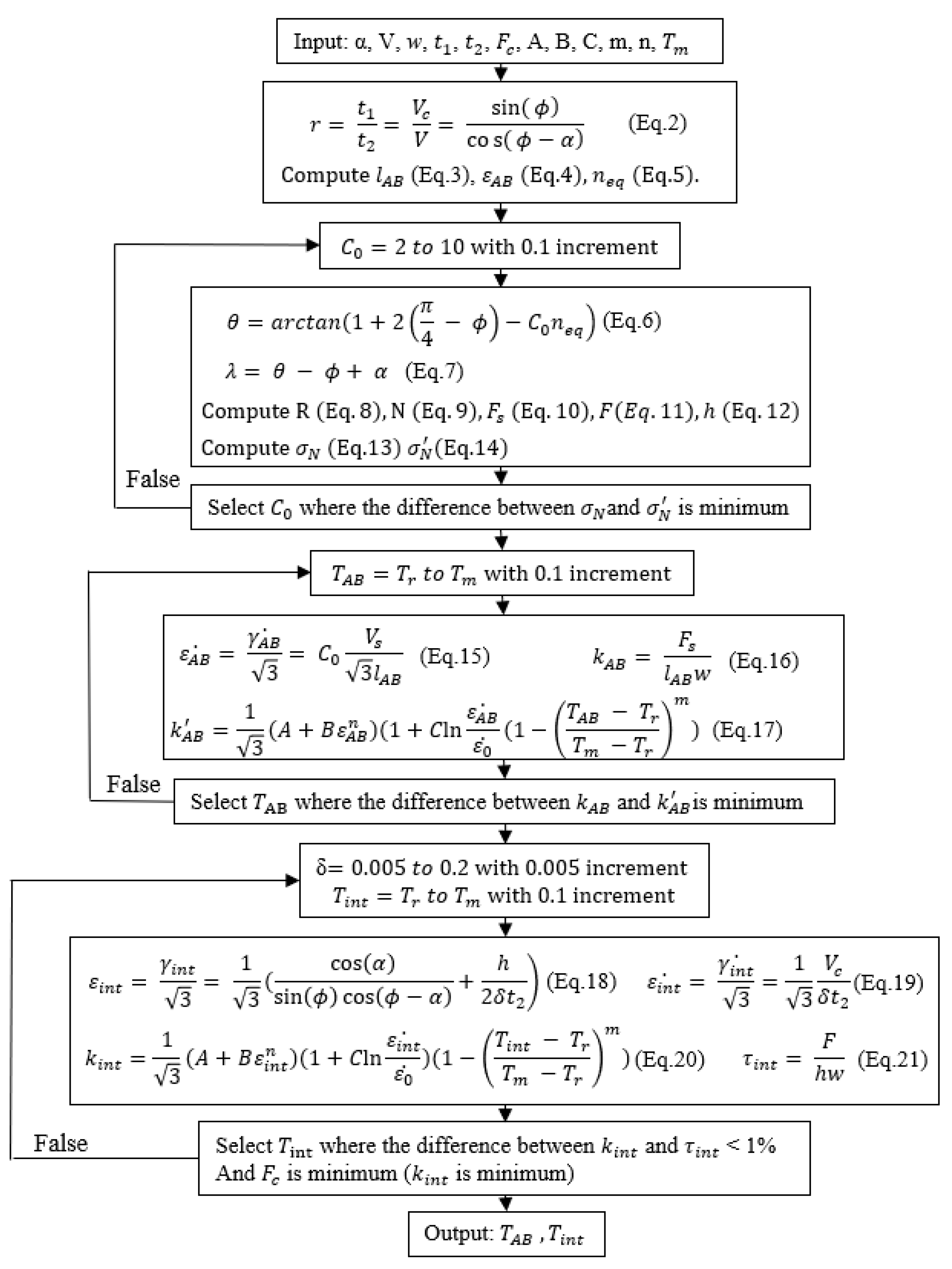
2. Methodology and Validation

The presented methodology predicted the average temperature at the PSZ, and the average temperature at the SSZ using experimental cutting forces, and experimental chip thicknesses. The PSZ and the SSZ are the two major heat sources in orthogonal cutting, and the average temperatures at these locations are needed to further predict machining forces and tool wear. Cutting conditions, including cutting velocity, depth of cut, width of cut, rake angle, and J–C model constants, were also used as inputs. This methodology was developed based on the J–C model and the chip formation model. The temperatures were determined when the difference between the predicted shear stress using the J–C model and that using the chip formation model reached an acceptably low value, as shown in Figure 5. The temperature at the PSZ and the temperature at the SSZ were determined with calculations of primary shear stress and of secondary shear stress, respectively.

The chip compression ratio was expressed as the equations below, with an assumption of constant material flow rate. The shear angle ($\varphi$) was then calculated as

$$r= \frac{t_1}{t_2}= \frac{V_c}{V}= \frac{\sin \left(\varphi \right)}{\cos \left(\varphi -\alpha \right)}.$$

(2)

The length of the shear zone ($l_{AB}$), and the strain (${\epsilon }_{AB}$) on the shear plane AB with the von Mises yield criterion were calculated as

$$l_{AB}=\frac{t_1}{\sin \varphi }.$$

(3)

$${\epsilon }_{AB}= \frac{{\gamma }_{AB}}{\sqrt{3}}= \frac{\cos \alpha }{2\sqrt{3}\sin \varphi \cos \left(\varphi -\alpha \right)}.$$

(4)

A strain hardening constant ($n_{eq}$) was expressed as

$$n_{eq}\approx \frac{nB{\epsilon }_{AB}^n}{\left(A+B{\epsilon }_{AB}^n\right)}.$$

(5)

The angles ($\theta \mathrm{and}\lambda$) in the chip formation model were expressed as

$$\theta =\arctan \left(1+2\left(\frac{\pi }{4} - \varphi \right)-C_0{n}_{eq}\right).$$

(6)

$$\lambda = \theta - \varphi + \alpha .$$

(7)

The resultant force (R), the normal force at the tool–chip interface (N), the shear force at the primary shear zone AB ($F_s$), and the frictional force at the tool–chip interface (F) were calculated as

$$R= \frac{F_c}{\cos \left(\lambda -\alpha \right)}.$$

(8)

$$N=R\cos \left(\lambda \right).$$

(9)

$$F_s=R\cos (\varphi +\lambda -\alpha ).$$

(10)

$$F=R\sin \left(\lambda \right).$$

(11)

The tool–chip contact length (h) at the tool–chip interface was expressed as

$$h=\frac{t_1\sin \theta }{\cos \mathsf{\lambda }\sin \varphi }\left(1+\frac{C_0{n}_{eq}}{3\left(1+2\left(\frac{\pi }{4}-\varphi \right)-C_0{n}_{eq}\right)}\right).$$

(12)

The normal stress (${\sigma }_N$) at the tool–chip interface was calculated as

$${\sigma }_N= \frac{N}{hw}.$$

(13)

The normal stress was found with the J–C model, with stress boundary conditions on the primary shear zone defined as

$${\sigma }_N^{\prime }= k_{AB}\left(1+\frac{\pi }{2} -2\alpha -2C_0{n}_{eq}\right).$$

(14)

The Oxley constant ($C_0$) was determined when the difference between the normal stress (${\sigma }_N$) and the normal stress $\left({\sigma }_N^{\prime }\right)$ was minimal. Then, the strain rate on the shear plane AB with the von Mises yield criterion was calculated as

$$\dot{{\epsilon }_{AB}}= \frac{\dot{{\gamma }_{AB}}}{\sqrt{3}}= C_0\frac{V_s}{\sqrt{3}{l}_{AB}}.$$

(15)

The shear flow stress ($k_{AB}$) was calculated based on the chip formation model as

$$k_{AB}= \frac{F_s}{l_{AB}w}.$$

(16)

The shear flow stress on the shear plane AB with the von Mises yield criterion was also calculated with the J–C model as

$$k_{AB}^{\prime }= \frac{{\sigma }_{AB}}{\sqrt{3}} =\frac{1}{\sqrt{3}}\left(A+B{\epsilon }_{AB}^n\right)\left(1+Cln\frac{\dot{{\epsilon }_{AB}}}{\dot{{\epsilon }_0}}\right)\left(1-{\left(\frac{T_{AB} - T_r}{T_m -T_r}\right)}^m\right).$$

(17)

The average temperature at the PSZ $\left(T_{AB}\right)$ was determined when the difference between the shear flow stress ($k_{AB}$) and the shear flow stress $(k_{AB}^{\prime }$) was minimal.

The strain and the strain rate at the tool–chip interface were expressed with the von Mises yield criterion as

$${\epsilon }_{int}= \frac{{\gamma }_{int}}{\sqrt{3}}= \frac{1}{\sqrt{3}}\left(\frac{\cos \left(\alpha \right)}{\sin \left(\varphi \right)\cos \left(\varphi -\alpha \right)}+\frac{h}{2\delta t_2}\right).$$

(18)

$$\dot{{\epsilon }_{int}}= \frac{\dot{{\gamma }_{int}}}{\sqrt{3}}=\frac{1}{\sqrt{3}}\frac{V_c}{\delta t_2}.$$

(19)

The flow stress at the SSZ was calculated with the J–C model as

$$k_{int}=\frac{1}{\sqrt{3}}\left(A+B{\epsilon }_{int}^n\right)\left(1+C\ln \frac{\dot{{\epsilon }_{int}}}{\dot{{\epsilon }_0}}\right)\left(1-{\left(\frac{T_{int} - T_r}{T_m -T_r}\right)}^m\right).$$

(20)

The shear stress at the SSZ was also calculated as

$${\tau }_{int}= \frac{F}{hw}.$$

(21)

The average temperature at the SSZ $\left(T_{int}\right)$ was determined when the difference between the shear flow stress (${\tau }_{int}$) and the shear flow stress ($k_{int}$) was minimal. The strain rate constant (δ) was determined by minimizing the cutting force ($F_c$), which was achieved by minimizing $k_{int}$ due to the positive correlation. $F_c$ was inversely calculated based on the equality between ${\tau }_{int}$ and $k_{int}$, and the chip formation model.

To test the proposed methodology, AISI 1045 steel and Al 6082-T6 aluminum were chosen for multiple tests for temperature predictions. The predicted temperatures were validated by comparing them to documented results found in the literature.

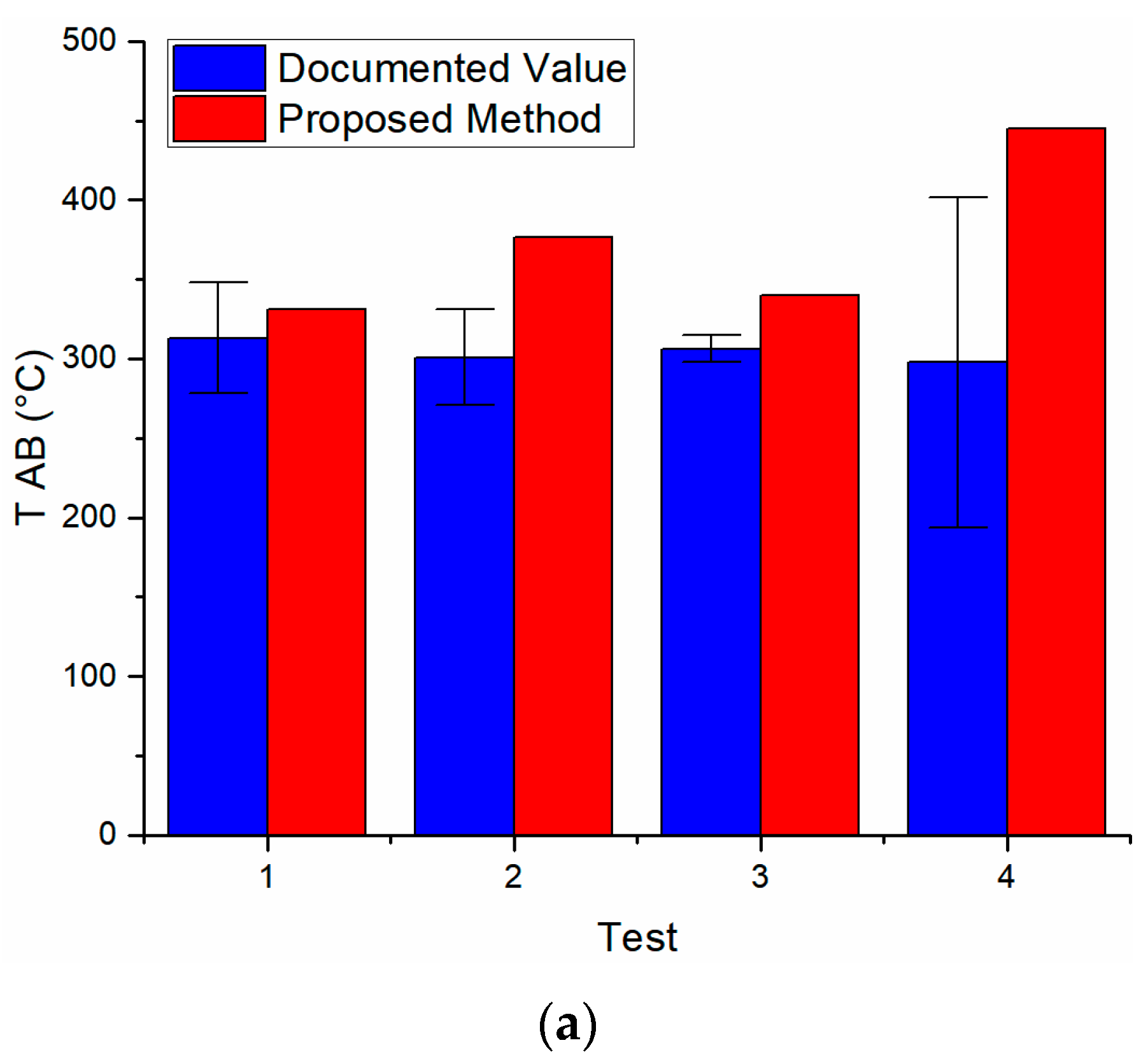
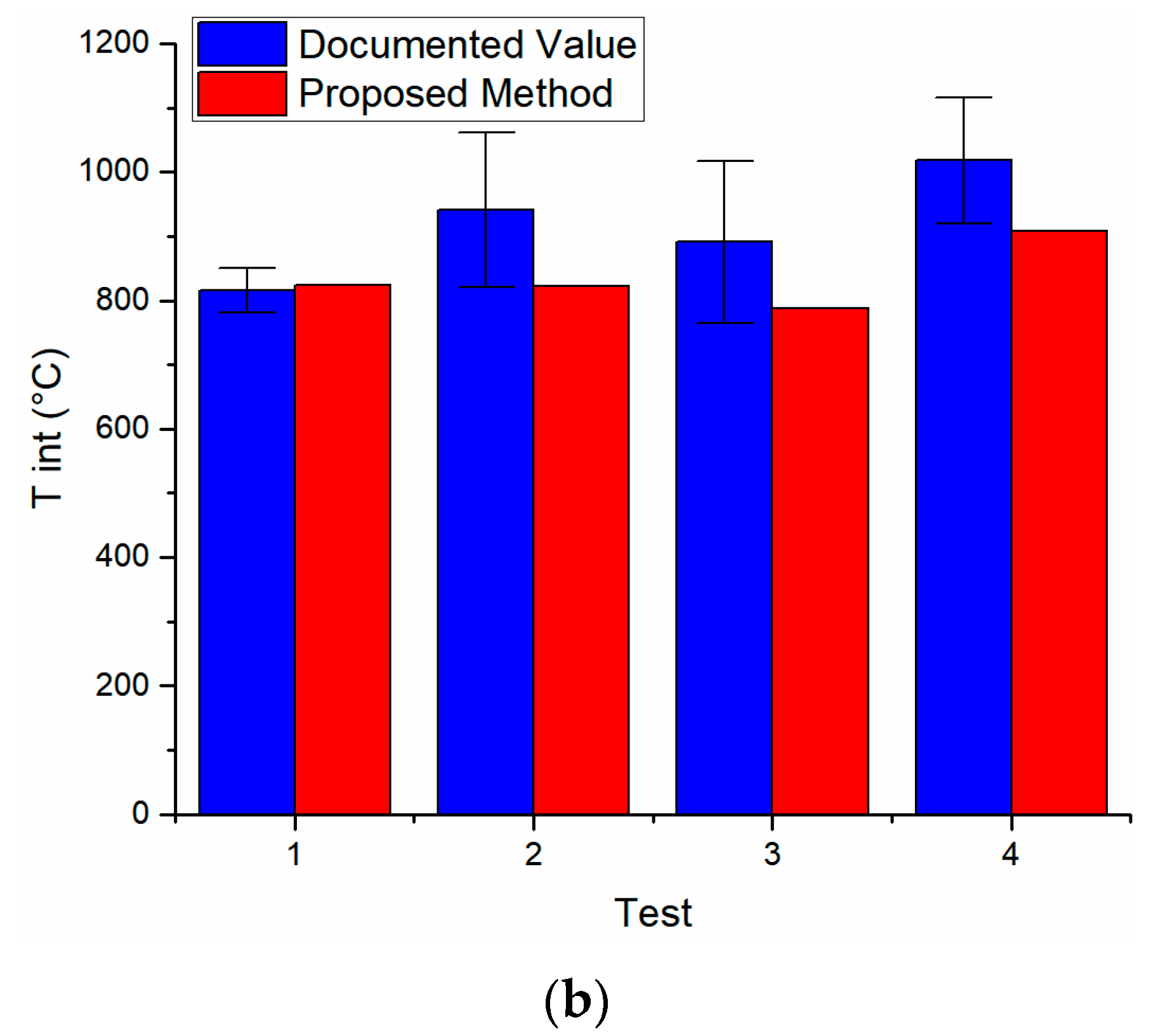
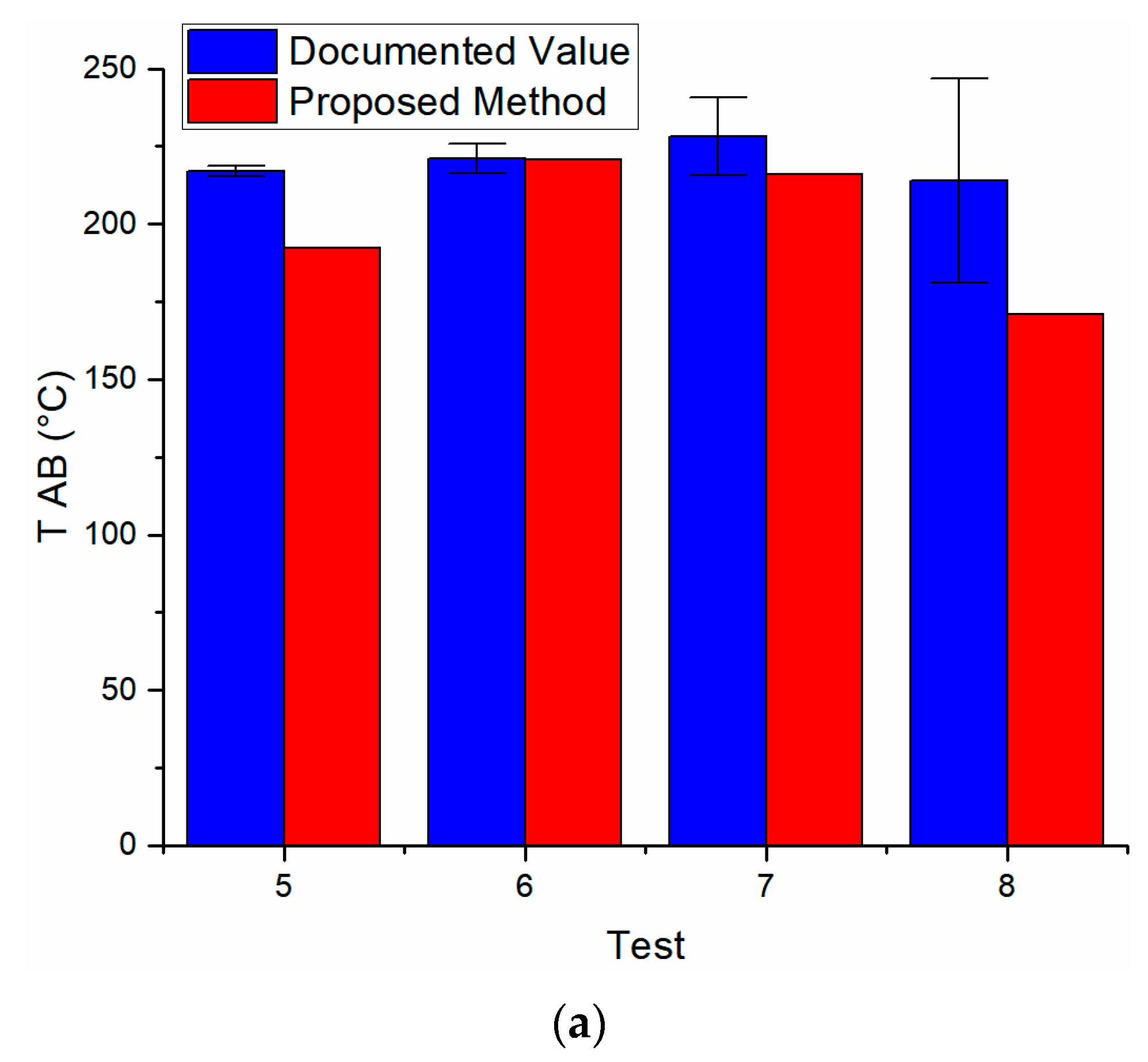
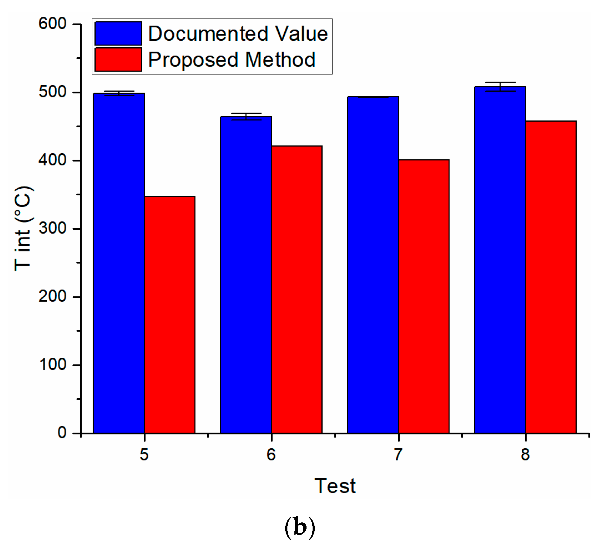
3. Results and Discussion

A computer program in MATLAB (2017) was developed to carry out the proposed methodology. The predictions of temperature distribution in machining AISI 1045 steel and Al 6082-T6 aluminum were made in multiple tests under various cutting conditions. As given in

Table 1. Johnson–Cook (J–C) model constants obtained from split Hopkinson pressure bar (SHPB) tests.

Materials	A (MPa)	B (MPa)	C	m	n	$\dot{{\mathit{\epsilon }}_0}$	${\mathit{T}}_{\mathit{m}}$ (°C)	${\mathit{T}}_{\mathit{r}}$ (°C)
ASIS 1045 Steel [40]	553.1	600.8	0.0134	1	0.234	1	1460	25
Al 6082-T6 Aluminum [37]	250	243.6	0.00747	1.31	0.17	1	582	25

, the J–C model constants of AISI 1045 steel and Al 6082-T6 aluminum were separately adopted from the literature, in which split Hopkinson pressure bar (SHPB) tests were conducted to determine the model constants [37,40]. The cutting conditions, including cutting velocity, depth of cut, width of cut, rake angle, and experimental measurements of force and chip thickness, are given in

Table 2. Cutting conditions and experimental measurements for machining AISI 1045 steel and Al 6082-T6 aluminum.

Material	Test	α (degs)	V (m/min)	w (mm)	${\mathit{t}}_1$ (mm)	${\mathit{t}}_2$ (mm)	Fc (N)	Ft (N)
AISI 1045 Steel	1	5	200	1.6	0.15	0.424	583	402
[36]	2	5	200	1.6	0.30	0.734	976	493
	3	5	300	1.6	0.15	0.389	539	326
	4	5	300	1.6	0.30	0.709	888	406
Al 6082-T6 Aluminum	5	8	120	3.0	0.20	0.52 *	552	384
[37]	6	8	240	3.0	0.40	0.76 *	795	300
	7	8	360	3.0	0.20	0.44 *	456	204
	8	8	360	3.0	0.40	0.64 *	768	276

Note: * represents values adopted from predictions in the literature [41].

[36,37]. The values of chip thickness in machining Al 6082-T6 aluminum were adopted from predictions in the literature due to the unavailability of experimental data, and were validated using machining force because the chip thickness was utilized as an intermediate variable in the force prediction in each test. The machining forces were validated by comparing them to experimental forces. Detailed information regarding the validation of documented values is given in Appendix A,

Table A1. Validation for the documented temperature using the force comparison [41,43].

AISI 1045 Steel	Fc_p (N)	Fc_e (N)	Error (%)	Al 6082-T6 Aluminum	Fc_p (N)	Fc_e (N)	Error (%)
1	464.69	583	20.29	5	550.00	552	0.36
2	816.02	976	16.39	6	767.00	795	3.52
3	431.67	539	19.91	7	443.00	456	2.85
4	766.03	888	13.74	8	719.00	768	6.38

.

The temperature distributions were predicted in four tests for each material. The predicted temperature at the PSZ ($T_{AB}$), the temperature at the SSZ ($T_{int}$), and other variables using the proposed method are listed in

Table 3. Predicted temperature distribution, and other process variables.

Test	${\mathit{T}}_{\mathit{A}\mathit{B}}$ (°C) R	${\mathit{T}}_{\mathit{A}\mathit{B}}$ (°C)	${\mathit{T}}_{\mathit{i}\mathit{n}\mathit{t}}$ (°C) R	${\mathit{T}}_{\mathit{i}\mathit{n}\mathit{t}}$ (°C)	ϕ (degs)	${\mathit{C}}_0$	δ
1	313.12	330.97	815.74	823.23	19.14	5.45	0.05
2	300.77	376.61	941.15	822.37	22.00	5.10	0.16
3	306.30	340.01	891.20	787.49	20.76	5.25	0.13
4	297.80	445.07	1018.00	908.47	22.78	5.00	0.10
5	217.00	192.40	498.00	346.80	20.76	7.58	0.14
6	221.00	220.64	464.00	421.35	20.02	6.33	0.17
7	228.00	216.01	493.00	400.90	24.39	6.90	0.06
8	198.00	171.00	508.00	457.72	31.67	5.72	0.08

Note: ^R denotes a reference value [41,42].

. To validate this methodology, the predicted values were individually compared to documented values. The documented temperatures were adopted from the literature [41,42], and validated by force comparisons because the chip thicknesses were intermediate variables in predicting machining forces. Good agreement was observed, as shown in Table A1. Force validation errors for AISI 1045 steel were found to be generally larger than those for Al 6082-T6 aluminum because of the differing prediction methods. The differing prediction methods are discussed further below. The error bars were added to the documented values due to the deviations of the inputs. The documented temperatures in the literature were determined using the predicted force, and the predicted chip thickness. The predictions using the proposed method utilized experimental force, and experimental chip thickness. Each error bar was calculated as the difference between the temperature using the adopted predicted values, and the temperature using the adopted experimental values in the proposed methodology. The comparisons of the temperatures in machining AISI 1045 steel and Al 6082-T6 aluminum are illustrated in Figure 6 and Figure 7, respectively. The deviations between the predicted temperatures and the documented values are discussed below, regarding the accuracy of the input force and the input chip thickness, and the methodology for calculating the documented values.

As shown in Figure 6, the predicted temperatures in the PSZ were larger than their corresponding documented values because the documented values were calculated using a heat partition equation ($T_{AB}=T_r+ \eta \mathsf{\Delta }{T}_{SZ}$), in which the heat partition ratio ($\eta$) was taken as 1, based on the best performance of the predictions [40]. This assumption gave acceptable prediction accuracy, as shown in Table A1, but it was not true in real cutting tests. On the other hand, the proposed method did not need this assumption for the temperature prediction. The other heat partition ratio ($\psi , T_{int}= T_r+ \mathsf{\Delta }{T}_{SZ}+ \psi \mathsf{\Delta }{T}_M$), used in calculating the temperature in the SSZ, was taken as 0.75, based on Xiong’s study [43]. This value was reported for their successful temperature prediction in the SSZ. The predicted temperatures in the SSZ were in good agreement with the documented values.

As shown in Figure 7, the documented temperatures were calculated using mean value calculations from a moving band heat source [41]. The predicted temperatures were in good agreement with the documented values; however, they were smaller than the documented values due to the assumption of a perfectly sharp cutting tool edge used in the proposed method. Smaller temperature and force predictions with an assumption of a perfectly sharp tool were also reported in previously published works [21,40,44].

The proposed method predicted temperatures using the J–C model and the chip formation model. The availability of J–C constants for metal materials commonly used in machining is increasing; however, it is still a major limitation. For materials such as AISI 316L steel and the Ti6Al4V titanium alloy, the J–C constants must be chosen from a large number of J–C constants available for the same material [45,46]. The error bars of documented temperatures in machining AISI 1045 steel were found to be generally larger than the error bars of documented temperatures in machining Al 6082-T6 aluminum because of the large input force errors in predicting temperatures for AISI 1045 steel. Therefore, the accurate measurements of cutting force and chip thickness were required for the temperature prediction.

4. Conclusions

In this work, an original methodology was presented for the prediction of temperature distribution in orthogonal cutting. Currently, the temperature distribution in machining is investigated with either arduous experiments using IR cameras, tool–chip interfaces, inserted thermocouples, etc., or inefficient numerical simulations, or complex analytical models, in which the determination of intermediate parameters remains difficult. This method was developed based on the J–C model and the chip formation model. The cutting conditions, the J–C model constants, the experimental cutting force, and the experimental chip thickness were used as inputs. The reliable and easily measurable cutting force and chip thickness were utilized in predicting the temperatures at the PSZ and at the SSZ. The temperatures were determined when the differences between the calculated shear stresses using the chip formation model and those using the J–C model reached acceptably low values. To validate the proposed methodology, machining data for AISI 1045 steel and Al 6082-T6 aluminum under various cutting conditions were adopted from the literature to predict the corresponding temperatures. The predicted temperatures were then compared to the documented results. Good agreement was observed for the tests with AISI 1045 steel and Al 6082-T6 aluminum. In light of the fact that cutting force and chip thickness are reliable and easily measurable, the calculations in the J–C model and the chip formation model were simple and easy to use. The proposed methodology has the advantages of less experimental complexity, less mathematical complexity, and high computational efficiency. In the future, this methodology can be employed in the analytical modeling of machining force and tool wear.

References

1. Stephenson, D.A.; Ali, A. Tool temperatures in interrupted metal cutting. J. Eng. Ind. 1992, 114, 127–136. [Google Scholar] [CrossRef]
2. Lezanski, P.; Shaw, M.C. Tool face temperatures in high speed milling. J. Eng. Ind. 1990, 112, 132–135. [Google Scholar] [CrossRef]
3. Yashiro, T.; Ogawa, T.; Sasahara, H. Temperature measurement of cutting tool and machined surface layer in milling of CFRP. Int. J. Mach. Tools Manuf. 2013, 70, 63–69. [Google Scholar] [CrossRef]
4. Kitagawa, T.; Kubo, A.; Maekawa, K. Temperature and wear of cutting tools in high-speed machining of Inconel 718 and Ti6Al6V2Sn. Wear 1997, 202, 142–148. [Google Scholar] [CrossRef]
5. Chen, W.C.; Tsao, C.C.; Liang, P.W. Determination of temperature distributions on the rake face of cutting tools using a remote method. Int. Commun. Heat Mass Transf. 1997, 24, 161–170. [Google Scholar] [CrossRef]
6. O’sullivan, D.; Cotterell, M. Temperature measurement in single point turning. J. Mater. Process. Technol. 2001, 118, 301–318. [Google Scholar] [CrossRef]
7. Jaspers, S.P.; Dautzenberg, J.H. Material behaviour in metal cutting: Strains, strain rates and temperatures in chip formation. J. Mater. Process. Technol. 2002, 121, 123–135. [Google Scholar] [CrossRef]
8. Lin, J.; Lee, S.L.; Weng, C.I. Estimation of cutting temperature in high speed machining. J. Mater. Process. Technol. 1992, 114, 289–296. [Google Scholar] [CrossRef]
9. Sutter, G.; Faure, L.; Molinari, A.; Ranc, N.; Pina, V. An experimental technique for the measurement of temperature fields for the orthogonal cutting in high speed machining. Int. J. Mach. Tools Manuf. 2003, 43, 671–678. [Google Scholar] [CrossRef] [Green Version]
10. Wright, P.K. Correlation of tempering effects with temperature distribution in steel cutting tools. J. Eng. Ind. 1978, 100, 131–136. [Google Scholar] [CrossRef]
11. Kato, S.; Yamaguchi, K.; Watanabe, Y.; Hiraiwa, Y. Measurement of temperature distribution within tool using powders of constant melting point. J. Eng. Ind. 1976, 98, 607–613. [Google Scholar] [CrossRef]
12. Dawson, P.R.; Malkin, S. Inclined moving heat source model for calculating metal cutting temperatures. J. Eng. Ind. 1984, 106, 179–186. [Google Scholar] [CrossRef]
13. Kim, K.W.; Sins, H.C. Development of a thermo-viscoplastic cutting model using finite element method. Int. J. Mach. Tools Manuf. 1996, 36, 379–397. [Google Scholar] [CrossRef]
14. Moriwaki, T.; Sugimura, N.; Luan, S. Combined stress, material flow and heat analysis of orthogonal micromachining of copper. CIRP Ann. Manuf. Technol. 1993, 42, 75–78. [Google Scholar] [CrossRef]
15. Lei, S.; Shin, Y.C.; Incropera, F.P. Thermo-mechanical modeling of orthogonal machining process by finite element analysis. Int. J. Mach. Tools Manuf. 1999, 39, 731–750. [Google Scholar] [CrossRef]
16. Levy, E.K.; Tsai, C.L.; Groover, M.P. Analytical investigation of the effect of tool wear on the temperature variations in a metal cutting tool. J. Eng. Ind. 1976, 98, 251–257. [Google Scholar] [CrossRef]
17. Chan, C.L.; Chandra, A. A boundary element method analysis of the thermal aspects of metal cutting processes. J. Eng. Ind. 1991, 113, 311–319. [Google Scholar] [CrossRef]
18. Umbrello, D.; Filice, L.; Rizzuti, S.; Micari, F.; Settineri, L. On the effectiveness of finite element simulation of orthogonal cutting with particular reference to temperature prediction. J. Mater. Process. Technol. 2007, 189, 284–291. [Google Scholar] [CrossRef]
19. Kim, D.H.; Lee, C.M. A study of cutting force and preheating-temperature prediction for laser-assisted milling of Inconel 718 and AISI 1045 steel. Int. J. Heat Mass Transf. 2014, 71, 264–274. [Google Scholar] [CrossRef]
20. Yang, J.; Sun, S.; Brandt, M.; Yan, W. Experimental investigation and 3D finite element prediction of the heat affected zone during laser assisted machining of Ti6Al4V alloy. J. Mater. Process. Technol. 2010, 210, 2215–2222. [Google Scholar] [CrossRef]
21. Özel, T.; Zeren, E. Finite element modeling the influence of edge roundness on the stress and temperature fields induced by high-speed machining. Int. J. Adv. Manuf. Technol. 2007, 35, 255–267. [Google Scholar] [CrossRef]
22. Attia, M.H.; Kops, L. A new approach to cutting temperature prediction considering the thermal constriction phenomenon in multi-layer coated tools. CIRP Ann. Manuf. Technol. 2004, 53, 47–52. [Google Scholar] [CrossRef]
23. Wiener, J.H. Shear-plane temperature distribution in orthogonal cutting. Trans. ASME 1955, 77, 1331–1341. [Google Scholar]
24. Boothroyd, G. Fundamentals of Metal Machining and Machine Tools; Scripta Book Company: Washington, DC, USA, 1975; ISBN 9780070064980. [Google Scholar]
25. Radulescu, R.; Kapoor, S.G. An analytical model for prediction of tool temperature fields during continuous and interrupted cutting. J. Eng. Ind. 1994, 116, 135–143. [Google Scholar] [CrossRef]
26. Stephenson, D.A.; Jen, T.C.; Lavine, A.S. Cutting tool temperatures in contour turning: Transient analysis and experimental verification. J. Manuf. Sci. Eng. 1997, 119, 494–501. [Google Scholar] [CrossRef]
27. Komanduri, R.; Hou, Z.B. Thermal modeling of the metal cutting process—Part III: Temperature rise distribution due to the combined effects of shear plane heat source and the tool–chip interface frictional heat source. Int. J. Mech. Sci. 2001, 43, 89–107. [Google Scholar] [CrossRef]
28. Hahn, R.S. On the temperature developed at the shear plane in the metal cutting process. J. Appl. Mech. Trans. ASME 1951, 18, 661–666. [Google Scholar]
29. Jaeger, C. Conduction of Heat in Solids; Oxford University Press: Oxford, UK, 1959; ISBN 9780198533689. [Google Scholar]
30. Huang, Y.; Liang, S.Y. Cutting forces modeling considering the effect of tool thermal property—Application to CBN hard turning. Int. J. Mach. Tools Manuf. 2003, 43, 307–315. [Google Scholar] [CrossRef]
31. Li, K.M.; Liang, S.Y. Modeling of cutting forces in near dry machining under tool wear effect. Int. J. Mach. Tools Manuf. 2007, 47, 1292–1301. [Google Scholar] [CrossRef]
32. Huang, Y.; Liang, S.Y. Cutting temperature modeling based on non-uniform heat intensity and partition ratio. Mach. Sci. Technol. 2005, 9, 301–323. [Google Scholar] [CrossRef]
33. Korkut, I.; Acır, A.; Boy, M. Application of regression and artificial neural network analysis in modelling of tool–chip interface temperature in machining. Exp. Syst. Appl. 2011, 38, 11651–11656. [Google Scholar] [CrossRef]
34. Oxley, P.L.B. The Mechanics of Machining: An Analytical Approach to Assessing Machinability; Ellis Horwood Ltd.: Chichester, UK, 1989; ISBN 0745800076. [Google Scholar]
35. Calculating the shear angle in orthogonal metal cutting from fundamental stress-strain-strain rate properties of the work material. Available online: https://dspace.lib.cranfield.ac.uk/handle/1826/12577 (accessed on 23 April 2018).
36. Ivester, R.W.; Kennedy, M.; Davies, M.; Stevenson, R.; Thiele, J.; Furness, R.; Athavale, S. Assessment of machining models: Progress report. Mach. Sci. Technol. 2000, 4, 511–538. [Google Scholar] [CrossRef]
37. Adibi-Sedeh, A.H.; Madhavan, V.; Bahr, B. Extension of Oxley’s analysis of machining to use different material models. J. Manuf. Sci. Eng. 2003, 125, 656–666. [Google Scholar] [CrossRef]
38. Mia, M.; Dhar, N.R. Response surface and neural network based predictive models of cutting temperature in hard turning. J. Adv. Res. 2016, 7, 1035–1044. [Google Scholar] [CrossRef] [PubMed] [Green Version]
39. M’saoubi, R.; Chandrasekaran, H. Investigation of the effects of tool micro-geometry and coating on tool temperature during orthogonal turning of quenched and tempered steel. Int. J. Mach. Tools Manuf. 2004, 44, 213–224. [Google Scholar] [CrossRef]
40. Jaspers, S.P.; Dautzenberg, J.H. Material behaviour in conditions similar to metal cutting: Flow stress in the primary shear zone. J. Mater. Process. Technol. 2002, 122, 322–330. [Google Scholar] [CrossRef]
41. Karpat, Y.; Özel, T. Predictive analytical and thermal modeling of orthogonal cutting process—Part I: Predictions of tool forces, stresses, and temperature distributions. J. Manuf. Sci. Eng. 2006, 128, 435–444. [Google Scholar] [CrossRef]
42. Aydın, M. Cutting temperature analysis considering the improved Oxley’s predictive machining theory. J. Braz. Soc. Mech. Sci. Eng. 2016, 38, 2435–2448. [Google Scholar] [CrossRef]
43. Xiong, L.; Wang, J.; Gan, Y.; Li, B.; Fang, N. Improvement of algorithm and prediction precision of an extended Oxley’s theoretical model. Int. J. Adv. Manuf. Technol. 2015, 77, 1–3. [Google Scholar] [CrossRef]
44. Ning, J.; Liang, S.Y. Model-driven determination of Johnson-Cook material constants using temperature and force measurements. Int. J. Adv. Manuf. Technol. 2018, 1–8. [Google Scholar] [CrossRef]
45. Umbrello, D.; M’saoubi, R.; Outeiro, J.C. The influence of Johnson–Cook material constants on finite element simulation of machining of AISI 316L steel. Int. J. Mach. Tools Manuf. 2007, 47, 462–570. [Google Scholar] [CrossRef]
46. Ducobu, F.; Rivière-Lorphèvre, E.; Filippi, E. On the importance of the choice of the parameters of the Johnson-Cook constitutive model and their influence on the results of a Ti6Al4V orthogonal cutting model. Int. J. Mech. Sci. 2017, 122, 143–155. [Google Scholar] [CrossRef]
Figure 1. The chip formation model for orthogonal cutting [34].
Jmmp 02 00037 g001
Figure 2. The parallel-sided shear zone model [35].
Jmmp 02 00037 g002
Figure 3. Schematic drawing of the temperature measurement with an infrared camera on the chip’s free side in orthogonal cutting [7].
Jmmp 02 00037 g003
Figure 4. Schematic drawing of the temperature measurement using a tool–work thermocouple technique [38]. To enforce orthogonal cutting, a tubular workpiece with uniform wall thickness was used [39]. The cutting force was in the tangential direction of the tubular workpiece, and perpendicular to the tool’s cutting edge, as shown in the side-view drawing (blue box).
Jmmp 02 00037 g004
Figure 5. Flowchart for the algorithm of temperature prediction based on the Johnson–Cook (J–C) model and the chip formation model.
Jmmp 02 00037 g005
Figure 6. Temperature predictions for machining AISI 1045 steel. The average temperatures in the primary shear zone are shown in (a); The average temperatures in the secondary shear zone are shown in (b). The documented values are predicted values adopted from the literature [42].
Jmmp 02 00037 g006aJmmp 02 00037 g006b
Figure 7. Temperature predictions for machining Al 6082-T6 aluminum. The average temperatures in the primary shear zone are shown in (a); The average temperatures in the secondary shear zone are shown in (b). The documented values are predicted values adopted from the literature [41].
Jmmp 02 00037 g007aJmmp 02 00037 g007b