Modelling Machine Tools using Structure Integrated Sensors for Fast Calibration

Abstract

Monitoring of the relative deviation between commanded and actual tool tip position, which limits the volumetric performance of the machine tool, enables the use of contemporary methods of compensation to reduce tolerance mismatch and the uncertainties of on-machine measurements. The development of a primarily optical sensor setup capable of being integrated into the machine structure without limiting its operating range is presented. The use of a frequency-modulating interferometer and photosensitive arrays in combination with a Gaussian laser beam allows for fast and automated online measurements of the axes’ motion errors and thermal conditions with comparable accuracy, lower cost, and smaller dimensions as compared to state-of-the-art optical measuring instruments for offline machine tool calibration. The development is tested through simulation of the sensor setup based on raytracing and Monte-Carlo techniques.

1. Introduction

At any given functional point within the working space of a machine tool, a relative deviation between the desired and actual tool tip position is expected. This is due to various error sources, such as for instance dynamic forces, thermo-mechanical deformations, unconsidered loads, the shortcomings of motion control, and inherent kinematic errors [1]. The upper limit of the resulting deviation per axis is defined as volumetric accuracy, and determines the volumetric performance [2]. Insufficient volumetric performance can be a cause of tolerance mismatch and should hence be avoided. This can be achieved for non-dynamic and repeatable influences by calibrating the machine tool and then compensating the known error motions via the motion control system. As previously mentioned, error sources are likely to vary over time and the calibration should be repeated regularly. Different techniques currently exist, and can be subdivided in methods using calibrated artifacts, e.g., ball-plates, and optical methods, e.g., interferometric multilateration [1,3].

All methods have two major drawbacks in common. Firstly, the production process has to be interrupted and the setup prepared for calibration, which means an unfavourable expenditure of time. Moreover, as defined in ISO 230-1:2012(en), the machine is calibrated under a »no-load or quasi-static condition« and may show significantly different behaviour compared to normal use during manufacturing [2]. The authors’ concept is to (permanently) integrate optical sensors into the machine tool’s axes, which in contrast to traditional scales are also capable of measuring transversal and angular movements of the axes’ slides. This concept addresses the described drawbacks and will be presented in this paper. The complete idea is described for three-axis Cartesian machine tools and reduced to the measurement of error motions for a single axis. Thereafter, a specific hardware layout for integration is described. In Section 4, the use of industrial cameras instead of quadrant detectors for the measurement of lateral laser beam displacement is suggested. This concept is implemented in a prototype, which is used for competitive measurements in Section 6.

2. The Concept of Integrated Optical Sensors for Three-Axis Machine Tool Calibration

The first underlying assumption of the elaborated concept is that all components of a three-axis Cartesian machine tool can be modelled as rigid bodies. Thus, the resulting deviation at the functional point can be stated as a superposition of contributions from the linear axes’ individual error motions and squareness relations [4]. As a rigid body, every axis slide has six degrees of freedom for error motions: one linear positioning error motion parallel to the direction of motion, two perpendicular straightness error motions, and three angular error motions denominated yaw, pitch, and roll [2].

Hence, the calibration of the machine tool is reduced to the calibration of its linear axes and the application of a mathematical model according to the structural loop. This leads to the second fundament of the concept: If a sufficiently compact setup capable of measuring all error motions is integrated into the axes, the calibration setup can be made permanent without obstructing the working volume. There is no need to change the tool for an optical component, e.g. a reflector, and the measurement may be performed in a short time while the machine tool is not being used or even during operation. Using environmental compensation for optical measurements, the thermal behaviour of the axes can also be monitored by repeating the measurement sequence if the environmental conditions are expected to vary [5]. In the current state of the project, squareness errors between axes are excluded, which are especially inappropriate for large machine tools. In the future, the authors aim to slightly modify the individual base and head units using mirrors, pentaprisms, and beamsplitters, such that the visible laser propagates from a single source along the kinematic chain of the machine tool, serving as optical reference frame.

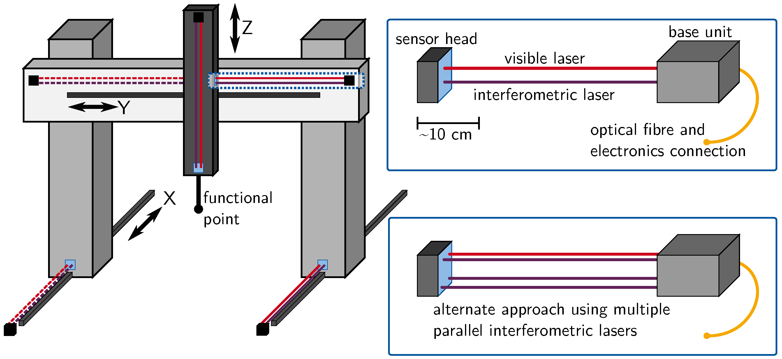
Figure 1 shows a sketch of the concept for a three-axis Cartesian machine of a gantry type. This machine type was chosen as a test carrier for a first implementation, but the application of the concept to any configuration of accessible linear axes is possible. At least one measurement line per direction of movement must be installed if the sensor setup is capable of measuring all error motions simultaneously. For this purpose, the layouts discussed in Section 3 are suitable. Their complexity can be reduced if multiple measurement lines (sketched in Figure 1 as dashed lines) are used, as angular movements can be calculated from the difference in linear movements. It is assumed that angular motions are of a small absolute value so that trigonometric functions can be approximated to the linear order of their Taylor series expansions. The calculation of the total deviation based on the axes’ individual contributions is state-of-the-art and not further discussed here, and nor is the data processing in the motion control unit [6].

3. Approach for a Single-Axis Sensor Setup

In nearly all modern machine tool calibration devices, optical techniques prevail [7,8]. The elaborated concept also primarily uses optical components for the following reasons:

• Optical sensors are able to provide a high resolution even for measurements concerning the largest existing machine tools.
• In contrast to setups with rigid components, e.g. glass scales, they are more adaptable to different machine tools and are reconfigurable.
• The decreasing size of active components, particularly emerging fibre-based interferometers, enables the complete setup to be sufficiently small for temporary or even permanent integration.

Both Renishaw with its XM-60 system [9] and Automated Preicision (API) with the XD-Laser [10] offer commercial devices using optical principles for simultaneous calibration of linear axes in six degrees of freedom (6-DOF). While their measurement uncertainty is low enough for the implementation of the concept suggested in Figure 1, the cost of three systems is not viable. Moreover, these devices are designed for offline maintenenance use and provide very little flexibilty to adapt the measurement setup to the structure of the machine tool.

Chen et al. present a 6-DOF measurement setup using a single laser source, three fixed position sensing devices, two fixed beamsplitters, and one fixed mirror in combination with one additional mirror attached to the moving stage [11]. Li et al. show a 6-DOF surface encoder using a fixed sensor consisting of multiple optical components and a scale grating attached to the moving element [12]. Gao et al. designed a 6-DOF measurement method for X-Y stages using nine interferometers [13]. All three sensor assemblies can only partially be used for the discussed integration purposes, as their limited measurement range would reduce the applicability to small machine tools. For linear axes with larger travel ranges, Kuang et al. developed a 4-DOF system measuring straightness, yaw, and pitch error motions [14]. The combination of a semi-translucent mirror, beamsplitter, and position sensing devices for capturing angular error motions is very similar to the setup presented throughout this paper, but the measurement of straightness error motions follows an indirect principle using a corner cube retroreflector. The following approaches are regarded as appropriate for practical tests of the concept:

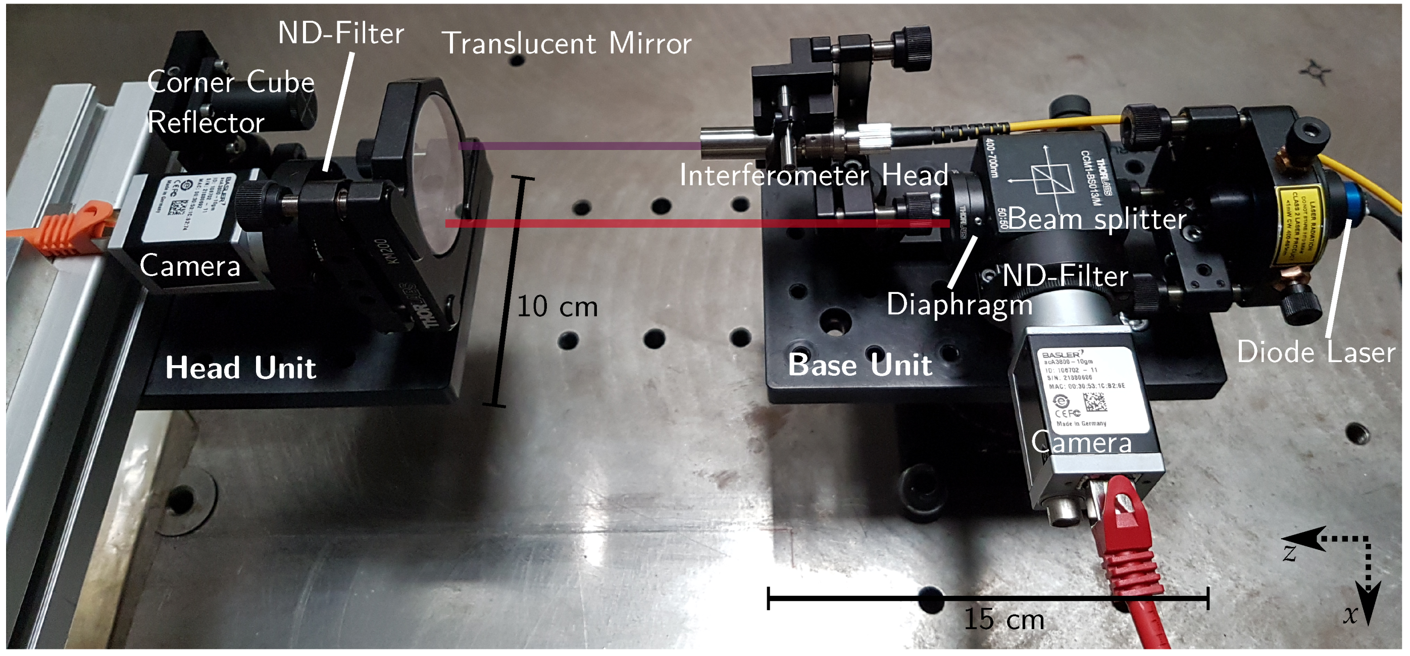
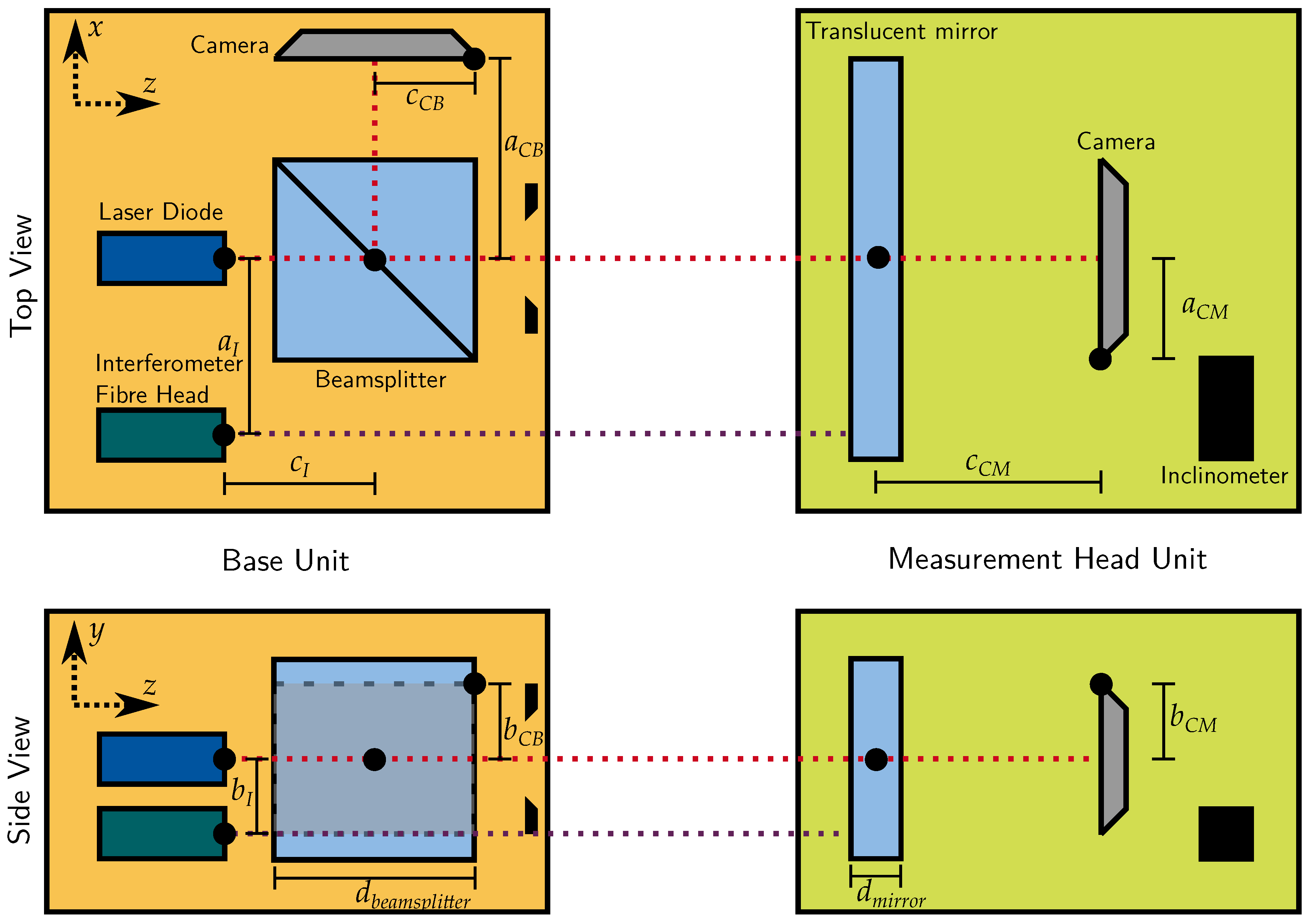
• Figure 4 shows the prototype implementation of a combination of a visible laser with two position sensing devices, placed in either the fixed base unit or the mobile sensor head. The linear positioning error motion is measured with the interferometer, while the camera in the sensor head can be used to measure the straightness error motions. Yaw and pitch are obtained by evaluating the displacement of the reflected beam on the camera in the base unit against the distance between both units. The inclinometer measures the roll error motion for non-vertical axes and can be of an arbitrary form, e.g. based on gravitational gauges. For vertical axes showing a significant roll error motion, the use of an optical principle is a possible alternative.
• The first approach can be modified to use only one position sensing device and three parallel laser beams used for interferometry to measure two angular error motions (pitch and yaw). Depending on the devices used, this variant may offer lower measurement uncertainties.
• The sensor setup proposed by Kuang et al. can be combined with an interferometer and a techique to measure roll error motions [14].
• Using multiple distributed sensor setups per direction of motion, the needed components change, e.g. the pitch of the gantry can be evaluated by measuring the travelled distance on both sides (see Figure 1).
• If one or more axes of the machine tool possess a built-in linear encoder capable of capturing positioning error motions, depending on the concept, the use of interferometry can be reduced or completely omitted and replaced by the encoder’s information.

In all cases, the magnitude of the error motions can be determined from the sensor readings by applying the laws of reflection and refraction. Pitch and yaw error motions of the sensor head in the first approach (Figure 4) are evaluated through:

$$\begin{array}{cc}\hfill {\phi }_{pitch}& =\frac{1}{2}\frac{-u_{base}+c_{CB}}{l+c_I+a_{CB}-\left(1-\frac{n_{ambient}}{n_{beamsplitter}}\right)·d_{beamsplitter}}\hfill \end{array}$$

(1)

$$\begin{array}{cc}\hfill {\phi }_{yaw}& =\frac{1}{2}\frac{-v_{base}+b_{CB}}{l+c_I+a_{CB}-\left(1-\frac{n_{ambient}}{n_{beamsplitter}}\right)·d_{beamsplitter}}\hfill \end{array}$$

(2)

Here, $u_{base}$ and $v_{base}$ denote the displacement of the laser spot on the position sensing device in the base unit. The distance measured by the interferometer is referenced as l and $d_{beamsplitter}$ denotes the length of the beam splitter cube. The corresponding refractive indices are stated as $n_{ambient}$ and $n_{beamsplitter}$, whereas $a_{CB},b_{CB},c_{CB},a_{CM},b_{CM}$, and $c_{CM}$ are calibration constants of the setup (see Figure 2). The yaw movement is obtained in the same way using the vertical beam displacement. Maintaining the naming convention and denoting the laser displacement on the position sensing device in the head unit by $u_{head}$ and $v_{head}$, the horizontal (x) and vertical (y) straightness are calculated as:

$$\begin{array}{cc}\hfill x_{straightness}& =u_{head}+a_{CM}+{\phi }_{pitch}·\left(c_{CM}-\left(1-\frac{n_{ambient}}{n_{mirror}}\right)·d_{mirror}\right)\hfill \end{array}$$

(3)

$$\begin{array}{cc}\hfill y_{straightness}& =v_{head}-b_{CM}+{\phi }_{yaw}·\left(c_{CM}-\left(1-\frac{n_{ambient}}{n_{mirror}}\right)·d_{mirror}\right)\hfill \end{array}$$

(4)

Linear positioning and roll error motions are trivially obtained from the interferometer and inclinometer readings. A virtual implementation of the sensor setup discussed in Section 5 is used to validate the mathematical formulation and propagation of uncertainties for different layouts.

For a compact base unit, the use of a fibre-based interferometer is advantageous. By only including the collimating fibre-head in the axis-integrated setup, the laser source and evaluation unit are placed outside the machine. One source can be used for multiple measurement lines and help reduce costs. Moreover, frequency modulating devices provide the possibility of absolute distance measurements, omitting the need for initial referencing of the setup [7].

4. Position Sensing Devices: Quadrant Detector vs. Industrial Cameras

The sensor setup presented in Section 3 as well as a wide range of metrological devices in general use position sensing devices to determine the lateral displacement between a laser beam and its target. During the first experiments, a Thorlabs PDQ30C [15] quadrant detector in combination with an infrared laser (1530 nm wavelength) beam was characterized and significant non-linear behaviour observed, leading to systematic measurement errors of several tens of micrometers.

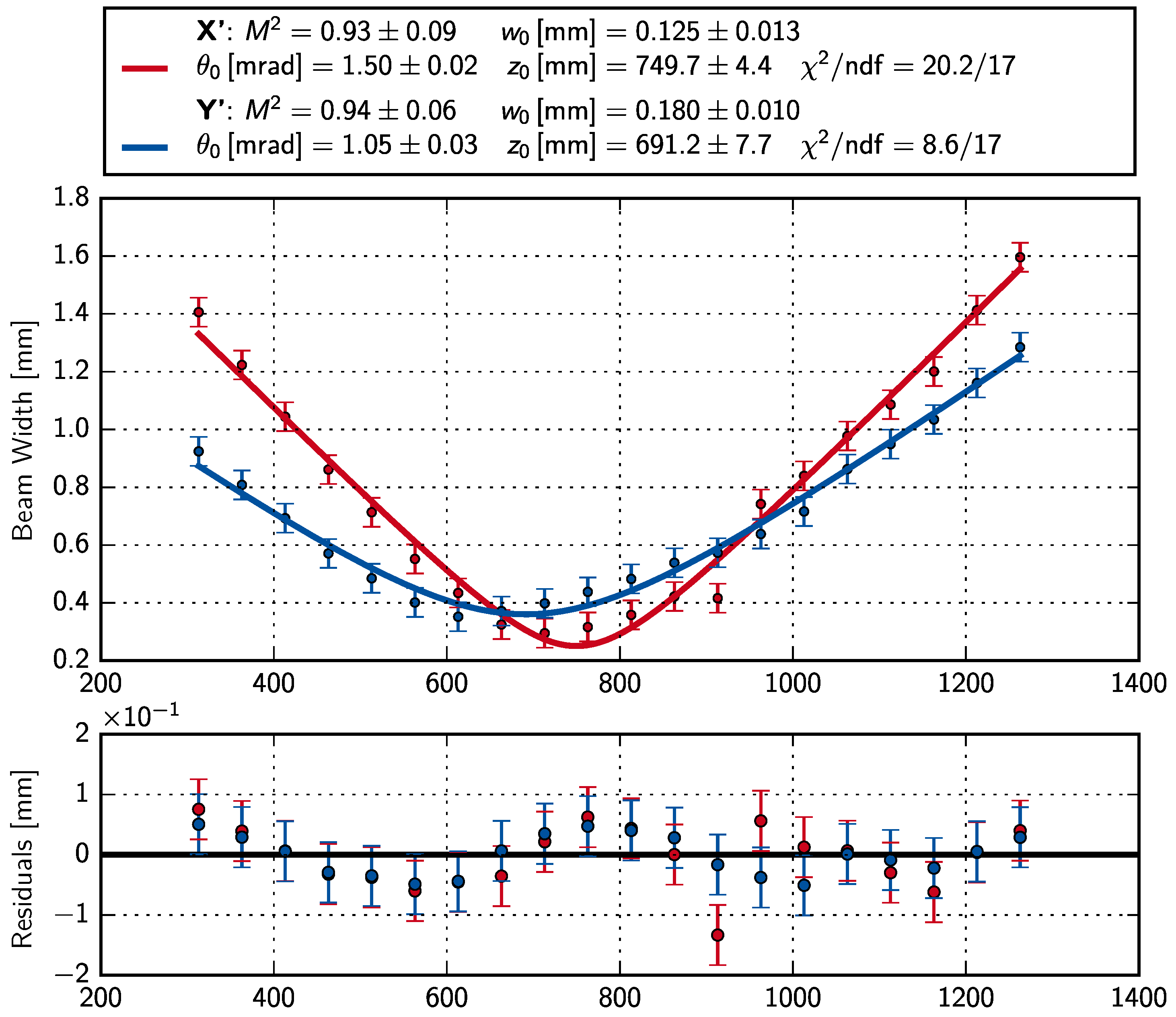
This effect can be attributed to the principle of a quadrant detector assuming that the intensity is distributed uniformly across the profile of the incident beam. However, for most lasers the model of a Gaussian beam is more appropriate (Figure 3) [16]. The beam’s respective spot size along the axis of propagation z is expressed as beam radius $w\left(z\right)$ following a hyperbolic relation:

$$\begin{array}{cc}\hfill w^2\left(z\right):& =w_0^2\left(1+{\left(\frac{z-z_0}{z_R}\right)}^2\right)=w_0^2+{\theta }_0^2{z}^2\hfill \end{array}$$

(5)

$$\begin{array}{cc}\hfill w_0^2:& =\frac{2z_R}{k},k=\frac{2\pi }{\lambda },{\theta }_0=arctan\left(\frac{w_0}{z_R}\right)\hfill \end{array}$$

(6)

In the above equations, $\lambda$ denotes the wavelength. The beam waist $w_0$ is defined as the beam radius at the focal point $z=z_0$, and hence at its smallest extension. The divergence of the beam is characterized by the Rayleigh length $z_R$, which is the distance from the focal point at which the spot area has doubled and together with $z_R$ defines the angle of divergence ${\theta }_0$. With these parameters, the distribution of intensity across the beam profile can be expressed with a structure similar to a Gaussian probability distribution:

$$\begin{array}{cc}\hfill I\left(r,z\right)& =I_0\frac{w_0^2}{w^2\left(z\right)}exp\left(-\frac{2r^2}{w^2\left(z\right)}\right)\hfill \end{array}$$

(7)

The problem arising using quadrant detectors can be exemplified mathematically along one axis, assuming that the detector consists of two photosensitive halves with signals $I_{+}$ and $I_{-}$, and has a range of $\pm R$ around zero. Interpreting w as an effective beam radius along the detector axis, the signal S is proportional to the displacement of the beam’s centre and can be computed from the difference of intensities distributed according to Equation (7):

$$\begin{array}{cc}\hfill S\left(x,w\right)\propto I_{+}-I_{-}\propto & \frac{1}{w^2}\underset{0}{\overset{R}{\int }}exp\left(-\frac{2{\left(s-x\right)}^2}{w^2}\right)\mathrm{d}s-\frac{1}{w^2}\underset{-R}{\overset{0}{\int }}exp\left(-\frac{2{\left(s-x\right)}^2}{w^2}\right)\mathrm{d}s\hfill \end{array}$$

(8)

$$\begin{array}{cc}\hfill \stackrel{-R<x<R}{=}& \frac{1}{w^2}\underset{0}{\overset{2x}{\int }}exp\left(-\frac{2{\left(s-x\right)}^2}{w^2}\right)\mathrm{d}s\stackrel{\frac{x^2}{w^2}\ll 1}{\to }\frac{8x}{w^2}\stackrel{z\gg z_R}{\approx }\frac{8\pi }{z_R·\lambda }·\frac{x}{z^2}\hfill \end{array}$$

(9)

Equation (8) unveils a clear non-linear relation between the beam position and the sensor signal, which may only be approximated linearly if the displacement is much smaller than the beam radius and the latter is constant. For a typical laser, neither of these conditions hold, as the product of beam waist $w_0$ and angle of divergence $\theta$ is limited by the beam quality parameter $M^2$ [17]:

$$\begin{array}{c}\hfill M^2:=w_0·\theta ·\frac{\pi }{\lambda }\ge 1\end{array}$$

(10)

A measurement sequence to determine $M^2$ according to ISO 11146-1 was carried out for the Premier LC laser diode (635 nm wavelength) manufactured by Global Laser and used for the prototype setup in Section 6 (Appendix A) [18]. The results confirm the behaviour of a Gaussian laser beam with a quality parameter close to optimal ($M_{x^{\prime }}^2=0.93\pm 0.09$ and $M_{y^{\prime }}^2=0.94\pm 0.06$).

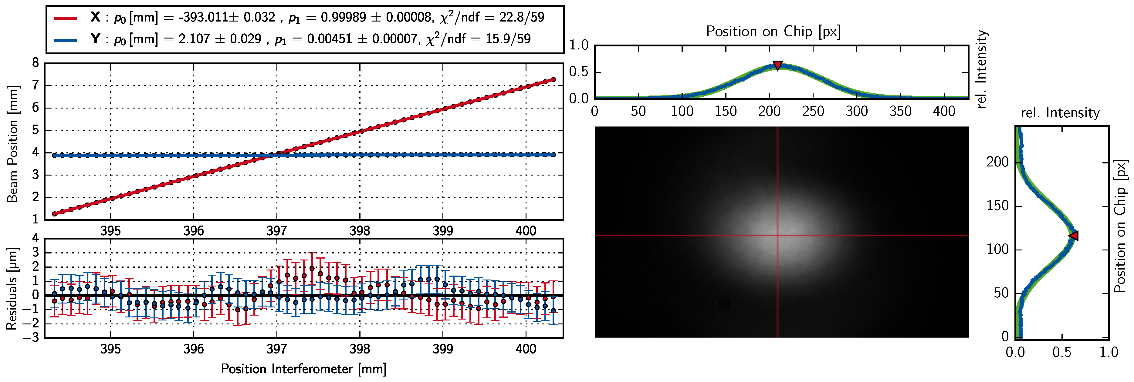
As an alternative, industrial charge-coupled-device (CCD) or complementary metal-oxide-semiconductor (CMOS) cameras in combination with neutral density filters capturing a digital image of the beam’s cross-section [19] are investigated. A sample is shown in Figure 3. The image is regarded as histogram of a quantity following a bivariate Gaussian distribution. After removing noise, e.g. ambient light, by applying a threshold, the location and hence movement of the beam centre can be obtained by calculating the first algebraic moments of the histogram and converted into dimensional coordinates by multiplying with the pixel pitch of the camera [20]. The divergent beam radius imposes no problem as long as at least $95\%$ of the beam cross-section is captured.

This idea was validated in an experimental setup using the aforementioned laser diode directed onto a Basler piA2400-12gm [21] camera with a pixel pitch of $3.45\mathsf{\mu }\mathrm{m}$. The camera was placed on a linear positioning stage orthogonally oriented to the beam direction, leading to a horizontal movement which was tracked using an Etalon Absolute Multiline interferometer [22]. Figure 4 shows the results of one run of the test series as a direct comparison of the displacement measured by both devices. An uncertainty ($k=1$) of $1\mathsf{\mu }\mathrm{m}$ is attributed to the interferometer and $1\mathsf{\mu }\mathrm{m}$ is estimated as uncertainty for camera data. The uncertainties of the positioning stage do not influence the measurements as directly comparing the readings of camera and interferometer omit the need of the positioning stage’s control data for evaluation.

The expected linear behaviour in horizontal and constant behaviour in vertical direction was confirmed by performing a chi-square minimization on the obtained data showing excellent agreement of assumed model and measured values (${\chi }^2/\mathrm{ndf}\approx 0.5$). Within a range of $7\mathrm{mm}$, the displacement of the beam centre can be measured with an uncertainty ($k=1$) of $1\mathsf{\mu }\mathrm{m}$ + $1\mathsf{\mu }\mathrm{m}/\mathrm{mm}$ of the displacement range.

Hence the combination of visible laser diode and industrial camera is suited to quantify the movement of the sensor head via the beam displacement. Alongside, diode lasers and CCD/CMOS cameras are industrial-standard components and are available at moderate cost.

5. Simulation by Means of Raytracing

The development of a virtual sensor and machine tool setup allowing for numerical simulation of machine tool calibration measurements is motivated by the need for a validation of the established mathematical model. The existence of such a simulation in literature is unknown to the authors and is therefore regarded as novel.

As an approach for a virtual sensor, the measurement setup is interpreted as an optical system consisting of a common environmental medium representing ambient air, and homogeneous bodies with flat surfaces representing the optical components. Each surface holds a transmittance and reflectance coefficient either based on the Fresnel equations or its specific properties, e.g. a reflectance of nearly one for a mirror [23]. Refractive indices of air and bodies are calculated using Edlén and Sellmeier equations [24,25]. Position-sensing devices are modelled as absorbing surfaces, providing the coordinates of the intersection with the incident ray and its accumulated optical path as direct simulation outputs.

The complete composition of ambient medium and virtual optical components is handled as a scene for a raytracing algorithm [26,27]. For the simulation of the sensor’s characteristics, different rays of light are propagated through the virtual setup. They are assumed to travel in a straight line, which has to be revised if temperature gradients or other environmental influences are to be taken into account [28]. In the present case, temperature, humidity, and pressure as input parameters are held constant during one simulation sequence, modelling an experiment in stabilized, e.g. acclimatized environmental conditions.

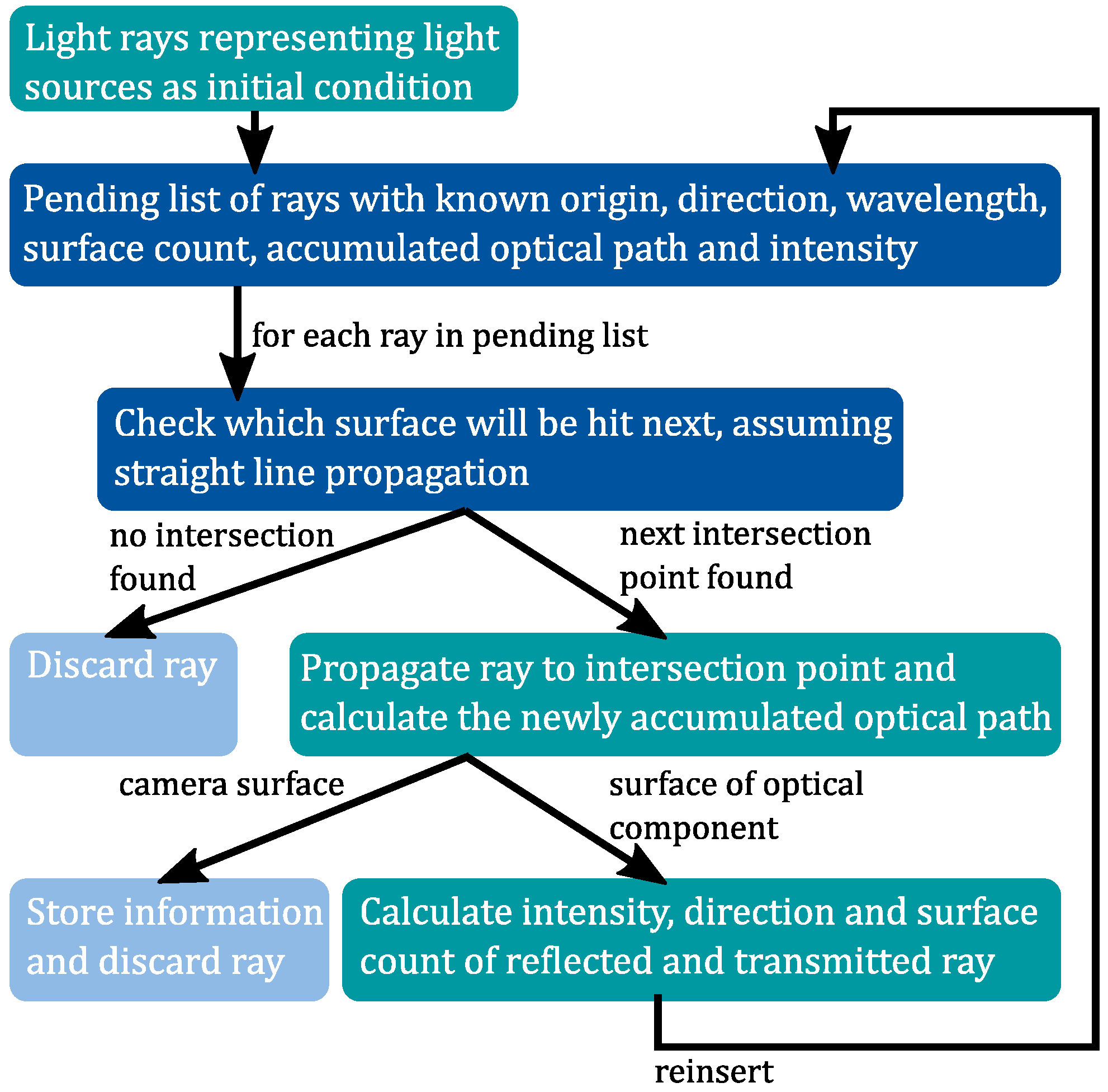
Origin, direction, intensity, and wavelength of the virtual light sources represent the initial conditions for the implemented raytracing procedure (Appendix B). When a ray intersects with a surface, it is split into a reflected and transmitted part with relative intensities according to the reflectance and transmittance coefficients (Equations (13) and (14)) [29]. The two parts are regarded as new rays originating from the intersection point with directions determined by the law of reflection (Equation (12)) and Snell’s law (Equation (11)), respectively. The number of surfaces $N_I$ hit by the initial ray is incremented (Equation (15)) and the accumulated optical path is passed to the subsequent rays. Hence, at an intersection point the following equations hold [30]:

$$\begin{array}{ccc}\hfill {\mathbf{t}}_{\mathrm{T}}& =\frac{n_1}{n_2}{\mathbf{t}}_{\mathrm{I}}-\left(\frac{n_1}{n_2}{\mathbf{t}}_{\mathrm{I}}·\mathbf{u}-\sqrt{1-{\left(\frac{n_1}{n_2}\right)}^2\left(1-{\left({\mathbf{t}}_{\mathrm{I}}·\mathbf{u}\right)}^2\right)}\right)\mathbf{u}\hfill & \hfill \left(11\right)\\ \hfill {\mathbf{t}}_{\mathrm{R}}& ={\mathbf{t}}_{\mathrm{I}}-2\left({\mathbf{t}}_{\mathrm{R}}·\mathbf{u}\right)\mathbf{u}\hfill & \hfill \left(12\right)\\ \hfill I_{\mathrm{T}}& =T·I_{\mathrm{I}}\hfill & \hfill \left(13\right)\\ \hfill I_{\mathrm{R}}& =R·I_{\mathrm{I}}\hfill & \hfill \left(14\right)\\ \hfill N_{\mathrm{T}}& =N_{\mathrm{R}}=N_{\mathrm{I}}+1\hfill & \hfill \left(15\right)\end{array}$$

In the above equations, $\mathbf{t}$ denotes the direction of a ray, I its intensity, and N its surface count. Vector $\mathbf{u}$ refers to the normal vector of the surface along the direction of transmittance and $n_{1,2}$ to the refractive indices on both sides in the same order. The indices I, R, and T correspond to incident, reflected, and transmitted rays, respectively. Finally, the raytracing procedure is continued with the two latter rays. Refraction and reflection are the only phenomena taken into account to determine the propagation direction and hence the mathematical model of the sensor established in Section 3 is not used as a priori information.

The formulation of a virtual machine tool can be simplified to two coordinate systems. These are a fixed system representing the machine frame, and a mobile coordinate system attached to the functional point which will be translated and rotated equivalently to the tool movement. The optical components are grouped into a stationary assembly described in the fixed coordinate system and a target assembly described in the mobile coordinate system. The virtual tool movement is described as the displacement and reorientation of the mobile coordinate system relative to the fixed one. From the perspective of raytracing, this corresponds to the generation of a new scene. Therefore, the simulation of the sensor is performed individually for each position in a virtual calibration cycle.

For the simulation of the sensor’s behaviour, it is irrelevant if the tool movement is ideal or superposed with geometric errors. Hence, the total error motion is added to the movement of the functional point before the raytracing scene is generated. For this purpose, a pre-generated map of the axes’ deviation in combination with the full-rigid-body model is used. The extension to a Monte-Carlo simulation consists of generating multiple scenes varying selected parameters according to a statistical distribution. On the computational side, all scenes are independent and the execution can be efficiently parallelized.

The virtual setup was used to validate the mathematical formulations stated in Section 3 and their according propagation of uncertainties. Moreover, systematic errors on the alignment constants $a_{CB},b_{CB},c_{CB},a_{CM},b_{CM},c_{CM}$, and $c_I$ were induced on purpose, confirming that $c_{CB}$ and $b_{CB}$ are most critical, as these constants neither cancel out when calculating error parameters of a linear axis according to ISO 230-1:2012(en) nor is their contribution to the total uncertainty budget after propagation negligible as for example for $a_{CB}$. Hence, a calibration procedure for $c_{CB}$ and $b_{CB}$ with an uncertainty ($k=1$) of approximately $1\mathsf{\mu }\mathrm{m}$ should be established. In the future, the virtual sensor will also be used to investigate the other hardware layouts introduced in Section 3 and different step diagonal machine tool calibration approaches [31].

6. Experimental Results of a Prototype Setup

According to the concept presented in Section 3, the authors implemented a prototype using the following components:

• The Premier LC laser diode (635 nm wavelength) manufactured by Global Laser and already used in Section 4 [18].
• Two Basler acA3800-10gm CMOS cameras with a pixel pitch of $1.67\mathsf{\mu }\mathrm{m}$ and a frame rate of $10\mathrm{Hz}$ [32].
• Two Thorlabs NE20A neutral density filters with a transmission of $1\%$ [33].
• A Thorlabs CCM1-BS013/M 50:50 cubic beamsplitter with an edge length of $d_{beamsplitter}=25.4\mathrm{mm}$ and anti-reflective coating [34].
• A Thorlabs BSW30 50:50 semi-translucent mirror with a thickness of $d_{mirror}=8\mathrm{mm}$ and an anti-reflective back side [35].
• An IDS 3010 fibre-based interferometer manufactured by Attocube, operated at a wavelength of $1530\mathrm{nm}$ with an uncertainty ($k=2$) of $1\mathsf{\mu }\mathrm{m}/\mathrm{m}$ over a $5\mathrm{m}$ displacement range with a bandwith up to $25\mathrm{MHz}$ [36,37].
• The inclinometer was omitted for the prototype as it is expected to operate independently. Thus, there is no experimental data for the roll error motion.

The entire setup is depicted in Figure 4. For validation purposes, the setup was mounted to a three-axis kinematic of gantry type without a built-in linear encoder, in parallel with a calibrated XD-Laser Precision from API [10] as a reference instrument while fixing both measurement heads on a common metal bar. The data was captured at equidistant stationary points along the gantry axis. The error parameters measured by the XD-Laser Precision instrument were corrected for the Abbe error introduced by the offset between both systems. The alignment constants $a_{CB},b_{CB},c_{CB},a_{CM},b_{CM},c_{CM}$ and $c_I$ were calculated based on the dimensions of the component mountings used and the technical drawings provided by the cameras’ manufacturer. 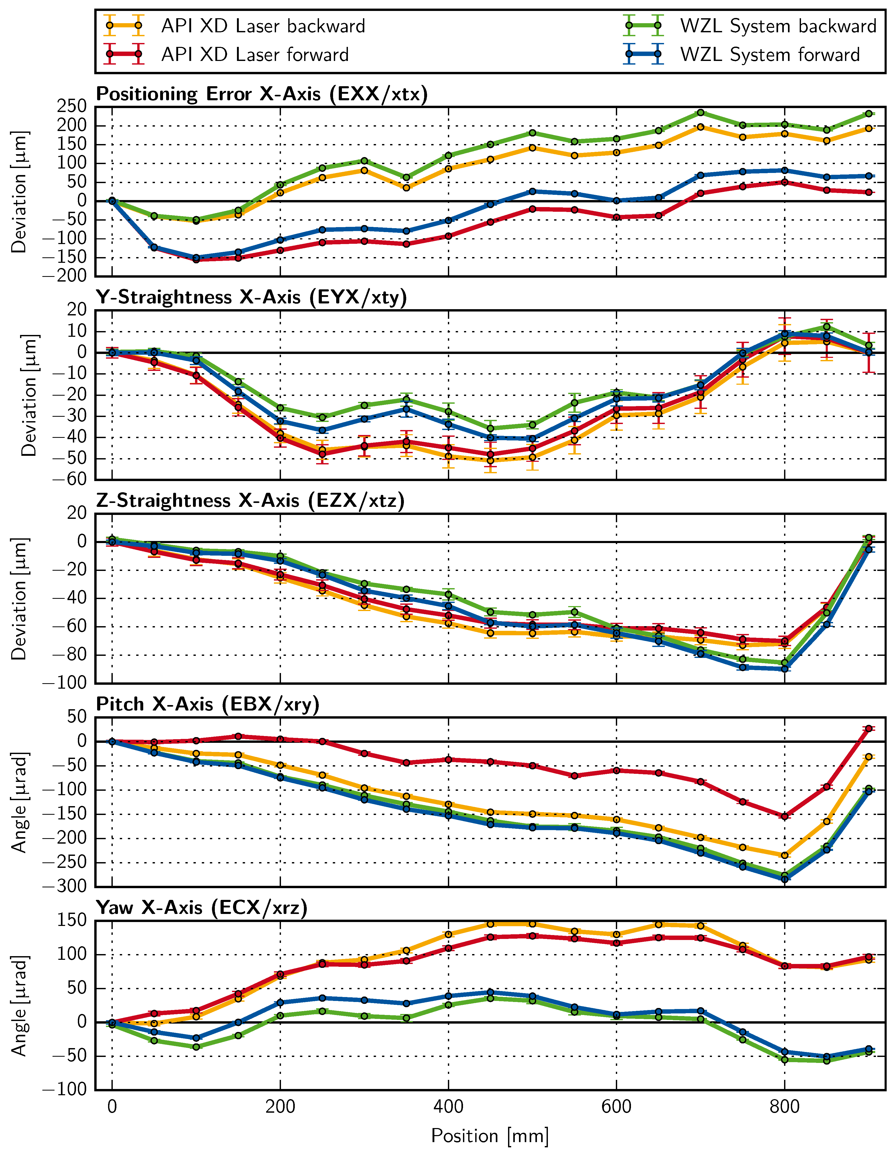Figure 5 shows a direct comparison of positioning (EXX), straightness (EYX, EZX), yaw (EAX), and pitch (EBX) error motions named adhering to ISO 230-1:2012(en) [2]. The error motions EXX along the axis itself are in very good agreement. The remaining differences are assumed to be due to different data from both interferometers’ environmental sensor units entering the refractive index calculation. Moreover, the straightness error motions EYX and EZX agree very well bearing in mind the uncertainty budget and potential systematic errors arising from the Abbe error correction based on the data for the angular error motions EAX, EBX and ECX. The latter two unveil systematic differences between the measurements of the newly developed system and the API XD-Laser reference. In the case of EBX, an offset of up to $200\mathsf{\mu }\mathrm{rad}$ between the API XD-Laser’s measurements in forward and backward direction can be observed, which is not present in the data captured with the self developed sensor during the same calibration cycle of the kinematic. The authors assume that this behaviour is an artefact of the API instrument. The correlation, i.e. the qualitative similarity of both datasets, can still be regarded as very high. The same holds for the ECX error motion, although here the offset is attributed to a systematic error on the alignment constant $c_{CB}$, as similar behaviour has been observed during the simulated experiments in Section 5. An improved calibration procedure for the alignment constants is subject to current research within the project.

The response time of the system, which will determine degree of integration into the machine tool’s control loop, has not been addressed yet. For the prototype the analysis of the beam profiles captured by the two cameras is carried out on an ordinary computer after transmitting the entire image through the Ethernet. This approach was chosen to first ensure the correct functionality of the sensor setup before optimizing latency and measurement rate. The latter will be limited by the acquisition rate of the camera chip used in the final setup, as the evaluation of the beam profiles can be shifted onto an field-programmable gate array (FPGA) directly connected to the imaging sensor.

7. Conclusions and Outlook

The presented concept of structure integrated sensors is suited to improving the time-efficiency of three-axis Cartesian machine tool calibration compared to current manual methods and enhances the potential of automation. The carried-out investigations sustain that laser diodes in combination with CCD/CMOS cameras, fibre-based interferometers, and inclinometers are eligible for a compact sensor setup that measures all six error motions of a rigid body component. Competitive measurements between the implemented prototype and a commercial machine tool calibration interferometer show good agreement with few remaining systematic errors, which will be further investigated by the authors.

At the same time, the sensor setup will be integrated into a machine tool of a gantry type serving as a permanent test carrier. Moreover, the machine tool’s control has been adapted to process and compensate the error parameters measured by the sensor on-line automatically. As a consequence, the influence of vibrations and short-term environmental fluctuations within the machine tool on the stability of the measurement process have to be reevaluated. Once the development of the single-axis prototype is completed, it will be extended to the other axes of the machine tool.