Pearl-Chain Formation of Discontinuous Carbon Fiber under an Electrical Field

Abstract

The purpose of this paper is to develop a theoretical derivation on aligning discontinuous carbon fiber with an applied electric field, and prove the theory with experiment. A principle with regard to the occurrence of carbon fiber alignment is presented after an introduction of the electromechanical quantities of dielectrics. Based on this principle, an estimation of the polarizability tensor is employed to calculate the required electric field to achieve fiber alignment in liquid solution (e.g., water, resin, etc.). Individual carbon fiber is modeled as a polarizable dielectric cylinder in liquid resin and its motion under direct current (DC) electrical field is decomposed into a polarization effect and rotation effect. A value of 20.12 V/mm is required to align short carbon fibers (0.15 mm) long in liquid resin and is experimentally validated. Finally, an expression to include weight percentage as a means of controlling pearl-chain formation is derived to change the composite’s electrical conductivity.

1. Introduction

Carbon fibers (CF) possess excellent material properties such as high stiffness, high tensile strength, and low thermal expansion, and they have been used extensively in various applications, especially as reinforcement to form composites [1,2,3,4,5]. Continuous carbon fiber has the ability to stop crack formations at fiber/matrix interfaces [6]. In this paper, we demonstrate that discontinuous carbon fiber can be aligned under a direct current (DC) electrical field in a liquid solution (e.g., water, resin, etc.). By adjusting electrical intensity, fiber geometry, and fabrication temperature, it is practical to use a small electrical intensity to align discontinuous carbon fibers. When the carbon fiber strands are connected through a pearl-chain formation, it allows current to flow through and thus, increases the overall electrical conductivity of the resulting composite (when making polymer or ceramic composites via resin solidification or pyrolysis step).

It has been shown that the mechanical strength and electrical properties of carbon fibers are superior along the axial direction than normal to it [7]. Thus, alignment of short carbon fiber is of great importance, e.g., carbon nanotubes (CNTs) have the same anisotropic properties and have been widely investigated in composite study [8,9]. There have been different processes documented in literature in order to align short fibers (or CNTs), e.g., magnetic field [10,11,12,13], gas flow [14,15], shear flow [2,16,17,18], mechanical shear press [2,19,20], mechanical stretch [21], and electrical field [22,23,24,25,26,27,28]. While mechanical methods of alignment allow production of large size samples, it is still costly and has specific requirements for sample preparation [22]. Magnetic alignment has been used to align short carbon fibers, however, due to the low magnetic sustainability of short carbon fiber, high intensity fields are required, which consume too much energy and increases the processing cost [13].

Electrical field alignment is presented in this paper given its low experimental setup requirement, duration to align, and it is environmentally friendly. Such methods are suitable for various types of dielectric fibers, e.g., carbon fiber, carbon nanotube, SiO₂ fiber, SiC fiber, Al₂O₃ fiber, etc. In this paper, carbon fiber is a typical anisotropic dielectric material and is used as an example for theoretical derivation and experimental validation.

The main contribution of this paper is the theoretical derivation of a minimum electrical field intensity required to align short carbon fiber in a liquid precursor and is experimentally validated. Pearl-chain formation is derived based on the weight ratio of carbon fiber to liquid resin. Under an electrical field, discontinuous carbon fiber undergoes both rotational and translational motions. The minimum weight fraction of short carbon fibers is calculated, which acts as the threshold value to form pearl-chain phenomenon in a liquid precursor.

Table 1. Nomenclature for Variables.

Parameter	Symbol	Parameter	Symbol
Dipole Moment	$\overrightarrow{p}$	Exterior Electric Field	$\overrightarrow{E_{ext}}$
Polarizability	$\alpha$	Electric Field Amplitude	A
Electrical Field	$\overrightarrow{E}$	Final Work	W
Radius of sphere	a	Boltzmann’s Constant	$K_B$
Vacuum Permittivity	${ϵ}_0$	Absolute Temperature	T
Dielectric Constant(Resin)	$k_1$	Dielectrophoretic Force	$F_{DEP}$
Dielectric Constant(fiber)	$k_2$	Conductivity of Carbon Fiber	${\sigma }_1$
Polarization Forces	$F_{\pm }$	Conductivity of liquid Resin	${\sigma }_2$
Charge of Carbon Fiber	q	Local Electric Field	$\overrightarrow{E_{loc}}$
Torque	$\tau$	Total Dipole	$p_0$
Electric Potential	$U(\theta )$	Distance between Carbon Fibers	d
Electric Potential(initial state)	U(0)	Potential of Carbon Fiber Pairs	$U_l$
Dipole Work	$W_1$	Work to bring Carbon Fibers together	$W_{DEP}$
Aligning Dipole Work	$W_2$	Density Ratio	v
Radius of Fiber	R	Density of Carbon Fiber	${\rho }_1$
Length	l	Density of Liquid Resin	${\rho }_2$
Inner Electrical Field	$\overrightarrow{E_{inn}}$	Number of Fibers	n
Radius of Spacing between Carbon Fiber Pairs	$r_{avg}$

contains the nomenclature for the parameter names and symbols used throughout the paper.

2. Theoretical Derivation for Calculating Required Minimum Electrical Field for Discontinuous Carbon Fiber Alignment

This section describes the theoretical derivation for finding the required electrical field intensities to align discontinuous carbon fiber in a liquid precursor matrix. To calculate the minimum required electrical field, the energy required in the alignment process is broken into two parts: (1) producing the dipole along the carbon fiber and (2) aligning the carbon fiber along the direction of the electrical field.

2.1. Producing Dipole along the Carbon Fiber

A neutral particle will have symmetric arrangements of electrons in their electron clouds that may be distorted when influenced by an electrical field. The polarization responds to the field as an instant torque on the positive and negative charges of its atom. The distribution of electrons are moved by an external field. The ease of distortion/motion is defined as the polarizability and is a three dimensional tensor. Polarizability is given by [29]:

$$\overrightarrow{p}=\alpha \overrightarrow{E},$$

(1)

where the dipole moment $\overrightarrow{p}$ is a function of the materials polarizability $\alpha$ and the given electrical field $\overrightarrow{E}$. Intuitively, a larger electrical field produces a greater dipole along the surface of the carbon fiber.

For a dielectric sphere in a given electrical field , the dipole produced can be expressed as [29]

$$\overrightarrow{p}=4\pi a^3{\epsilon }_0{k}_1(\frac{k_2-k_1}{k_2+2k_1})\overrightarrow{E},$$

(2)

where a is the radius of the sphere, ${\epsilon }_0$ is the dielectric constant of vacuum and is equal to 8.85 × 10⁻¹² F/m, $k_1$ is the dielectric constant of liquid resin, and $k_2$ is the dielectric constant of the dielectric sphere.

When a discontinuous carbon fiber is submerged into an electrical field, the carbon fiber will be polarized. This polarization results from a pair of forces $F_{\pm }$, acting on the opposite ends of fiber, as shown in Figure 1. This creates the dipole along the fiber length direction. If the carbon fiber is assigned a charge of 2q and the length of the carbon fiber is 2d, the norm of the force pair exerted at a distance of s from the center can be represented by

$$F_{\pm }=\frac{s}{d}\mathit{qE},$$

(3)

where E is the provided electrical field intensity.

Integrating the force along the axial direction pulls out the electrical charges to the tip of the fiber, the total work required to create a dipole can be calculated as

$$W_1={\int }_0^d{F}_{\pm }ds=\frac{\mathit{qE}}{d}{\int }_0^d\mathit{sds}=\frac{1}{2}\mathit{qEd}=\frac{1}{2}\mathit{pE},$$

(4)

where $W_1$ is the total work required to produce a dipole along the length of an individual carbon fiber, and therefore the charges +q and −q are pulled to the tip of the fiber on each end.

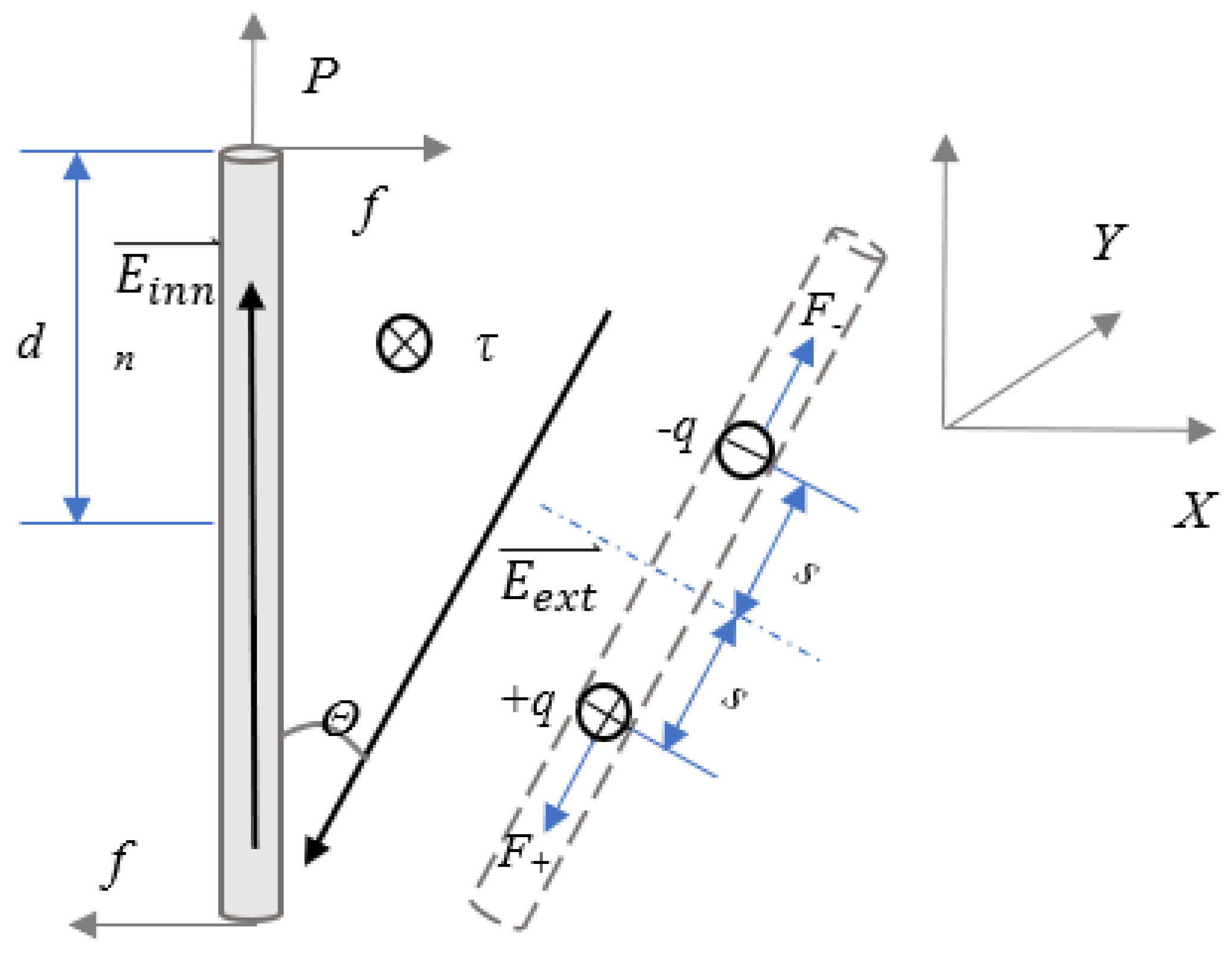
2.2. Aligning the Fiber along the Direction of the Electrical Field

In order to align a fiber along the direction of the electrical field, the torque required to rotate the carbon fiber and the angle of rotation must be calculated. is a pair of forces f at a distance of 2d will cause the carbon fiber to rotate and then align to the electrical field direction (as the dashed line position shown in Figure 1, which is parallel to the direction of external electrical field $\overrightarrow{E_{ext}}$). In a three-dimensional space, the norm of the torque equals the cross-product of the dipole moment $\overrightarrow{p}$ and the electrical field $\overrightarrow{E}$ , which can be calculated as

$$\left|\tau \right|=|\overrightarrow{p}\times \overrightarrow{E}|=\mathit{pE}sin\theta .$$

(5)

If an arbitrary angle $\theta$ is introduced as a starting angle for the carbon fiber, then integrating the torque with respect to the angle results in the work required to align the carbon fiber as

$$W_2={\int }_{\theta }^0\tau (\theta )d\theta =-\mathit{pE}+\mathit{pE}cos\theta =U(0)-U(\theta ),$$

(6)

where U($\theta$) is the electrical potential of the field exerted on the carbon fiber at the starting angle of $\theta$, and U(0) is the initial state. When setting U(0) to zero, the work required to align the fiber can be simplified as:

$$U(\theta )=-\mathit{pE}cos\theta .$$

(7)

The value when $\theta =\frac{\pi }{2}$ is exactly the maximum torque required to align the carbon fiber when the initial direction of the carbon fiber is perpendicular to the applied electrical field.

2.3. Total Work Required for Discontinuous Carbon Fiber Alignment

Now that the work required for producing a dipole and aligning the fiber have been calculated, the total work required for alignment can be found by adding $W_1$ and $W_2$. The total work for alignment can be calculated by

$$W=W_1+W_2=-\mathit{pE}+\mathit{pE}cos(\frac{\pi }{2})+\frac{1}{2}\mathit{pE}=-\frac{1}{2}\mathit{pE}.$$

(8)

After substituting the dipole moment $\overrightarrow{p}$ into the total work, the amount of total work required can be represented by

$$W=-2\pi a^3{\epsilon }_0{k}_1{(\frac{k_2-k_1}{k_2+2k_1}E)}^2,$$

(9)

where a is the radius of a spherical particle. For carbon fiber, a is replaced by the fiber’s radius of gyration [6,30]:

$$a=(\frac{R^2}{2}+{\frac{l^2}{12}}^{1/2})\approx {(\frac{l^2}{12})}^{1/2},$$

(10)

where l is the length of the carbon fiber and R is the radius of the carbon fiber.

For a small sphere of an ideal dielectric entering a uniform field, an inner electric field is created along the carbon fiber. If a fluid medium has a uniform electrical field and a neutral spherical particle is submitted into this field, then the uniform field is distorted by the sphere to give rise to an internal field interior to the spheres boundaries [29]. Since a discontinuous carbon fiber can be viewed as a tiny capacitor, the local electric field generated internally should not be neglected. With the defined inner electrical field $\overrightarrow{E_{inn}}$ and exterior field $\overrightarrow{E_{ext}}$, the electrical fields can be calculated as [31]:

$$\overrightarrow{E}=\overrightarrow{E_{\mathit{ext}}}-\overrightarrow{E_{\mathit{inn}}},$$

(11)

$$\overrightarrow{E_{\mathit{inn}}}=\frac{3{\epsilon }_1}{{\epsilon }_2+2{\epsilon }_1}\overrightarrow{E_{\mathit{ext}}},$$

(12)

$$\overrightarrow{E}=\frac{{\epsilon }_2-{\epsilon }_1}{{\epsilon }_2+2{\epsilon }_1}\overrightarrow{E_{\mathit{ext}}},$$

(13)

where ${\epsilon }_1$ and ${\epsilon }_2$ are equal to ${\epsilon }_0\ast k_1$ and ${\epsilon }_0\ast k_2$, respectively. When a sinusoidal electrical field is applied, the scalar value of the electric field can be calculated as

$$E^2=\frac{{\int }_0^T{(Asin(\omega t))}^2\mathit{dt}}{{\int }_0^T\mathit{dt}}=\frac{A^2}{2},$$

(14)

where A is the amplitude of the sinusoidal electric field strength. Combining (9)–(11) and (14), the final work for carbon fiber alignment can be found by

$$W=-2\pi {(\frac{l^2}{12})}^{3/2}{\epsilon }_0{k}_1(\frac{k_2-k_1}{k_2+2k_1})\frac{A^2}{2}.$$

(15)

Thus the static mechanical analysis is complete and the amplitude, A, of the required external electrical field can be obtained.

2.4. Summary on Minimum Required Electrical Field for Alignment

The required electrical field to align carbon fiber is dependent on temperature and can be calculated by [32]

$$\left|W\right|\ge K_{B}T,$$

(16)

where $K_B$ is Boltzmann’s constant (1.38 × 10⁻²³ JK⁻¹), and T is the absolute temperature (K) of the environment.

3. Simulation Result on Required Minimum Electrical Field

From the above analysis, several factors can be adjusted in order to minimize the required electrical field strength to align the carbon fiber. In summary there are five parameters that will affect the minimum electrical field intensity.

(1)

Length of the discontinuous fibers: the longer the fiber, the smaller the required electrical field intensity (E).

(2)

Diameter of the discontinuous fibers: this factor usually can be ignored with a large aspect-ratio (>10). If it is considered, the smaller the diameter, the smaller the required E.

(3)

Combined effect-dielectric constant of the discontinuous fibers ($K_2$) and dielectric constant of the liquid resin ($K_4$): the larger the $K_1{(K_2-K_1)}^2/{(K_2+2K_1)}^2$ value, the smaller the required E.

(4)

Fabrication temperature: the lower the temperature, the smaller the required E.

(5)

Viscosity of the liquid resin: Viscosity value does not affect the required E. However, the smaller the viscosity, the shorter time required to align the fiber. For a high viscous material, the time for alignment will still be within minutes.

By changing these five parameters it is possible to tailor the environment to allow for a smaller electrical field intensity to align the carbon fiber.

During simulation, as listed in

Table 2. Input/Output for simulation.

	Parameter	Symbol	Value	Units
Input	Length	l	0.15	mm
	Radius of Fiber	R	8	µm
	Dielectric Constant(fiber)	$k_1$	2.85
	Dielectric Constant(Resin)	$k_2$	3.45
	Vacuum Permittivity	${ϵ}_0$	8.85 × 10−12	F/m
Output	Electric Field Amplitude	A	20.12	V/mm

, the length of carbon fiber l is assumed to be 0.15 mm (on average), and the radius of carbon fiber is 8 µm. The dielectric constant of carbon fiber is chosen as $k_2=2.85$. The dielectric constant of liquid resin (the ceramic precursor in this research) is $k_1=3.45$. The vacuum permittivity, ${ϵ}_0$ is taken as 8.85 × 10⁻¹² F/m. The value of the required electric field to align the discontinuous carbon fiber at room temperature is calculated to be 20.12 V/mm, which means that to align carbon fiber in a 1 mm width reservoir, a 20.12 V supply is needed.

From the theoretical derivation in the previous section, it can be seen that the larger the aspect ratio of carbon fiber, the smaller electrical field one needs to align the carbon fiber. Simulations were ran in MATLAB and tabulated in

Table 3. Required electrical field for a mat-shaped sample (Simulation result).

Fiber Diameter = 16 µm
Required Electrical Field (V)		Fabrication Temperature	Fabrication Temperature	Fabrication Temperature
		25 °C	75 °C	100 °C
		16 µm	16 µm	16 µm
Fiber Length	10 mm	11.26	11.71	11.91
	50 mm	1.01	1.05	1.07

, which shows the required electrical field intensities to align carbon fiber in a mat-shaped sample (a standard 12 inch × 12 inch pre-preg sample size). It is noticed that for standard fibers with 16 µm diameter and 10 mm length in room temperature, only 11.26 V is needed to align the short carbon fibers, which is quite feasible to achieve.

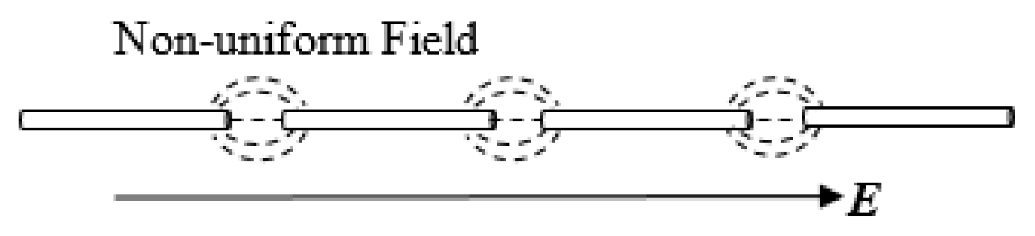
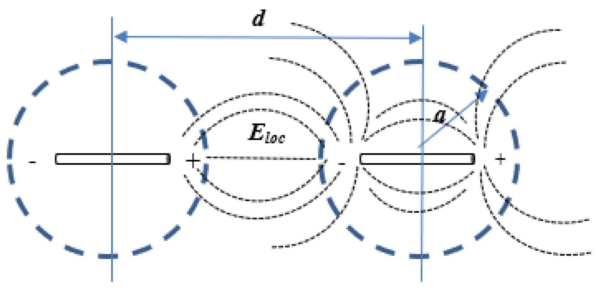
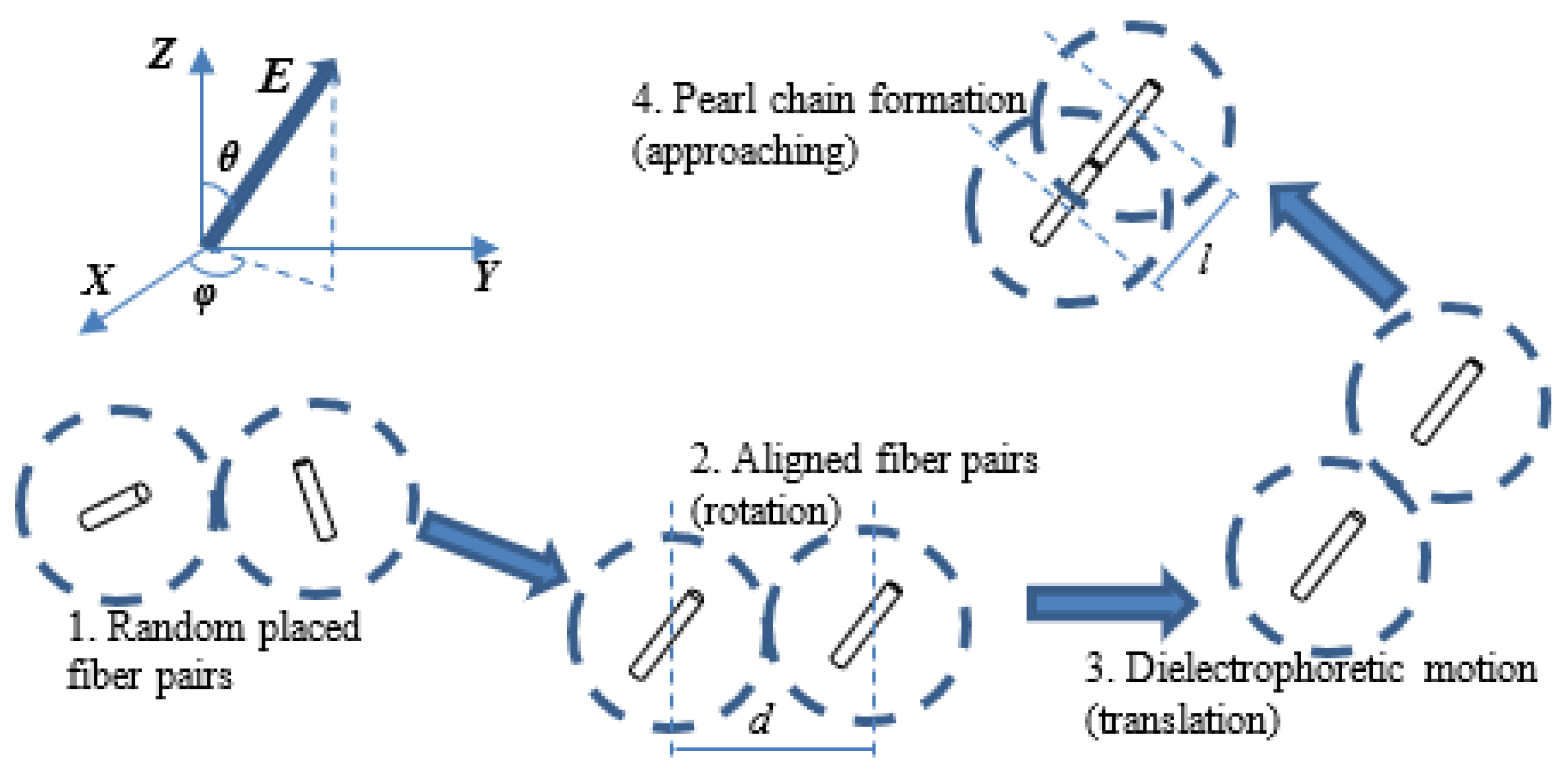
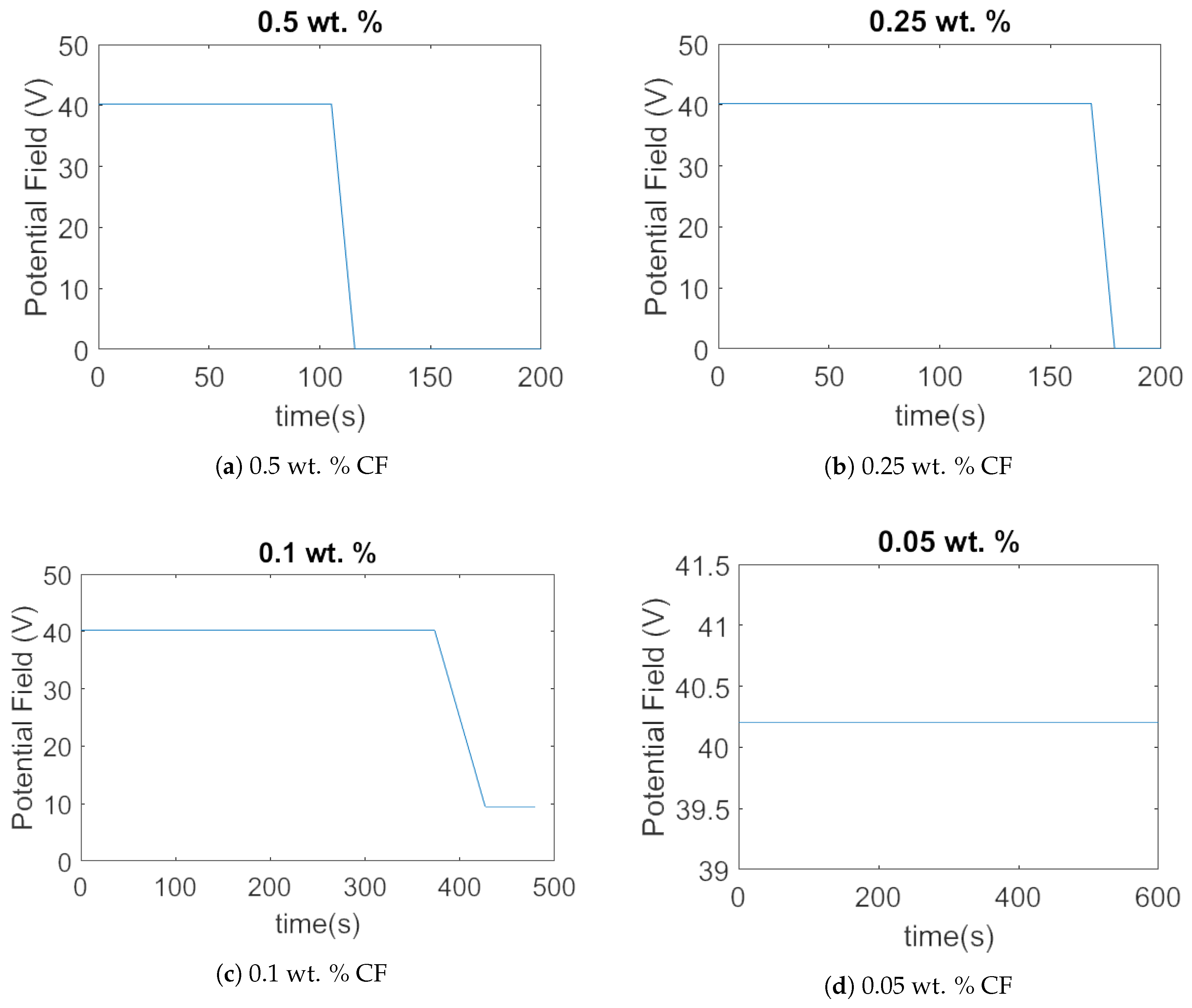
4. Pearl-Chain Formation

This section details an addition to the previous model by including a weight percentage so that pearl-chain formation (head-to-toe phenomena) can be controlled in order to change the composites physical properties. While pearl-chain formation creates micro electrical networks within the dielectric resin, weak points can be formed due to the formation of carbon fiber chains and affect the resultant overall electrical resistivity.

In the previous model, the discontinuous carbon fibers were assumed to align in a uniform electric field. It is known that when an electrical field is applied to a group of neutral particles, bunching will occur [29]. This effect can be observed after alignment by the creation of chain-like structures formed along the applied electrical field. These-chain like structures are referred to as pearl-chain formation (head-to-toe phenomena) and can be explained by self-induced electric fields created by each carbon fiber strand. When neutral particles have a higher polarizability than the surrounding medium, they distort the field created in the medium. Each individual particle then experiences a non-uniform electric field near each carbon fiber strand. This produces a dielectrophoretic force at both sides of the carbon fiber which can be seen in Figure 2 and can be calculated by [33]

$$F_{\mathit{DEP}}=\frac{\pi R^{2}l}{2}{\epsilon }_1\frac{{\sigma }_2-{\sigma }_1}{{\sigma }_1}\nabla E^2$$

(17)

where ${\sigma }_1$ and ${\sigma }_2$ are the conductivity of carbon fiber and liquid resin respectively, and E is the magnitude of the nonuniform electric field. It can be seen that the dielectrophoretic force is dependent on the gradient of the nonuniform electric field. Since the carbon fiber strands are already polarized by the external field, they are aligned in parallel to the electric field. Then, as the carbon fiber strands develop a dielectrophoretic force, they begin to move towards a higher intensity electric field produced by each individual fiber. These higher intensity fields cause the carbon fiber strands to move towards each other, forming chain-like formations which can be seen in the experiment after alignment is completed. This effect is referred to as mutual dielectrophoresis [29] and is illustrated in Figure 2.

Pearl-chain formation creates micro electrical networks when the carbon fibers come in contact through pearl-chain phenomena. Current flows through these carbon fiber networks after alignment. If there are enough carbon fibers in the liquid resin then bunching will occur creating the electrical networks inside the precursor.

In Figure 3a diagram of carbon fibers and their induced electrical fields can be seen, where the carbon fiber pairs are subject to both the external uniform field as well as the local induced non-uniform field created by the carbon fiber pairs at a distance d from each other.

The dipole created by the external field has already been calculated in (2). The induced dipole created by the local field can be calculated by making an assumption that the carbon fibers can be modeled as large circular, polarizable particles. This assumption makes the analysis of the induced dipole similar to the analysis of the dipole created by the external field. Based on the same process, the induced dipole caused by the local field can be calculated by [34]

$$\overrightarrow{p_1}=4\pi a^3{\epsilon }_0{k}_1(\frac{k_2-k_1}{k_2+2k_1})\overrightarrow{E_{\mathit{loc}}}=\alpha \overrightarrow{E_{\mathit{loc}}},$$

(18)

where the magnitude of the local field $\overrightarrow{E_{loc}}$ at a distance d and a dipole $p_0$ can be calculated by [34]

$$E_{\mathit{loc}}=\frac{p_0}{2\pi {\epsilon }_1{d}^3}e.$$

(19)

Here the induced dipole of moment $p_1$ is added to the previous dipole created by an external field, resulting in the total dipole of each carbon fiber represented by

$$p_0=p+p_1=p+\alpha E_{\mathit{loc}}.$$

(20)

If (19) and (20) are combined then the total dipole can be calculated by

$$p_0=\frac{p_1}{1-\frac{\alpha }{2\pi {\epsilon }_1{d}^3}}.$$

(21)

In order to calculate the work that the nonuniform electric field does to bring two carbon fibers together at a distance d, it is helpful to break the motion of the carbon fiber into four separate stages represented by Figure 4:

(1) The first stage of alignment is where the carbon fiber is randomly dispersed before the uniform electric field is applied. (2) The second stage, referred to as rotation, is after the uniform electric field is applied. The carbon fiber begins to rotate and align in parallel to the external electric field. (3) During the third state, referred to as translation, induced dipoles occur on the carbon fiber due to the local nonuniform electric field about the carbon fiber. This local electric field causes induced dipoles that lead to dielectrophoretic motion. (4) Finally, during the fourth stage, referred to as approaching, the induced dipoles cause the carbon fiber pairs to attract to each other, leading to pearl-chain formation. It is assumed that the carbon fibers are spaced evenly and thus the spaces of each carbon fiber pairs are equal. If the average distance between the carbon fiber pairs is d, then the electric potential can be calculated by

$$U_d=p_0{E}_{\mathit{loc}}=\frac{p_1^2}{2\pi {\epsilon }_1{d}^3}{(\frac{1}{1-\frac{\alpha }{2\pi {\epsilon }_1{d}^3}})}^2.$$

(22)

If the force $F_{DEP}$ causes a pair of carbon fiber pairs to contact head-to-toe with a distance between the centers l, then the current potential of the carbon fiber pairs can be calculated by

$$U_l=\frac{p_1^2}{2\pi {\epsilon }_1{l}^3}{(\frac{1}{1-\frac{\alpha }{2\pi {\epsilon }_1{l}^3}})}^2,$$

(23)

which is the potential of the carbon fiber after contacting. Therefore the work done by the dielectrophoretic force $F_{DEP}$ can be calculated by

$$\begin{array}{c}{W}_{DEP}=U_l-U_d\\ =\frac{p_1^2}{2\pi {\epsilon }_1}[\frac{1}{l^3}{(\frac{1}{1-\frac{\alpha }{2\pi {\epsilon }_1{l}^3}})}^2-\frac{1}{d^3}{(\frac{1}{1-\frac{\alpha }{2\pi {\epsilon }_1{d}^3}})}^2].\end{array}$$

(24)

An inequality can be formed between the work done to bring two carbon fiber pairs together and the average translational force associated with the medium. This relation can be calculated by

$$W_{\mathit{DEP}}\le \frac{3K_{B}T}{2}.$$

(25)

Using this relation, another equality can be formed in order to calculate the least weight percentage of carbon fiber to minimize pearl-chain formation. If the mass of the polymer precursor is defined as m, and the weight percentage of carbon fiber in the resin matrix is defined as w, then the density ratio of carbon fiber and liquid resin can be calculated by

$$v=\frac{{\rho }_1}{{\rho }_2}.$$

(26)

Using (26), the number of fibers n inside the liquid resin can be found by combining (27) and (28).

$$n=\frac{\mathit{mw}}{{\rho }_1\pi R^{2}l}.$$

(27)

$$V=\frac{m}{{\rho }_2}=\frac{4}{3}n\pi r_{\mathit{avg}}^3.$$

(28)

Thus if each particle takes a space of a sphere with an average radius of $r_{avg}$ and are ideally dispersed in the solvent, then the $r_{avg}$ can be calculated by [35]

$$r_{\mathit{avg}}={(\frac{3v}{4w}{R}^{2}l)}^{1/3}.$$

(29)

An inequality can be formed using (25) and after making a substitution $2\times r_{avg}=d$, the following inequality can be derived

$$\begin{array}{c}\frac{{\alpha }^2}{24\pi {\epsilon }_1^{2}v{R}^{2}l}w+6v{R}^{2}l\frac{1}{w}\le \hfill \\ \frac{1}{l^2{(1-\frac{\alpha }{2\pi {\epsilon }_1{l}^3})}^2-\frac{3K_{B}T\pi {\epsilon }_1}{p_1^2}}+\frac{\alpha }{\pi {\epsilon }_1}.\hfill \end{array}$$

(30)

Equation (30) is a $k_{1}w+\frac{k_2}{w}\le C$ inequality and provides an approximate evaluation that can decide the least amount weight percentage of carbon fiber, w, to minimize pearl-chain formation.

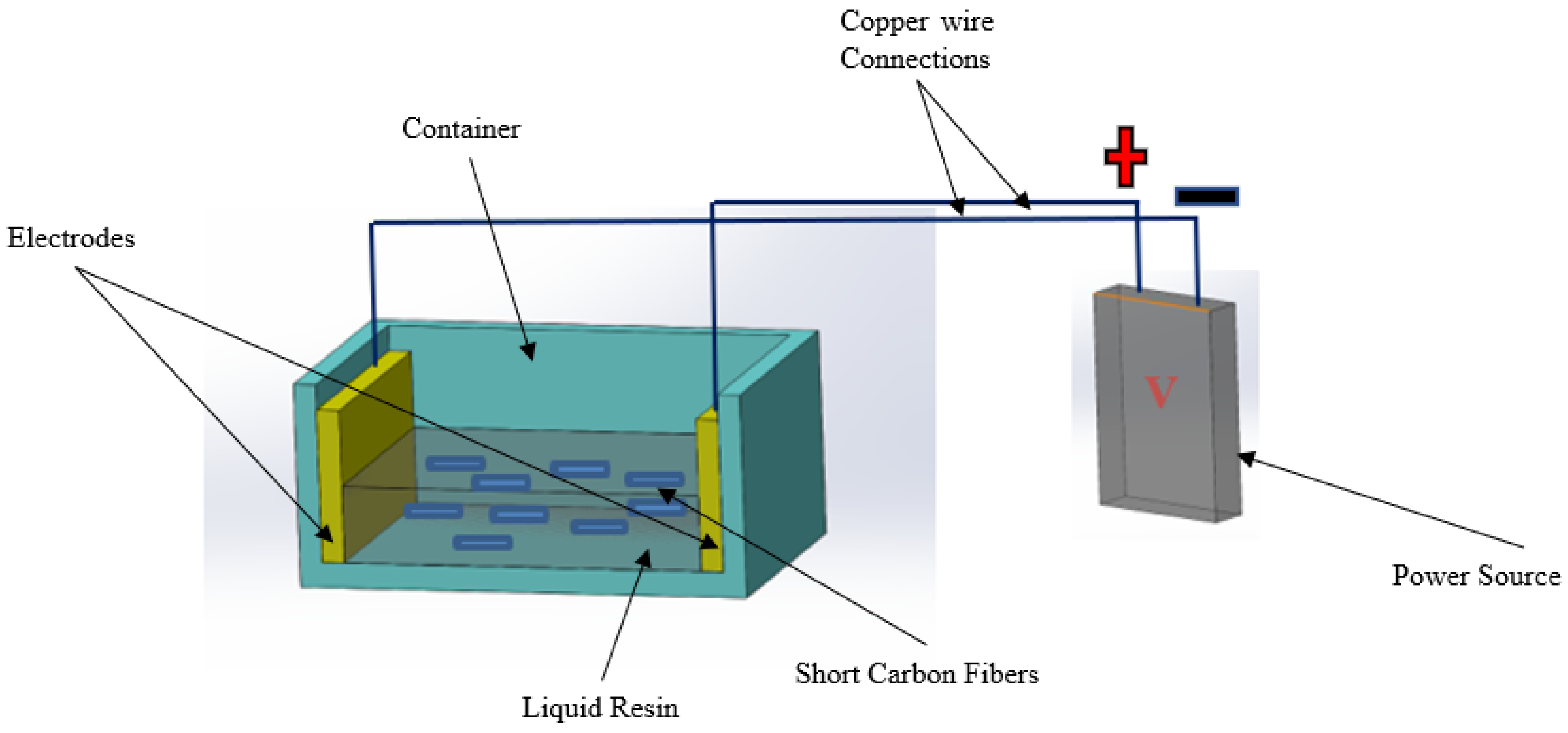
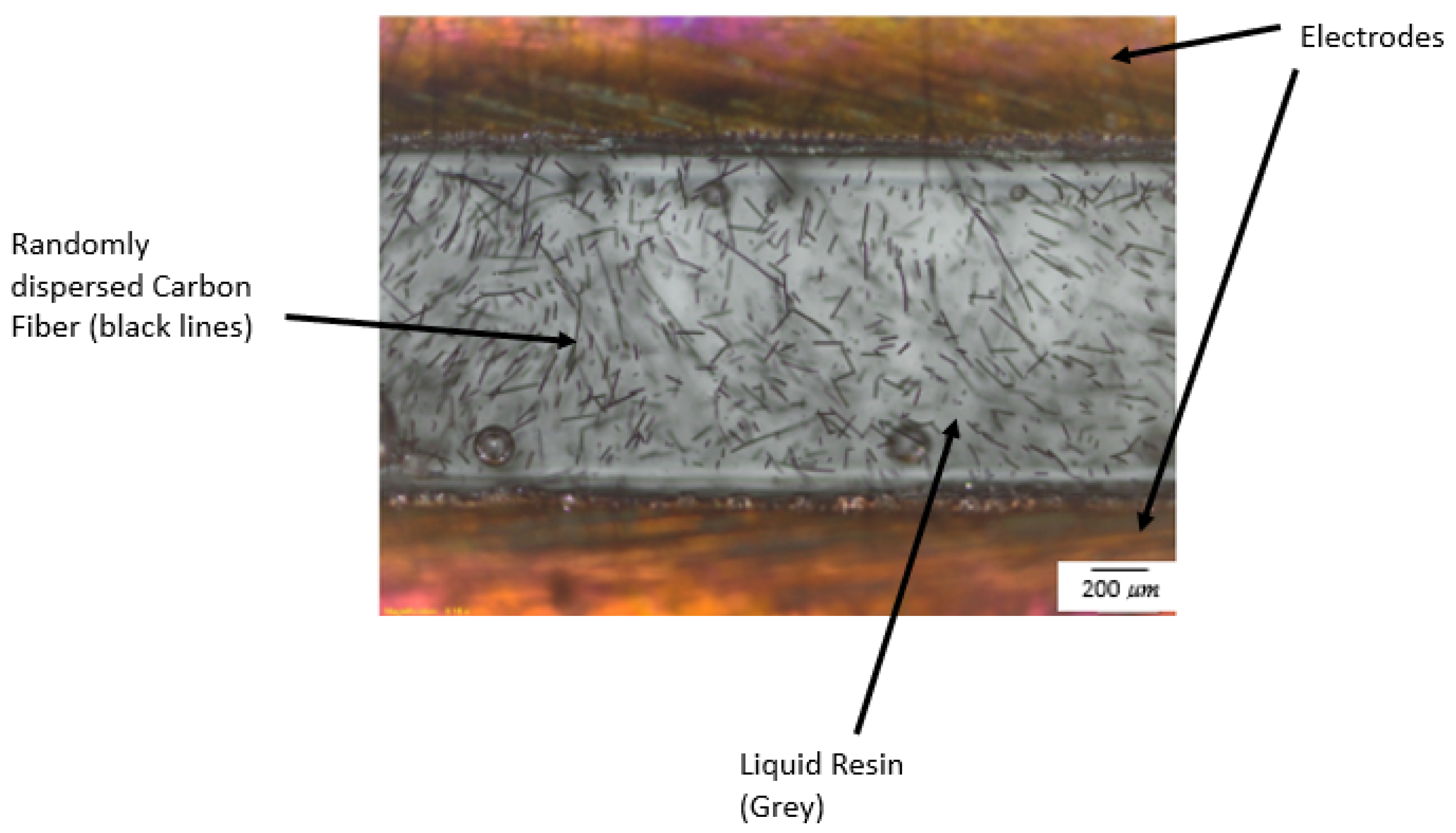
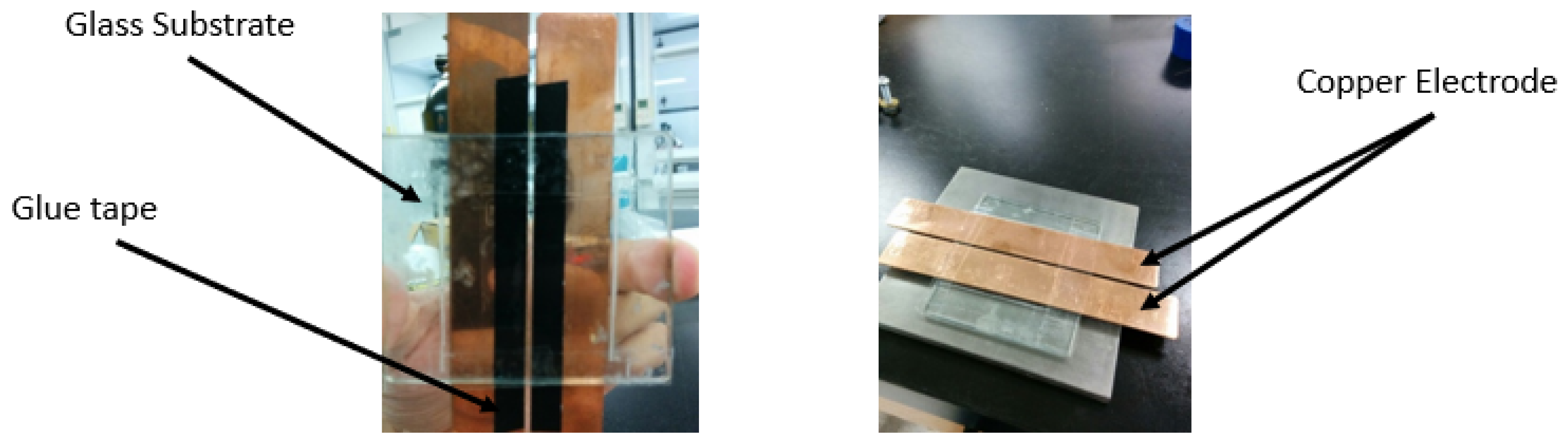
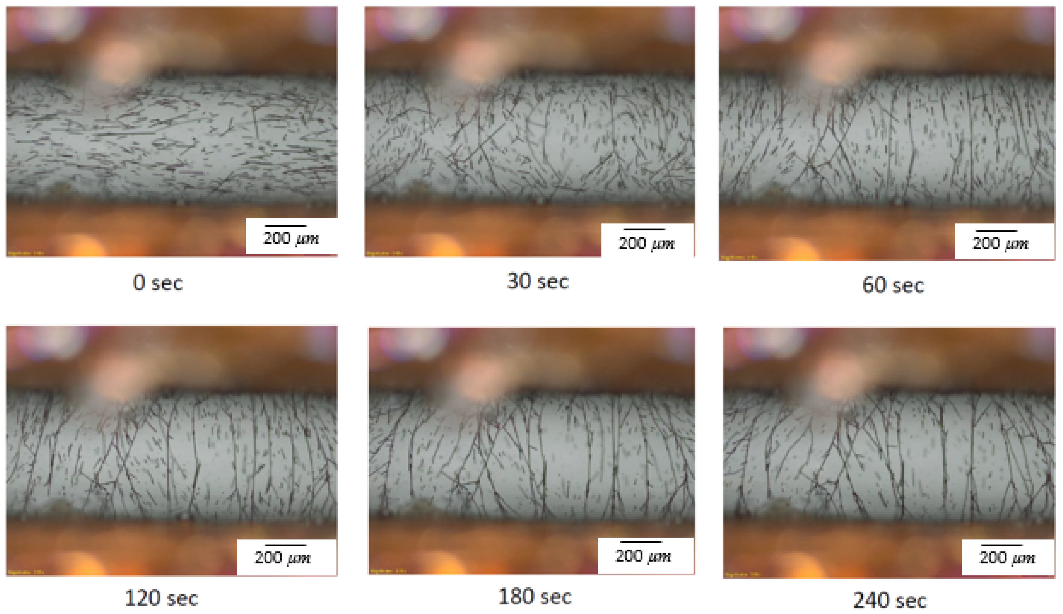
5. Experimental Setup and Result

This section details the experimental setup for carbon fiber alignment and the specifications of pearl-chain formation. This section also includes the experiment parameters used.

The experimental setup is shown in Figure 5, where the fibers and liquid solution (resin, water, etc.) are mixed in a prescribed proportion. Voltage is applied on each side of the suspension through two metal electrodes, until fibers are thoroughly aligned. Ultraviolet (UV) light or a heat source can be applied to cure the precursor into solid state. In our experiment, the liquid resin is Kion^® (Huntingdon Valley, PA, USA) Ceraset polysilazane, which is a liquid thermosetting resin containing repeat units of silicon and nitrogen atoms bonded in an alternating sequence. Polysilazane is versatile with a low viscosity of 80 cps at room temperature [36]. The short carbon fibers are mixed into the liquid resin and submitted to an electrical field. The electrical field is applied and held constant until the fibers are thoroughly aligned.

Two parallel copper electrodes were used in this experiment in order to apply the electrical field. In order to form the mixture tank, copper electrodes were attached to a glass substrate using glue tape. Glue tape was used to envelope the parallel electrodes and prevent contact (and electro-chemical reaction) between the liquid resin and the electrodes. The spacing between the electrodes is 2 mm. The electrodes and glass substrate can be seen in Figure 6.

To create the electrical fields applied to the electrodes, one digital power supply (30 V) and a high voltage amplifier (0–1000 V) were used. The amplifier has a proportional input-output and was hooked up to the power supply.

The short carbon fiber and polysilazane mixture contained 0.5 wt % short fiber. The carbon fiber was initially randomly dispersed in the liquid resin through mechanical stirring and supersonic vibrational homogenization. After dispersing the carbon fiber, the sample was placed under an optical microscope to show the random dispersion of the short carbon fiber. The randomly dispersed carbon fiber in the liquid resin can be seen in Figure 7.

A sample of the short carbon fiber and liquid resin was then placed along the 2 mm between electrodes and placed under an optical microscope for real time observation. After the carbon fiber was randomly dispersed inside of the liquid resin, an electrical field was applied to the electrodes. The fibers began to rotate instantaneously as soon as the electrical field is applied. As expected, the individual carbon fiber began to rotate and align parallel to the electrical field. The carbon fiber alignment was captured in a timed sequence using an optical microscope at 5× magnification. The entire alignment process occurred within 2 min. The alignment process was recorded in time sequence: 0 s, 30 s, 60 s, 120 s, 180 s and 240 s, as shown in Figure 8. Within the first 30 s of experimentation it can be seen that the electrical field exerts a force on the carbon fiber that causes the carbon fiber to begin to rotate. After the carbon fibers aligned parallel to the electrical field, the carbon fibers began to attract each other, causing a concatenation (pearl-chain) phenomenon. This effect can be seen after 60 s of experimentation, and continued until 120 s. After the carbon fiber formed enough networks, current was able to pass between the electrodes and caused a voltage drop between the two electrodes. This voltage drop shows the good electrical conductivity in the precursor with short carbon fibers after alignment. Thus, the experimental results agree with the simulated results for the required electric field intensity to align short carbon fibers in a liquid resin.

The same experiment was conducted with weight percentages of 0.25%, 0.1%, and 0.05% of carbon fiber (CF) solutions. The results can be seen below in Figure 9. As the weight percentage decreased, the time span before the voltage drop was increased. This was due to less pearl-chain formations occurring during alignment. The times when the voltage drop (for 0.5%, 0.1%, 0.25%) were 120 s (a), 180 s (b), 420 s (c), and the final sample (d) did not experience a voltage drop due to very few pearl-chain formations occurring.

6. Conclusions

In this paper a theoretical derivation for the required electrical field intensity was derived and proven through experimentation. The minimum electrical field was calculated to be 20.12 V/mm for an average length of carbon fiber of 0.15 mm and an average radius of 8 µm. When the electrical field was applied for a sample with a 2 mm width, alignment occurred within the first 15 s, lasting two minutes before pearl-chain formation occurred. In the experiment, short carbon fiber was selected as reinforcement in a liquid precursor. The experimental data justifies the proposed method to align discontinuous fibers in an electric field efficiently. Another theoretical contribution of this paper is the calculation for the concatenation of carbon fibers pearl-chain formation, as a function of the weight percentage. If electrical properties are needed then micro electrical networks can be created by aligning short carbon fibers and connecting the carbon fiber strands through pearl-chain formation. These carbon fiber connections allow current to flow, increasing the overall electrical conductivity of the resulting composite.

References

1. Chung, D. Carbon Fiber Composites; Elsevier: Amsterdam, The Netherlands, 2012. [Google Scholar]
2. Bradford, P.D.; Wang, X.; Zhao, H.; Maria, J.P.; Jia, Q.; Zhu, Y. A novel approach to fabricate high volume fraction nanocomposites with long aligned carbon nanotubes. Compos. Sci. Technol. 2010, 70, 1980–1985. [Google Scholar] [CrossRef]
3. Yang, J.; Dong, S.; Xu, C. Mechanical response and microstructure of 2D carbon fiber reinforced ceramic matrix composites with SiC and Ti3SiC2 fillers. Ceram. Int. 2016, 42, 3019–3027. [Google Scholar] [CrossRef]
4. Shirvanimoghaddam, K.; Hamim, S.U.; Akbari, M.K.; Fakhrhoseini, S.M.; Khayyam, H.; Pakseresht, A.H.; Ghasali, E.; Zabet, M.; Munir, K.S.; Jia, S.; et al. Carbon fiber reinforced metal matrix composites: Fabrication processes and properties. Compos. Part A Appl. Sci. Manuf. 2017, 92, 70–96. [Google Scholar] [CrossRef]
5. Naebe, M.; Shirvanimoghaddam, K. Functionally graded materials: A review of fabrication and properties. Appl. Mater. Today 2016, 5, 223–245. [Google Scholar] [CrossRef]
6. Rubinstein, M. RH Colby Polymer Physics; Oxford University Press: Oxford, UK, 2003. [Google Scholar]
7. Prasse, T.; Cavaille, J.Y.; Bauhofer, W. Electric anisotropy of carbon nanofibre/epoxy resin composites due to electric field induced alignment. Compos. Sci. Technol. 2003, 63, 1835–1841. [Google Scholar] [CrossRef]
8. Yang, J.; Downes, R.; Schrand, A.; Park, J.G.; Liang, R.; Xu, C. High electrical conductivity and anisotropy of aligned carbon nanotube nanocomposites reinforced by silicon carbonitride. Scr. Mater. 2016, 124, 21–25. [Google Scholar] [CrossRef]
9. Yang, J.; Downes, R.; Yu, Z.; Park, J.G.; Liang, R.; Xu, C. Strong and ultra-flexible polymer-derived silicon carbonitride nanocomposites by aligned carbon nanotubes. Ceram. Int. 2016, 42, 13359–13367. [Google Scholar] [CrossRef]
10. Tian, Y.; Park, J.G.; Cheng, Q.; Liang, Z.; Zhang, C.; Wang, B. The fabrication of single-walled carbon nanotube polyelectrolyte multilayer composites by layer-by-layer assembly and magnetic field assisted alignment. Nanotechnology 2009, 20, 335601. [Google Scholar] [CrossRef] [PubMed]
11. Steinert, B.W.; Dean, D.R. Magnetic field alignment and electrical properties of solution cast PET-carbon nanotube composite films. Polymer 2009, 50, 898–904. [Google Scholar] [CrossRef]
12. Byszewski, P.; Baran, M. Magnetic susceptibility of carbon nanotubes. Europhys. Lett. 1995, 31, 363. [Google Scholar] [CrossRef]
13. Camponeschi, E.; Vance, R.; Al-Haik, M.; Garmestani, H.; Tannenbaum, R. Properties of carbon nanotube-polymer composites aligned in a magnetic field. Carbon 2007, 45, 2037–2046. [Google Scholar] [CrossRef]
14. Xin, H.; Woolley, A.T. Directional orientation of carbon nanotubes on surfaces using a gas flow cell. Nano Lett. 2004, 4, 1481–1484. [Google Scholar] [CrossRef]
15. Hedberg, J.; Dong, L.; Jiao, J. Air flow technique for large scale dispersion and alignment of carbon nanotubes on various substrates. Appl. Phys. Lett. 2005, 86, 143111. [Google Scholar] [CrossRef]
16. Sulong, A.B.; Park, J. Alignment of multi-walled carbon nanotubes in a polyethylene matrix by extrusion shear flow: Mechanical properties enhancement. J. Compos. Mater. 2011, 45, 931–941. [Google Scholar] [CrossRef]
17. Dijkstra, D.J.; Cirstea, M.; Nakamura, N. The orientational behavior of multiwall carbon nanotubes in polycarbonate in simple shear flow. Rheol. Acta 2010, 49, 769–780. [Google Scholar] [CrossRef]
18. Thostenson, E.T.; Chou, T.W. Aligned multi-walled carbon nanotube-reinforced composites: Processing and mechanical characterization. J. Phys. D Appl. Phys. 2002, 35, L77. [Google Scholar] [CrossRef]
19. Wang, D.; Song, P.; Liu, C.; Wu, W.; Fan, S. Highly oriented carbon nanotube papers made of aligned carbon nanotubes. Nanotechnology 2008, 19, 075609. [Google Scholar] [CrossRef] [PubMed]
20. Yang, J.; Dong, S.; Webster, D.; Gilmore, J.; Xu, C. Characterization and Alignment of Carbon Nanofibers under Shear Force in Microchannel. J. Nanomater. 2016, 2016, 40. [Google Scholar] [CrossRef]
21. Cheng, Q.; Bao, J.; Park, J.; Liang, Z.; Zhang, C.; Wang, B. High mechanical performance composite conductor: Multi-walled carbon nanotube sheet bismaleimide nanocomposites. Adv. Funct. Mater. 2009, 19, 3219–3225. [Google Scholar] [CrossRef]
22. Martin, C.; Sandler, J.; Windle, A.; Schwarz, M.K.; Bauhofer, W.; Schulte, K.; Shaffer, M. Electric field-induced aligned multi-wall carbon nanotube networks in epoxy composites. Polymer 2005, 46, 877–886. [Google Scholar] [CrossRef]
23. Park, C.; Wilkinson, J.; Banda, S.; Ounaies, Z.; Wise, K.E.; Sauti, G.; Lillehei, P.T.; Harrison, J.S. Aligned single-wall carbon nanotube polymer composites using an electric field. J. Polym. Sci. Part B Polym. Phys. 2006, 44, 1751–1762. [Google Scholar] [CrossRef]
24. Takahashi, T.; Murayama, T.; Higuchi, A.; Awano, H.; Yonetake, K. Aligning vapor-grown carbon fibers in polydimethylsiloxane using dc electric or magnetic field. Carbon 2006, 44, 1180–1188. [Google Scholar] [CrossRef]
25. Oliva-Avilés, A.; Avilés, F.; Sosa, V.; Oliva, A.; Gamboa, F. Dynamics of carbon nanotube alignment by electric fields. Nanotechnology 2012, 23, 465710. [Google Scholar] [CrossRef] [PubMed]
26. Chen, X.; Saito, T.; Yamada, H.; Matsushige, K. Aligning single-wall carbon nanotubes with an alternating-current electric field. Appl. Phys. Lett. 2001, 78, 3714–3716. [Google Scholar] [CrossRef] [Green Version]
27. Zhu, Y.F.; Ma, C.; Zhang, W.; Zhang, R.P.; Koratkar, N.; Liang, J. Alignment of multiwalled carbon nanotubes in bulk epoxy composites via electric field. J. Appl. Phys. 2009, 105, 054319. [Google Scholar] [CrossRef]
28. Zhang, Y.; Chang, A.; Cao, J.; Wang, Q.; Kim, W.; Li, Y.; Morris, N.; Yenilmez, E.; Kong, J.; Dai, H. Electric-field-directed growth of aligned single-walled carbon nanotubes. Appl. Phys. Lett. 2001, 79, 3155–3157. [Google Scholar] [CrossRef]
29. Pohl, H.A.; Pohl, H. Dielectrophoresis: The Behavior of Neutral Matter in Nonuniform Electric Fields; Cambridge University Press: Cambridge, UK, 1978; Volume 80. [Google Scholar]
30. Hughes, M.P. AC electrokinetics: Applications for nanotechnology. Nanotechnology 2000, 11, 124. [Google Scholar] [CrossRef]
31. Fu, S.Y.; Lauke, B. Effects of fiber length and fiber orientation distributions on the tensile strength of short-fiber-reinforced polymers. Compos. Sci. Technol. 1996, 56, 1179–1190. [Google Scholar] [CrossRef]
32. Jones, T. Electromechanics of Particles; Cambridge University Press: Cambridge, UK, 1995. [Google Scholar]
33. Peng, N.; Zhang, Q.; Li, J.; Liu, N. Influences of ac electric field on the spatial distribution of carbon nanotubes formed between electrodes. J. Appl. Phys. 2006, 100, 024309. [Google Scholar] [CrossRef]
34. Von Hippel, A.R. Dielectrics and Waves; Artech House: Norwood, MA, USA, 1954. [Google Scholar]
35. Poon, W.C.; Weeks, E.R.; Royall, C.P. On measuring colloidal volume fractions. Soft Matter 2012, 8, 21–30. [Google Scholar] [CrossRef]
36. Riedel, R.; Passing, G.; Schönfelder, H.; Brook, R.J. Synthesis of dense silicon-based ceramics at low temperatures. Nature 1992, 355, 714. [Google Scholar] [CrossRef]
Figure 1. Carbon fiber positioning in an electrical field, where F ± is the pair of forces generated, q is the charge, and s is the instantaneous distance from the center of the fiber.
Jmmp 01 00022 g001
Figure 2. Pearl-chain formation caused by self-induced field.
Jmmp 01 00022 g002
Figure 3. Diagram of carbon fiber pairs with induced local electric field.
Jmmp 01 00022 g003
Figure 4. Stages of alignment for carbon fiber.
Jmmp 01 00022 g004
Figure 5. Experimental apparatus for discontinuous carbon fiber alignment.
Jmmp 01 00022 g005
Figure 6. Mixture tank made up of copper electrodes, glass substrate, and glue tape. The power source was connected to each electrode and a potential field was applied.
Jmmp 01 00022 g006
Figure 7. Randomly dispersed Carbon Fiber.
Jmmp 01 00022 g007
Figure 8. Alignment process of Carbon fiber in Polymer Precursor.
Jmmp 01 00022 g008
Figure 9. Various weight percentages: 0.5%, 0.1%, 0.25%, 0.05% of carbon fiber (CF) solutions were submitted to an electrical field. (Voltage was recorded vs. time).
Jmmp 01 00022 g009