Mechanical Characterization of Additively Manufactured Parts by FE Modeling of Mesostructure


Department of Mechanical Engineering, York University, Toronto, ON M3J 1P3, Canada
*
Author to whom correspondence should be addressed.
J. Manuf. Mater. Process. 2017, 1(2), 18; https://doi.org/10.3390/jmmp1020018
Submission received: 19 October 2017
/
Revised: 3 November 2017
/
Accepted: 9 November 2017
/
Published: 13 November 2017
Abstract
:In the present study, the mesostructure of a fused deposition modeling (FDM) processed part is considered for the investigation of its mechanical behavior. The layers of FDM printed part behave as a unidirectional fiber reinforced laminae, which are treated as an orthotropic material. The finite element (FE) procedure to find elastic moduli of a layer of the FDM processed part is presented. The mesostructure of the part that would be obtained from the process is replicated in FE models in order to find stiffness matrix of a layer. Two distinctive architectures of mesostructure are considered in the study to predict the mechanical behavior of the parts. Also, influences of layer thickness, road shape and air gap on the elastic properties of a material are investigated. Further, the parts fabricated with FDM process are treated as laminate structures. From the numerical results, it is seen that the elastic moduli are governed by mesostructures. Our laminate results are validated with experimental to demonstrate the use of classical laminate theory (CLT) for FDM parts. The elastic moduli (E1, E2, G12, ν12) of a layer used in the analysis are calculated from FE simulations. This study establishes relationship between mesostructure and macro mechanical properties of the part.
1. Introduction
Recent advances in the manufacturing process such as additive manufacturing (AM) have made it possible to tailor the design of a material more than ever before. These processes allow design of the microstructure of a material in order to get desired mechanical properties in a part. Design of the microstructure is achieved by systematic deposition of a material during fabrication of the part using AM processes. The additive manufacturing processes also change the mechanical properties of a material during fabrication of the part, meaning properties of final material of the part are different from the virgin material. An anisotropy in the properties of a material of the part by various AM processes are discussed by Kotlinkski [1]. One of the additive manufacturing processes, fused deposition modeling (FDM), is considered in this paper. In the FDM process, a plastic filament is melted in the liquefier and then molten material passes through the nozzle. Systematic movement of nozzle deposits the molten material on the bed, the material solidifies and diffuses with previously deposited material. The deposited molten material from nozzle solidifies on the bed, which resemble as a fiber and is referred as ‘road’. In the FDM process, the parts are fabricated by layer upon layer deposition of a material and such parts behave as a laminate structures. The mechanical properties of the FDM processed parts are governed by the mesostructure, obtained during the process. The FDM process parameters such as layer thickness, deposition orientation, deposition rate and gap between adjacent roads influence the mechanical properties of the fabricated part. The correct elastic moduli of a material should be used for the analysis of finished parts to study their mechanical behavior. Therefore, the elastic moduli for a new mesostructure of the finished part by FDM are to be estimated.
The FDM process introduces anisotropy into the properties of the material, even though the virgin material is isotropic. Therefore, it is important to estimate the final properties of a material for effective analysis of the part. Studies are available on experimental work to find the elastic moduli of the material of an FDM processed part [2,3,4,5]. The effect of process parameters and building strategies on the mechanical properties of a part have been the main focus in research so far. The right printing strategy and optimum process parameters improve the mechanical properties of the part [6]. The filling strategy affects the strength and stiffness of a part due to the extent of bonding within layer as well as between layers [7,8]. The mechanical properties of the printed part also depend on the bonding strength between the adjacent roads as well as adjacent layers. The bond formation among the roads is driven by thermal energy of the extruded material [9]. Researchers [2,3,4,5,6,7,8,9,10,11,12,13] discussed the various process parameters of FDM such as raster orientation, air gap, bead width and temperature effect on the mechanical properties of the final fabricated part. The raster angle was observed to have more influence on the mechanical properties than other parameters. The mesostructure plays an important role in determining the mechanical behavior of the part and the mesostructure is in turn governed by the process parameters. Rodriguez et al. [5,12] investigated experimentally, the influence of mesostructure of the FDM processed part on its mechanical properties. Also, analysis was carried out to find the role of void density and bonding between the roads in the mesostructure of the material. The negative gap between the adjacent roads provides better mechanical properties by improving bond strength between the roads and minimizing the void density. It is evident that the parts fabricated with FDM exhibit anisotropy. Anisotropy in the part is due to the orientation of the roads, adhesion between the roads in a layer and further the stacking sequence of layers in the part. The building strategy has a pronounced effect on the properties and ultimately performance of the product. Bellini and Guceri [4] carried out experimental work to find the stiffness matrix of an anisotropy behavioral FDM processed parts. Tymrak et al. [14] compared the mechanical properties of the parts processed with an open source 3D printer and commercial available printers. Ning et al. [15] investigated the effect of FDM process parameters on the tensile properties of the parts made of composite filament. Numerical and experimental investigation was done by Razayat et al. [16] to study the porosity effect on the mechanical properties of a material of FDM processed parts.
So far, extensive efforts have been made to construct the relationship between the process parameters and mechanical properties of the FDM parts. Also, building strategies are provided to improve the mechanical properties of the part. The FE analysis of the parts should be carried out to know their mechanical behavior before they are put in use and the analysis requires the material properties of the part. Therefore, it is important to estimate the final properties of a material of the FDM processed part. The FDM processed parts are anisotropic in nature, so the constitutive matrix for this material to be calculated to use the matrix in FE analysis for effective design of the part. Domingo-Espin et al. [17] carried out experimental work to find the constitutive (stiffness) matrix of a material of an FDM processed part. Then the stiffness matrix is used in FE analysis of the part and also physical testing is carried out on the printed parts to study the raster orientation affect on the mechanical behavior the part. Zou et al. [18] investigated the anisotropic properties of the 3D printed material. Microstructural characteristics of the titanium based parts produced by different AM processes and also casting process were investigated by Attar et al. [19] and furthermore, the mechanical properties of the parts were evaluated. An alternate way to find elastic moduli of an FDM processed layer is by employing computational or analytical methods. Rodriguez et al. [20] employed a numerical homogenization approach and a strength of material approach to find the elastic moduli of a material. Liu and Shapiro [21] proposed a new approach to find the elastic moduli of the parts fabricated by FDM, in which mesostructure is accounted for homogenization at macro scale level using Green’s function. An experimental fatigue damage analysis of FDM processed parts was carried out in [22]. Further, deposition strategy influences the mesostructure and its effect on the fatigue life of the parts was investigated. A new aluminum based alloy for higher strength and thermal stability was prepared by selective laser melting (SLM) discussed and also the microstructural characteristics were investigated [23]. The wear properties of titanium based composite materials produced by SLM were characterized by Attar et al. [24]. Alaimo et al. [25] studied the influence of extruded fiber size and the material composition of a filament on the mechanical properties of the parts fabricated via fused deposition modelling. Also, mechanical behavior characterization of the parts was done by adopting classical laminate theory (CLT) and Tsai-Hill yield criterion.
The FDM processed parts behave as laminate structures, so laminate theories could be used to study mechanical behavior of the parts. The classical laminate theory for the analysis of FDM processed parts was initially implemented by Kulkarni and Dutta [7]. Ahn et al. [26] employed analytical models of classical laminate theory and the Tsai-Wu failure criterion for laminate to investigate the failures in the FDM parts. Li et al. [3] presented a theory based on void density to calculate elastic moduli of a layer and the results are validated experimentally and also mechanical behavior of the parts characterized using laminate theory. The elastic moduli for FDM processed layers (orthotropic material) are found experimentally by Casavola et al. [27] and then classical laminate theory is employed to characterize the mechanical behavior of the FDM processed parts. So far, most studies [2,3,4,5,6,7,8,9,10,11,12,13,14,15,16,17,18] presented experimental work. However, there has been relatively little literature available on numerical modeling to find the elastic moduli of a material of the FDM processed part.
The present paper establishes the relationship between the mesostructure and macro mechanical properties of the FDM processed part. The structure-property relation of printed part is established using mechanics of laminates. The mesostructure of the part that would be obtained from FDM process is replicated in finite element model of the part for the analysis. The finite element procedure is presented to find the elastic moduli of a layer, which behaves as an orthotropic material. Then the influence of mesostructure on the elastic moduli of a layer is investigated by accounting two different architecture of mesostructure. Three different finite element models of a tensile specimen with different road orientations, with respect to the axis of loading, are developed and elasto-static FE analysis is carried out. Then stiffness matrix for both mesostructure is found numerically and also influence of layer thickness, road shape and air gap on elastic moduli of a layer is investigated. Then, the elastic moduli are used to characterize the mechanical behavior of the FDM process part by employing classical laminate theory. Further, tensile specimens were fabricated using 3D printer and experiments are conducted to validate the laminate theory results. The present study assists in predetermining the performance of the FDM processed part by conducting FE analysis.
2. Mathematical Formulation for Characterization of Materials Processed by FDM
In this section, initially constitutive relation of orthotropic materials and then for isotropic materials are presented. The FDM processed parts behave as a laminate structure, the lamina of such parts is treated as an orthotropic material. Then the finite element procedure to find the elastic moduli of the lamina is described. Finally, the classical laminate theory is presented to characterize the mechanical behavior of the FDM processed parts.
2.1. Constitutive Relation of Materials
In order to capture the material behavior in the analysis, the constitutive relation of the material is accounted. The coefficients of the constitutive matrix are functions of the elastic properties of the material. The elastic constants and mechanical properties depend on the microstructure of the material. The number of independent coefficients in the constitutive matrix depends on the symmetry of the microstructure in the material planes. A plate fabricated via fused deposition modeling is treated as a unidirectional fiber reinforced laminate and each layer in the laminate behaves as an orthotropic material. The constitutive relation for an orthotropic material is given as
where are elements of the constitutive matrix C. The strain-stress relation for an orthotropic material obtained by inverting Equation (1), written as
where S is compliance matrix and coefficients of the matrix are
The coordinate system 1, 2 and 3 is a lamina (local) coordinate system; axis 1 is along the fiber, axis 2 is transverse to the fiber and axis 3 is normal to the 1–2 plane that means along thickness of the layer. The coefficients Cij of the C matrix for an orthotropic material are obtained by inverting the S matrix. The number of independent coefficients in the constitutive matrix for an orthotropic material is nine, the elastic constants required to describe the material are; the Young’s moduli of a layer along axis 1, 2 and 3 respectively ; the shear moduli and the Poisson’s ratios . Also, the relation (no sum on i and j) for i, j = 1, 2, 3 and holds for orthotropic materials.
For isotropic material, , and , then the coefficients in the constitutive matrix of the Equation (1) become
and the strain-stress relation for isotropic material is obtained by replacing elastic constants in Equation (3) with elastic constants of the isotropic material.
2.2. Finite Element Modeling of Tensile Specimens
The strain energy of the member depends on the geometry and external load that is applied to it. The strain energy is the energy stored by a member during the deformation and this can be calculated using finite element method. The calculation of strain energy of the FDM-processed tensile test specimen subjected to uniaxial load is explained here and it is useful for finding the elastic moduli of the layer (lamina). The uniqueness of this analysis is that the mesostructure of a material of the part that is obtained from FDM is replicated in finite element model of the tensile test specimen. This is how one can realistically simulate the FDM-processed materials to capture their mechanical behavior from the microscale level. The tensile test specimen and its cross-section with internal mesostructure obtained from 0° raster orientation to the x-axis in FDM are shown in Figure 1.
The tensile test specimen is as per ASTM D3039 and it is subjected to uniaxial tensile loading, P along the x-axis. All dimensions of the tensile test specimen shown in Figure 1 are in millimeters. Each road in a layer of the tensile specimen is treated as a fiber and is modeled using 3D linear finite elements as shown at section A-A in Figure 1. This means that the 3D constitutive relation for isotropic material, Equation (4), is accounted in the finite element analysis. Elasto-static uniaxial tensile tests were carried out using the commercially available finite element analysis tool, Altair Hyperworks.
The strain energy (U) obtained from the finite element simulation is given as
In matrix form, strain energy is
The laminate plate will have several layers bonded together, the FDM process fabricates parts by layer-upon-layer deposition of material. Finished parts by FDM process behave as a laminate structure. Each layer is a thin plate and therefore the layer considered as a plane stress problem in the analysis. The strain-stress relation for the lamina for a plane stress case obtained from Equation (2) by setting and is written as
The coefficients of compliance matrix S are available in Equation (3). The plane stress reduced constitutive relation for an orthotropic material is obtained by inverting Equation (7)
where the are coefficients of the plane stress reduced stiffness matrix Q and given by
Note that the reduced stiffness matrix’s components involve only four independent material constants, E1, E2, ν12 and G12. That means the number of elastic constants of orthotropic material for a plane stress case reduced to four. These elastic constants are required to characterize the mechanical behavior of the FDM processed parts, which resemble laminates. These unknown constants can be obtained by conducting finite element simulation on three different tensile test specimens, explained below. All tensile test specimens considered in this paper follow standards mentioned earlier and elasto-static analysis is carried-out on these specimens using the finite element method.
2.2.1. Fiber Orientation along Axis of Loading in Tensile Test Specimen
Let us consider a case where the fiber (road) is oriented along the axis of the loading in test specimen. The test specimen is subjected to uniaxial tensile loading, as shown in Figure 2a. The calculation of elastic modulus E1 and ν12 from this case is explained here. For a uniaxial tensile testing, the total strain energy is obtained from the area under stress-strain curve and is written as
The constitutive relation for a 1D tensile member is . The strain obtained in uniaxial tensile testing from , where is change in length and l is original length of the tensile member. Using these relations in Equation (10), then we have
The fiber orientation and type of loading of this case is replicated in finite element model of the tensile test specimen, shown in Figure 1 and then the simulation is carried out. The strain energy (U) and displacement along the axis of the load are obtained from finite element simulation. The length between grips l and volume of member that undergone deformation V are given. The only unknown, is calculated from Equation (11). The Poisson’s ratio given as , where is lateral strain. The lateral strain is calculated by lateral displacement upon the original width in gage area of tensile member.
2.2.2. Fiber Orientation Normal to Axis of Loading in Tensile Test Specimen
In this case, the fiber is oriented across the axis of loading in the test specimen and is subjected to uniaxial tensile load as shown in Figure 2b. From this test, the unknown elastic modulus E2 of the lamina is calculated. The fiber orientation and type of loading of this case is replicated in the finite element simulation. The total strain energy in this case is given as
The constitutive relation for a 1D tensile member for this case is and the strain obtained in uniaxial tensile testing is . Using these relations in Equation (12), it becomes
As with case (Section 2.2.1), the strain energy (U) and displacement along axis of the load are obtained from the finite element simulation and the unknown is calculated from this relation. The stiffness properties should satisfy the reciprocal relation , where obtained from previous case and is calculated from this case.
2.2.3. Fiber Orientation Off-Axis to the Axis of Loading in Tensile Test Specimen
Let us take a case where the fiber is oriented off axis at 45° to the axis of loading in the tensile test specimen. The uniaxial load is applied to test specimen as shown in Figure 2c. This test is conducted to find the unknown shear modulus G12 of the lamina. The total strain energy for this case is given by
The constitutive relation for a 1D tensile member for this case is and the strain obtained in uniaxial tensile testing is . Using these relations in Equation (14), the equation changes to
The fiber orientation in the tensile specimen is replicated in the FE model and the strain energy (U) and displacement along axis of the load are obtained from simulation. The unknown is calculated from Equation (15). The relation between the principal 1–2 coordinates and non-principal x-y coordinates established through the transformation matrix, which is useful in this case to calculate the shear modulus G12 and the results is given by
For further details about the procedure for calculation of elastic constants of the unidirectional fiber reinforced lamina refer to [28].
Summary of finite element simulation procedure:
- (a)
- Develop three CAD models of the tensile test specimen with three different mesostructures (3 cases mentioned earlier) that would be obtained via the FDM process.
- (b)
- Mesh the CAD models with three dimensional finite elements as shown in Figure 1.
- (c)
- Apply boundary and load conditions to simulate the tensile testing of each case.
- (d)
- Carry out the linear finite element analysis to find the strain energy and displacement that would be obtained from the simulation of each case.
Calculate the elastic moduli (E1, E2, G12, ν12) of a lamina from three cases using Equations (11), (13) and (16), as explained above.
2.3. Classical Laminate Theory for Mechanical Behavior Study
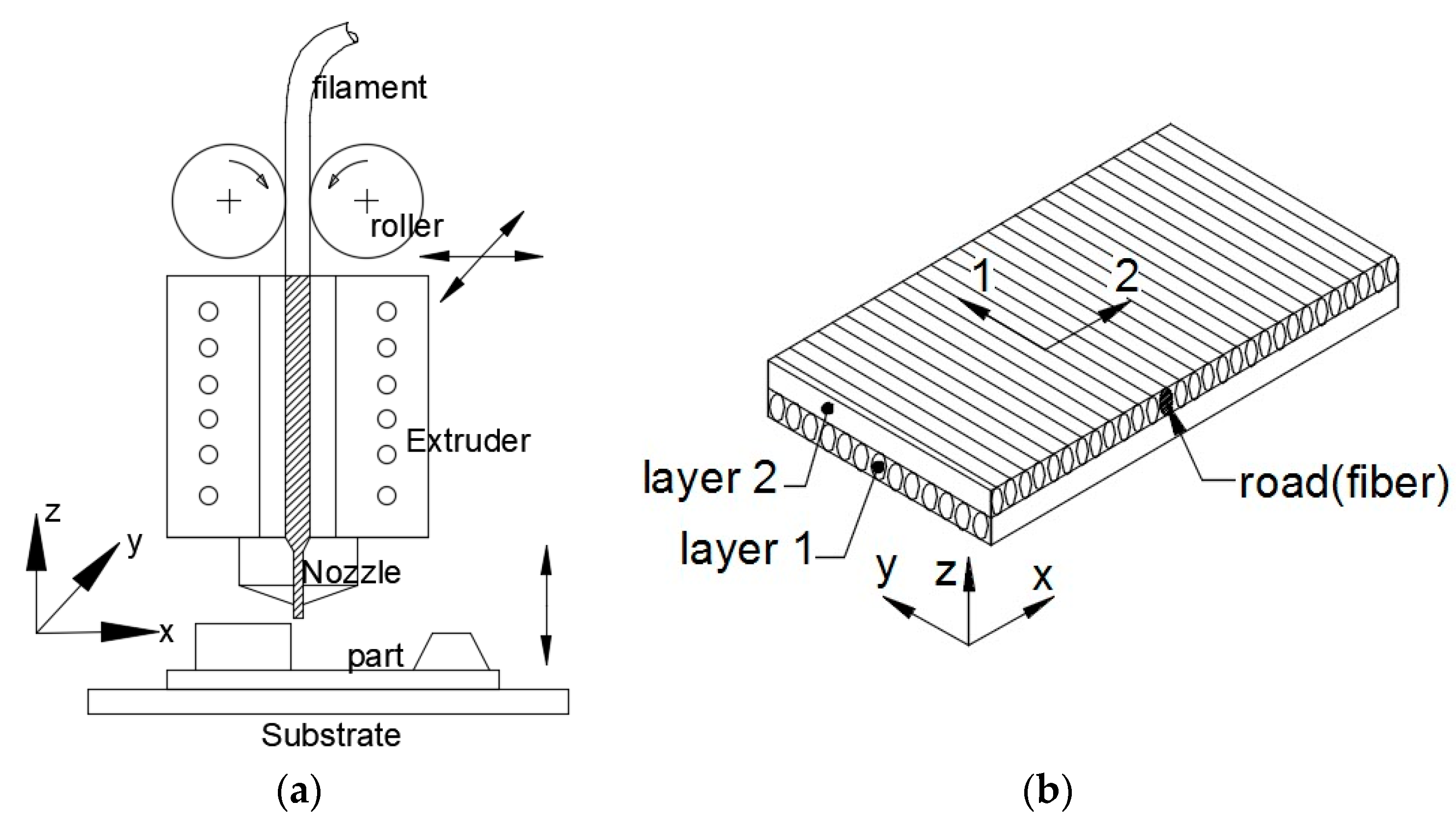
In FDM, the filament is melted in the extruder and the molten liquid is pushed through the nozzle to deposit on the substrate in the x-y plane. Then the molten material on the substrate cools and solidifies into what is referred as ‘road’. The schematic diagram of the FDM is shown in Figure 3a. Depositing the number of roads side by side forms a single layer. The several layers together act as laminate, such fabricated parts are considered as unidirectional fiber reinforced laminates. A two-layer plate fabricated with FDM process with an orientation of the roads in layer 1 and 2 at 0° and 90° to x-axis of the plate, respectively is shown in Figure 3b.
The process parameters of the FDM influence the mechanical properties of the part. The raster orientation while depositing molten material in each layer could be defined by the user. Different orientations of road in layers lead to anisotropy in the properties of the parts. Process parameters such as the gap between two adjacent roads and the percentage of infill while printing governs the strength of the part. The internal architecture of a part fabricated using FDM is not significantly different from that of fiber reinforced laminate structure. Therefore, the laminate theory for analysis of composite laminate can also be used for analysis of the FDM parts. The FDM processed parts resemble like laminate structures and therefore these parts can be characterized with classical laminate theory. The constitutive relation for a lamina is available in Equation (8) and is rewritten here
The global coordinate system (x, y, z) for a laminate plate and local coordinate system (1, 2, 3) for a lamina are considered. Strains of the laminate from classical laminate theory is written as
where and are mid-plane strains in the laminate; is the mid-plane shear strain in the laminate; and are bending curvature in the laminate; is the twisting curvature in the laminate and z is the distance from the mid plane in the thickness direction.
The constitutive relation for a lamina is written as
where are transformed material constants, the elements of are given as
where is a transformation matrix, T is given as
where c is , s is and is the fiber orientation in anticlockwise direction to the x-axis.
The resultant force and moment per unit width for a laminate with N number of layers are expressed as
Using Equations (18) and (19) and Equations (22) and (23) become
where Nxx and Nyy represent the normal forces per unit width in the x and y directions, respectively; Nxy is shear force; Mxx and Myy denote the bending moments in the yz and xz planes; Mxy is the twisting moment and [A], [B] and [D] are the extensional stiffness matrix, coupling stiffness matrix and bending stiffness matrix for the laminate, respectively. The matrices [A], [B], [D] are functions of each lamina stiffness matrix [Q] and the distance from mid plane of the laminate to the laminas and the stiffness matrices written as
The mid-plane strains and curvatures can be calculated from Equations (25) and (27), once we know the normal force and moment acting on a lamina. A symmetric laminate layup will have identical lamina material, thickness and fiber orientation located at an equal distance above and below the mid-plane of the laminate. For a symmetric laminate, the coupling matrix [B] = [0] and therefore there is no extension-bending coupling. Then, the strains for a symmetric laminate subjected to in-plane forces are given from Equation (25) as
In the uniaxial tensile test, the load is applied in the x direction and for laminate thickness h, then the in-plane forces for this load case become , Nyy = 0 and Nxy = 0. The stress-strain relation for uniaxial tensile test is , using these above relations the modulus of elasticity along the x direction is calculated as follows
For instance, if the Exx of the laminate is calculated from Equation (30), it is required to have the lamina’s elastic moduli such as E1, E2, G12, ν12. These constants are found from the FE simulation of tensile testing mentioned Section 2.2. Using these constants, the matrix [A] can be obtained and Exx of the laminate calculated using Equation (30).
To validate the calculated Exx of the laminate, experimental work is carried out to find Exx from the stress-strain curve of the tensile test. Once it is clear that the Exx obtained from experimental and numerical results is in agreement, then it can be said that the printed 3D parts via FDM can be characterized using laminate plate theory. In the analysis of the FDM processed parts, the classical laminate plate theory could be employed to characterize their mechanical behavior.
3. FE Methodology
In this section, finite element modeling of mesostructure of the FDM processed part is described. The FE modeling of mesostructure of an FDM processed layer and its behavior as a lamina material is demonstrated. Based on this, the finite element procedure is adopted to find the elastic moduli for a particular mesostructure of the FDM processed part. In the present work, the ABS polymer filament material properties available in [3] are employed in the FE analysis.
In the finite element model of an FDM processed part, the mesostructure of the part is considered. The mesostructure of the part basically will have roads and these are formed when deposited molten material is solidified on the bed. The roads are deposited side by side to form a layer and two adjacent roads in a layer share a common edge and the roads in the adjacent layer share a common surface. Mechanical properties of the part depend on the bonding strength between the roads in a layer and also in adjacent layers. The bonding strength is governed by the polymerization that takes place across interface of the adjacent roads during solidification [9]. Furthermore, the material extruded from the FDM machine nozzle has a circular cross section but when the material being deposited upon the bed then its cross section would become elliptical [9]. The FDM processed part will have pores, which are inherent to the process. Also, the size and shape of the pores influence the mechanical properties of the part [6]. The effect of size and shape of the voids on the mechanical properties is also investigated for different architecture of mesostructures in the present work. The connection of finite elements between the roads and layers as per bond formation during fabrication of the parts. The elliptical cross section roads are modeled with 3D linear finite elements, hexahedron and the connection between two adjacent roads have common surface of the finite elements, as shown in the Figure 4a. The cross section of a road is modeled with six finite elements as shown in Figure 4a, so that the mesh is fine enough to get accurate results. It is assumed that in the finite element modeling the roads of FDM processed parts have uniform cross section and are evenly spaced with negative air gap (10% overlap) between them in a layer. Also, perfect bond exists between the adjacent roads as well as between layers. In the present analysis, the elliptical size of the road for first two mesostructures is 0.50 mm major axis length (2y) and 0.317 mm minor axis length (2z) as shown in Figure 4a. The mesostructure images of FDM printed parts are taken using an optical microscope, BX41M-LED from Olympus Corporation, Center Valley, PA, USA and a digital camera from Metlab Corporation, St Catharines, ON, Canada. All micro images shown in this paper are captured with 5X magnification.
3.1. FE Modeling of a Layer and Its Behavior as a Lamina
The FE modeling of an FDM processed layer and its treatment as a lamina material is presented. Here, two different finite element models of simple single layer rectangular plate with different material properties are considered but of same length (L = 100 mm), width (W = 20 mm) and volume. Let us consider first model (model 1), where the layer that is obtained by FDM process (Figure 4a, layer1) behave as a lamina and is replicated in finite element model with 3D linear finite elements. This means that the mesostructure of the layer is modeled with 3D continuum finite elements. The mesostructure replication in FE modeling can capture the actual mechanical behavior of the FDM fabricated parts. In the second model (model 2), where the lamina as a bulk material is considered. The lamina treated as a two dimensional plate and modeled with 2D linear finite elements. As discussed earlier that the layer of FDM processed parts behaves as a lamina, which is an orthotropic material. The second model is actually a layer of FDM processed part but treated as a bulk lamina material. The elastic moduli of the materials for model 1 is isotropic and model 2 is orthotropic, are taken from Li et al. [3] and the elastic moduli are presented in Table 1. The virgin material that is used in fabricating parts using FDM is isotropic but the layers in the final printed part act as lamina material. The final material properties of the printed part differ from that the virgin material and therefore, the model 1 is treated with isotropic material and model 2 is treated as lamina material.
The important feature in this study is that the model 1 accounts the isotropic constitutive relation (Equation (1)) and the model 2 accounts the orthotropic constitutive relation (Equation (8)). The main differences between the models 1 and 2 are finite element modeling and the constitutive relation of the material. They are subjected to same magnitude of uniaxial tensile load, then the elasto-static analysis is carried out. The total strain energy of the deformed member calculated using Equation (5) and can be obtained from finite element simulation. The strain energy obtained for the model 1 is 198.93 N-mm and for the model 2 is 208.19 N-mm. The strain energy difference between the models is 1.44 % and it could be due to inexact replication of the actual geometry that was used in experiments [3] to find elastic moduli, which are considered in this analysis. The strain energies for both cases in well agreement, therefore the strain energy obtained for the model 1 can be equated to the strain energy of the model 2.
Further, from this study it is evident that the mesostructure replication in the finite element model for an FDM processed layer behave as a lamina. It is obvious that this approach can be used in the finite element model of the tensile specimens to find the elastic moduli of a layer of FDM processed tensile specimens instead of conducting experiments. Moreover, the experimental approach is time consuming and expensive, so the numerical approach is adopted here and the present numerical results have been validated with existing experimental results in literature. The elastic moduli of the layers are found numerically by simulating three different tensile test cases, in each case the orientation of road in a layer would be at an angle to the axis of the loading. The mesostructure of tensile test specimens that would be obtained from FDM process is replicated in the finite element models and uniaxial tensile tests are simulated to calculate the strain energies of the specimens. Then the strain energies obtained from the simulations of three cases are used in the Equations (11), (13) and (15) to calculate the elastic moduli of the lamina as explained in Section 2.
3.2. FE Analysis to Find Elastic Moduli of a Layer
This section describes the procedure for calculation of the elastic moduli for a particular mesostructure of the printed part. For this, three different tensile specimens as per standards mentioned earlier are modeled in a commercially available finite element software. Initially, the regular mesostructure of an FDM processed tensile specimens are replicated in the finite element model. The specimens are modeled with 3D finite elements as explained in the previous section. The size of the road is equal to the layer thickness. The FE model of the tensile specimen has eight layers and all layers have equal thickness. The time for simulations is around 15 min and simulations are carried out using an HP Z840 workstation with only one Intel Xeon processor. Most commonly used filament materials in a fused deposition process are thermoplastics. The ABS-P400 filament material properties available in the literature [3,5] are considered for the validation of the present finite element procedure. The isotropic material properties of the filament are E = 2230 MPa, ν = 0.34, given in Table 1. For the calculation of E1, the case 1 is to be simulated as explained in Section 2, the roads in this case are oriented at 0° to the axis of the loading. The specimen is subjected to unit displacement as a tensile load at one end of the specimen along the x-axis and the other end is fixed, then the FE analysis is carried out. The total strain energy (U) obtained from this simulation is 262.20 N-mm and the displacement () is 1 mm. Upon substituting the strain energy and displacement in Equation (11), the unknown elastic constant E1 is calculated, which is 1851.9 MPa. The longitudinal strain is 0.0087, lateral strain is −0.0030 and then the Poisson’s ratio is 0.34.
For the calculation of E2, the case 2 analysis should be carried out and in this case that the roads are oriented at 90° to the axis of the loading in the specimen. The finite element model for this case is developed. In this case also, unit displacement is applied as a tensile load along x-axis at one end of the specimen and other end is fixed and then analysis is carried out. The total strain energy obtained from simulation of this case is 544.16 N-mm and applied displacement is 1 mm. Using these values in Equation (13), the unknown elastic constant E2 is calculated and the value is 1501.3 MPa.
For the calculation of G12, the FE analysis should be carried for the case 3 as explained in Section 2. In this case, the roads are oriented at 45° anticlockwise direction to the axis of the loading in the tensile specimen. The mesostructure of the layer that would be obtained from FDM process is replicated in the finite element model of tensile specimen. Then specimen subjected to uniaxial tensile load and boundary conditions; unit displacement almond x-axis as a load at one end of the member and other end is fixed. Here the roads are oriented at off-axis of the loading, therefore the roads subject to shear deformation and this is how shear modulus is calculated. The total strain energy obtained from simulation of this case is 232.14 N-mm and the displacement along x-axis is 1 mm. Using these values in Equation (15), the modulus of the elasticity along x-axis, Ex is calculated and its value is 1640.8 MPa. The unknown elastic constant shear modulus G12 is obtained from Equation (16) using elastic constants found earlier and the G12 value is 625.4 MPa. The elastic moduli of an FDM processed layer, which behave as lamina, obtained from three finite element simulations are given in Table 2. The present numerical results are evaluated with existing experimental results in the literature.
In the following section, the above methodology is employed to investigate the effect of the arrangement of fibers in a mesostructure, the thickness of the fiber, the shape of the fiber and the bonding between the fibers on the elastic moduli of a material of the printed parts. Also, influence of fiber orientation in the laminates, which is lamina layup, on the stiffness of the laminate is studied using experimental work and laminate theory.
4. Results and Discussion
Initially, an evaluation of the present numerical results with available experimental results is discussed. Then the influence of a different architecture of mesostructure that would be obtained from FDM process is considered for investigation of its influence on mechanical properties of the parts. Also, the effect of the layer thickness, road shape and air gap on the elastic moduli is investigated. Then, the elastic moduli are employed to characterize the mechanical behavior of the FDM processed parts using classical laminate theory in Section 4.1 and the results are validated with experimental results. Finally, the Section 4.2 discusses an application of the present work for FDM printed parts.
The difference in the experimental results in Table 2 by researchers is a result of process parameters such as air gap, percentage of infill, substrate temperature maintained while building tensile specimens for experiments. Also, the difference in the present numerical results and experimental results could be the same reason. Further, in the present finite element models it is presumed that there exists perfect bonding between the adjacent roads as well as between the layers but this is not the case in the actual printed parts. Li et al. [3] and Rodriguez et al. [5] adopted ASTM D3039 tensile testing procedure for finding elastic properties of the lamina. Casavola et al. [27] adopted the ASTM D638 and ASTM D3518-94 tensile testing procedures for finding the in-plane Young’s modulus and shear modulus, respectively. The shear modulus obtained using Equation (16) for the case of Casavola et al. [27] is 542.96 MPa. As there were not well defined testing standards exist for 3D printed parts, researcher conducted tests as per ASTM D638 and ASTM D3039. In present analysis, all FE models are developed as per ASTM D3039 standards to investigate the influence of the type of mesostructure architecture, layer thickness, road shape and air gap on the properties of the part.
Next, a different architecture of mesostructure (tightly packed) of the FDM printed part is considered for investigation of its influence on the mechanical properties of a material. The FE model of tightly packed mesostructure and the microscopic image of printed sample are shown in Figure 5a,b, respectively. In the previous case, the roads are aligned in the same pattern in each layer as shown in Figure 4b. In this case, the roads in the consecutive layer are offset by a certain distance such that the road falls between the gap of the roads of the previous layer as shown in Figure 5b. The previous configuration has diamond shape voids between the adjacent roads and the later configuration has triangle shape voids. The road (hatched area) in a layer is surrounded by four adjacent roads in the previous case (Figure 4a) whereas in this case, the road is surrounded by six adjacent roads, as shown in Figure 5a. The roads are tightly packed and also the percentage of the material per unit volume is higher in the later mesostructure. The void density in the mesostructure of first case is higher since roads are not tightly packed. The common printing practice gives mesostructure of the first case, shown in Figure 4b but with certain changes in the geometry of the part as well as adjusting the process parameters would give the mesostructure of the present case.
Let us consider tensile specimens with tightly packed mesostructure. Three specimens are replicated in the finite element model to calculate elastic moduli of a layer. Then the same procedure as explained above for three cases is repeated to find the elastic moduli. The elastic moduli for this mesostructure are given in Table 3. The shear modulus and Young’s modulus in transverse direction are higher for this type of mesostructure compare to the regular mesostructure. This is due to the tightly packed mesostructure and each road is surrounded by six adjacent roads, whereas in the earlier case each road is surrounded by four adjacent roads. Also, the percentage of material in a unit volume is higher in tightly packed mesostructure compare to that of regular mesostructure. Therefore, the tightly packed mesostructure provides higher stiffness and this is the reason the elastic moduli are higher. The Young’s modulus in transverse direction is found from case 2 simulation, in which the fiber is oriented along y-axis. This elastic modulus (E2) for this architecture of mesostructure is higher compare to that of regular mesostructure. This is because of more material present across the section of the specimen. Further, when the force P is applied along x-axis in tensile test, the weakest cross section in the part would be cross section A-A and B-B for the regular mesostructure and tightly packed mesostructure, respectively as shown in Figure 6a,b. Also, the void density (dark areas) along the weakest cross section in the tightly mesostructure is lower compare to that of regular mesostructure. Therefore, the present type of mesostructure will have higher strength.
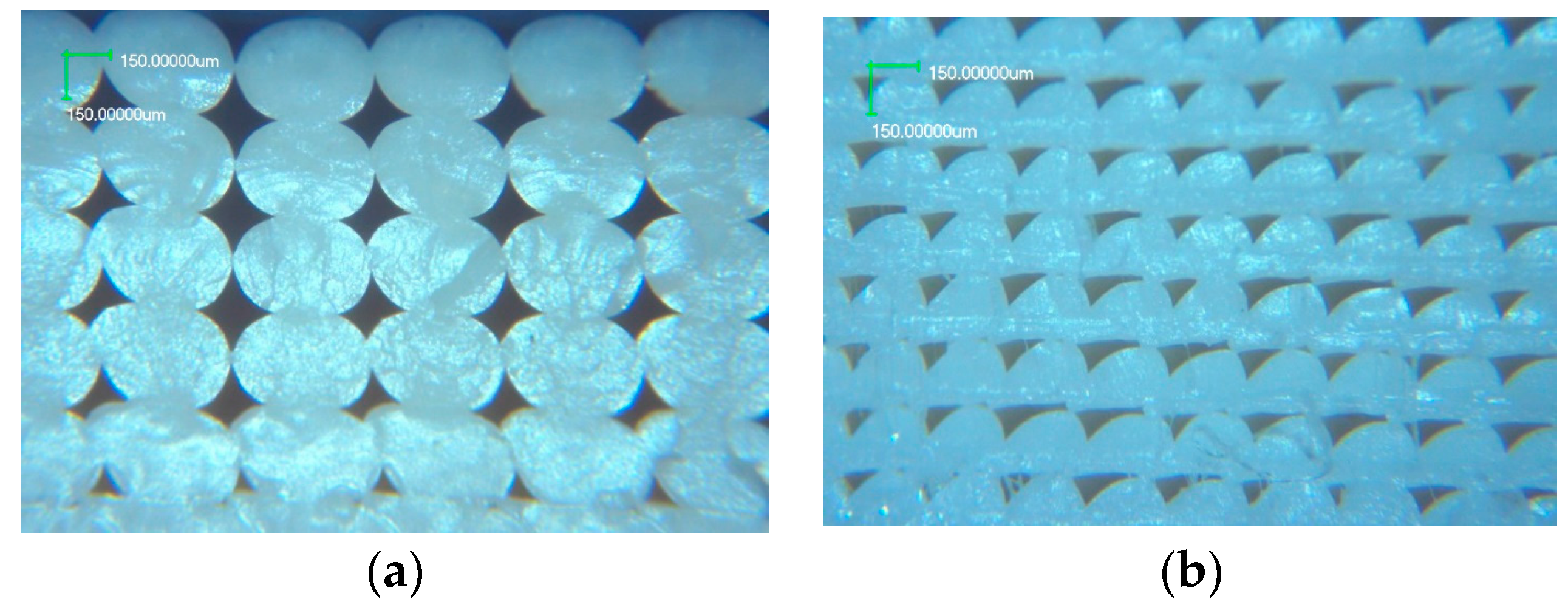
Next, the layer thickness and shape of the road influence on elastic properties is investigated. Here, the tensile specimen with 14 layers has lower layer thickness than that of specimen with 8 layers. The cross section size of the road for thin layer model is 2y = 0.26 mm, 2z = 0.18 mm. As described earlier, the finite element simulations are carried out to find the elastic moduli of a layer. The elastic moduli obtained from tensile specimens with thin layers and thick layers are presented in Table 4. It is seen that the no significant difference exists in the elastic properties of the thin and thick parts. The size of the voids differ and the number of voids are more in the thin layer specimen but the void density per unit area in both cases nearly same. In the case of the thin layer, the void size is small compare to the thick layer case. The mesostructure of the printed samples with higher layer thickness and lower layer thickness are shown in Figure 7a,b, respectively.
The effect of the shape of the road on the elastic moduli of a layer is now considered. The shape of the road that would be obtained is elliptical during solidification. The other process parameters such as flow rate and printing speed would also change the cross-section shape of the road. Let us say that we have an extruder in the FDM machine, which can provide a larger road shape such that the major axis of the ellipse is 0.64 mm, as shown in Figure 8a. Then this kind of mesostructure is replicated in the FE tensile specimen models to carry out simulations to find the elastic moduli and the results are presented in Table 4. The increase in the cross-sectional area of the road does not have much effect on the elastic properties, however there is significant improvement in the Young’s modulus in the transverse direction (E2).
Next, the effect of the other process parameter—air gap—on the mesostructure and its elastic properties is investigated. A regular printing process prints the parts with a 10% overlap between the roads—all previous cases are based on this and then the contact between the roads in a layer is not wider. In the present case, the overlap of 20% of the road size between the adjacent roads is considered. When an air gap less than zero is considered in the printing, it means the adjacent roads are overlapped and the bonding strength between the roads in a layer would be high. Moreover, the void size in this case means the mesostructure would be smaller compared to the regular mesostructure by adding more material to the part. Also, the contact area between the adjacent roads would be higher and the mesostructure for this case is shown in Figure 8b. Therefore, the elastic moduli for the 20% overlapping mesostructure are better than those for the regular mesostructure and are given in Table 5.
4.1. Characterization of FDM Parts Using CLT
The FDM process is a layer upon layer deposition of material and parts fabricated with such parts resemble as laminate structures. The mechanical behavior of laminate structures is characterized with classical laminate theory in the analysis. The laminate theory would be employed in the analysis of the FDM parts. The Matlab program was developed based on the classical laminate theory to characterize the mechanical behavior of the FDM processed parts.
The Ultimaker FDM machine equipped with nozzle diameter is 0.40 mm is used in building tensile specimens. Commercially available ABS-P400 filament material is used for printing tensile specimens. The process parameters employed for printing are; extruder temperature 230 °C, substrate temperature 80 °C, printing speed 60 mm/s, number of shells 1, air gap is −10%(overlap), layer height 0.317 mm and infill density 100 percent. All layers in the tensile specimen have equal thickness. The elastic moduli of a layer obtained from the above numerical simulations would be used in the laminate theory to find the Young’s modulus (Exx) of the specimen along x-axis. This value would be validated with experiments results obtained from tensile testing. Here, symmetric laminates are considered and the uniaxial tensile load is applied along x-axis to the laminates, the Young’s modulus along the axis of the load is calculated from the program using Equation (30). The Matlab program has the following sequence of steps:
- Elastic moduli (E1, E2, G12, ν12) of a layer for the regular mesostructure obtained from Section 3.2 FE simulations are taken as lamina elastic properties.
- Stiffness matrix for a laminate is calculated using Equation (20).
- Stiffness matrices A, B, D for a laminate are calculated using Equation (28).
- For a symmetric laminate, equate the matrix B = 0 and for uniaxial tensile load case D = 0.
- Consider the only existing term from resultants Equations (25) and (27),
- Apply uniaxial tensile load, Nxx, then calculate Exx of the laminate using Equation (30) as explained in Section 2.3
Here, four different symmetric lamina layup are considered for investigation as given in Table 6. The tensile specimens as per ASTM D3039 standards are built for four different layup cases. The specimen dimensions; gage length 130 mm, width 25.4 mm and thickness is 2.54 mm. For each laminate layup case, 6 tensile specimens are built. A total of 24 tensile specimens are printed for four different laminate layup. Then uniaxial tensile tests are conducted to find Exx value from stress-strain curve. The MTS tensile machine with a load cell capacity of 10 kN is used for the tensile testing of FDM processed specimens. Uniaxial tensile testing of the printed laminate is shown in the Figure 9. The load versus displacement data is recorded during tensile testing and then the stresses and strains are calculated for corresponding recorded data. Laser extensometer is used for recording the displacement while testing. The line slope in linear stress-strain data of the experiments gives the Young’s modulus Exx for each laminate. Then mean Young’s modulus and standard deviation (SD) is calculated for sample size of six Exx for a particular laminate layup case. The obtained results from the laminate theory are presented in Table 7 and results are validated with experimental results. Further, the standard deviation of the experimental results is also provided. The experimental results depend on the quality of the printing [9] such as bonding formation between the fibers and as well as between the layers. The strength of the bond also depends on the process parameters such as extruder temperature, printing speed, cooling rate and chamber environment. Moreover, the printed specimens are not in exact size as represented in numerical models because of the low printer resolution. Therefore, the difference between experimental and laminate theory results is expected. It is seen from the Table 7 that the laminate theory results are comparable with that of experimental results and therefore the laminate theory could be used to characterize the mechanical behavior of the fused deposition processed parts.
4.2. Application
The present FEA procedure has two main applications; firstly, estimating the final mechanical properties of a material of the FDM processed part with different mesostructures. The estimated final mechanical properties of the material for a particular mesostructure will be considered in the constitutive relation of a material for characterization of the mechanical behavior of the parts. Secondly, mechanical behavior characterization of the parts can be done using laminate theory. The build orientation of a part and raster direction govern the type of mesostructure obtained while printing a 3D part having different shapes of cross sections. The parts with different mesostructure will have different material properties and therefore the mechanical behavior of the mesostructures will vary. Also, the mesostructures perform differently under different load conditions. For example, the 3D printed part having tightly packed mesostructure provides higher stiffness along and across the fiber direction when compare to that of regular mesostructure. Also, the parts having negative air gap mesostructure have better mechanical properties when compare to parts having zero air gap mesostructure.
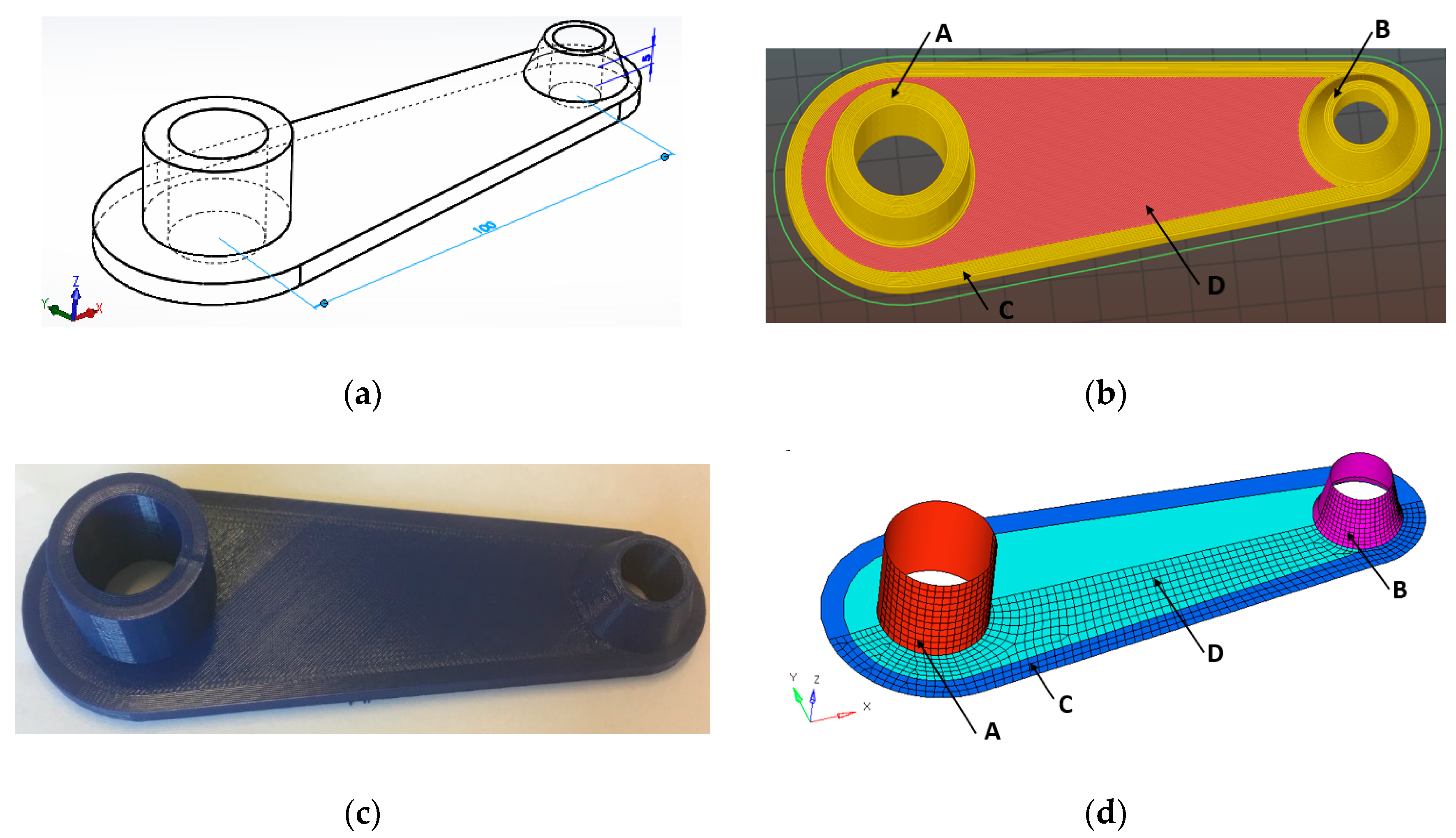
Let us consider a connecting component which is to be fabricated via FDM, which has a base plate on the x-y plane and cylindrical cross sections as shown in Figure 10a. The cylindrical section on left end of the component is concentric and other is a tapered cylindrical section and these are an integral part of the base plate of the component. The CAD model of the connecting part is shown in Figure 10a. The STL file of the component is imported into the slicer software of the FDM machine. The slicer generates G-code based on user defined printer settings for layer upon layer deposition of a material as shown in Figure 10b. In the present case, the build orientation of the part is that its base plate is located on x-y plane of substrate of the printer. The model has four different regions as indicated in Figure 10b. The mesostructure in each region is different and the mesostructure of the corresponding region that would appear in the final printed component is presented in Table 8. As discussed in previous sections, the mechanical behavior depends on the mesostructure. The correct elastic moduli should be accounted in the FEA of the component for mechanical behavior characterization under different mechanical loads. The elastic moduli calculated for different mesostructures from previous sections would be useful in the characterization of mechanical behavior of the component. The elastic moduli calculated for the respective mesostructure in the previous section will be used in the stiffness matrix of a material for FEA. Furthermore, the component is treated as a laminated composite structure. Therefore, the finite elements based on classical laminate theory would be adopted for the analysis. The mid surface of the component is extracted for the FEA and then the mid surface is modeled with laminated composite finite elements as shown in Figure 10d. Finally, the finite elements in different regions of the component are assigned with their respective elastic moduli (as presented in Table 8) for the FEA analysis of the component. Also, the type of laminates which exist in the component are presented in the Table 8.
The present FEA procedure assists the designer in understanding the mechanical performance of the FDM processed parts embedded with different mesostructures subjected to different load conditions. A better understanding of the mechanical performance of the parts under different load cases is important for reliable design. Furthermore, the designer can also tailor the mesostructure to get desired mechanical properties in a part to be fabricated via FDM. The mechanical behavior of the FDM processed parts subjected to different loads can be characterized using classical laminate theory as explained in this paper. In conclusion, the present simulation procedure is useful for characterization of mechanical behavior of a complex geometry part, which has different mesostructures fabricated via the FDM process.
5. Conclusions
In this paper, initially that the finite element procedure for finding the elastic moduli of the fused deposition processed parts is presented. It is seen that the strain energy obtained from the finite element model of the fused deposition processed layer and the lamina model is equal. So it is evident that the strain energy principle could be used to find the elastic moduli of a fused deposition processed layer numerically. The procedure for finite element modeling of mesostructures of the tensile specimens is described. Then the elastic moduli of a layer calculated from finite element simulation of tensile tests and results are found to be in agreement with existing experimental results in the literature. Then the influence of different architecture of mesostructures and the effect of size and shape of the voids on the mechanical properties are investigated. It is found that the tightly packed mesostructure possess better elastic moduli values than the regular mesostructure of the parts. It means that the tightly packed mesostructure of the part will have higher transverse and also shear elastic modulus but the Young’s modulus in the longitudinal direction is same in both cases. Also, the influence of the layer thickness, road shape and air gap on the elastic moduli is investigated. The elastic moduli obtained for the tightly mesostructure and the negative air gap mesostructure are similar. Further, they are approaching elastic properties of the virgin isotropic material. Then the classical laminate theory is adopted to characterize the mechanical behavior of the fused deposition processed parts. For this, tensile specimens are fabricated and experiments are conducted to validate the laminate theory results. It is observed that the results from the classical laminate theory and experiments are in well agreement. So, it is concluded that the classical laminate theory could be used to characterize the mechanical behavior in the analysis of the fused deposition processed parts. This study provides the finite element modeling of FDM processed parts to find the stiffness matrix and also it establishes the relationship between the mesostructure and the elastic moduli of the material of the FDM processed part.
Author Contributions
Madhukar Somireddy conceived and designed the experiments, also performed the analysis. Aleksander Czekanski supervised and provided the materials for the project.
Conflicts of Interest
The authors declare no conflict of interest.
References
- Kotlinski, J. Mechanical properties of commercial rapid prototyping materials. Rapid Prototyp. J. 2014, 20, 499–510. [Google Scholar] [CrossRef]
- Ahn, S.H.; Montero, M.; Odell, D.; Roundy, S.; Wright, P.K. Anisotropic material properties of fused deposition modeling ABS. Rapid Prototyp. J. 2002, 8, 248–257. [Google Scholar] [CrossRef]
- Li, L.; Sun, Q.; Bellehumeur, C.; Gu, P. Composite modeling and analysis for fabrication of FDM prototypes with locally controlled properties. J. Manuf. Process. 2002, 4, 129–141. [Google Scholar] [CrossRef]
- Bellini, A.; Güçeri, S. Mechanical characterization of parts fabricated using fused deposition modeling. Rapid Prototyp. J. 2003, 9, 252–264. [Google Scholar] [CrossRef]
- Rodríguez, J.F.; Thomas, J.P.; Renaud, J.E. Mechanical behavior of acrylonitrile butadiene styrene (ABS) fused deposition materials. Experimental investigation. Rapid Prototyp. J. 2001, 7, 148–158. [Google Scholar] [CrossRef]
- Agarwala, M.K.; Jamalabad, V.R.; Langrana, N.A.; Safari, A.; Whalen, P.J.; Danforth, S.C. Structural quality of parts processed by fused deposition. Rapid Prototyp. J. 1996, 2, 4–19. [Google Scholar] [CrossRef]
- Kulkarni, P.; Dutta, D. Deposition strategies and resulting part stiffnesses in fused deposition modelling. J. Manuf. Sci. Eng. 1999, 121, 93–103. [Google Scholar] [CrossRef]
- Kulkarni, P.; Marsan, A.; Dutta, D. A review of process planning techniques in layered manufacturing. Rapid Prototyp. J. 2000, 6, 18–35. [Google Scholar] [CrossRef]
- Sun, Q.; Rizvi, G.M.; Bellehumeur, C.T.; Gu, P. Effect of processing conditions on the bonding quality of FDM polymer filaments. Rapid Prototyp. J. 2008, 14, 72–80. [Google Scholar] [CrossRef]
- Durgun, I.; Ertan, R. Experimental investigation of FDM process for improvement of mechanical properties and production cost. Rapid Prototyp. J. 2014, 20, 228–235. [Google Scholar] [CrossRef]
- Ziemian, S.; Okwara, M.; Ziemian, C.W. Tensile and fatigue behavior of layered acrylonitrile butadiene styrene. Rapid Prototyp. J. 2015, 21, 270–278. [Google Scholar] [CrossRef]
- Rodriguez, J.F.; Thomas, J.P.; Renaud, J.E. Characterization of the mesostructure of fused-deposition acrylonitrile-butadiene-styrene materials. Rapid Prototyp. J. 2000, 6, 175–186. [Google Scholar] [CrossRef]
- Huang, B.; Singamneni, S. Raster angle mechanics in fused deposition modelling. J. Compos. Mater. 2015, 49, 363–383. [Google Scholar] [CrossRef]
- Tymrak, B.M.; Kreiger, M.; Pearce, J.M. Mechanical properties of components fabricated with open-source 3-D printers under realistic environmental conditions. Mater. Des. 2014, 58, 242–246. [Google Scholar] [CrossRef]
- Ning, F.; Cong, W.; Hu, Y.; Wang, H. Additive manufacturing of carbon fiber reinforced plastic composites using fused deposition modeling: Effects of process parameters on tensile properties. J. Compos. Mater. 2017, 51, 451–462. [Google Scholar] [CrossRef]
- Rezayat, H.; Zhou, W.; Siriruk, A.; Penumadu, D.; Babu, S.S. Structure-mechanical property relationship in fused deposition modelling. Mater. Sci. Technol. 2015, 31, 895–903. [Google Scholar] [CrossRef]
- Domingo-Espin, M.; Puigoriol-Forcada, J.M.; Garcia-Granada, A.A.; Llumà, J.; Borros, S.; Reyes, G. Mechanical property characterization and simulation of fused deposition modeling Polycarbonate parts. Mater. Des. 2015, 83, 670–677. [Google Scholar] [CrossRef]
- Zou, R.; Xia, Y.; Liu, S.; Hu, P.; Hou, W.; Hu, Q.; Shan, C. Isotropic and anisotropic elasticity and yielding of 3D printed material. Compos. Part B Eng. 2016, 99, 506–513. [Google Scholar] [CrossRef]
- Attar, H.; Ehtemam-Haghighi, S.; Kent, D.; Wu, X.; Dargusch, M.S. Comparative study of commercially pure titanium produced by laser engineered net shaping, selective laser melting and casting processes. Mater. Sci. Eng. A 2017, 705, 385–393. [Google Scholar] [CrossRef]
- Rodríguez, J.F.; Thomas, J.P.; Renaud, J.E. Mechanical behavior of acrylonitrile butadiene styrene fused deposition materials modeling. Rapid Prototyp. J. 2003, 9, 219–230. [Google Scholar] [CrossRef]
- Liu, X.; Shapiro, V. Homogenization of material properties in additively manufactured structures. Comput. Aided Des. 2016, 78, 71–82. [Google Scholar] [CrossRef]
- Ziemian, C.W.; Ziemian, R.D.; Haile, K.V. Characterization of stiffness degradation caused by fatigue damage of additive manufactured parts. Mater. Des. 2016, 109, 209–218. [Google Scholar] [CrossRef]
- Prashanth, K.G.; Shahabi, H.S.; Attar, H.; Srivastava, V.C.; Ellendt, N.; Uhlenwinkel, V.; Eckert, J.; Scudino, S. Production of high strength Al85Nd8Ni5Co2 alloy by selective laser melting. Addit. Manuf. 2015, 6, 1–5. [Google Scholar] [CrossRef]
- Attar, H.; Ehtemam-Haghighi, S.; Kent, D.; Okulov, I.V.; Wendrock, H.; Bӧnisch, M.; Volegov, A.S.; Calin, M.; Eckert, J.; Dargusch, M.S. Nanoindentation and wear properties of Ti and Ti-TiB composite materials produced by selective laser melting. Mater. Sci. Eng. A 2017, 688, 20–26. [Google Scholar] [CrossRef]
- Alaimo, G.; Marconi, S.; Costato, L.; Auricchio, F. Influence of meso-structure and chemical composition on FDM 3D-printed parts. Compos. Part B Eng. 2017, 113, 371–380. [Google Scholar] [CrossRef]
- Ahn, S.H.; Baek, C.; Lee, S.; Ahn, I.S. Anisotropic tensile failure model of rapid prototyping parts-fused deposition modeling. Int. J. Mod. Phys. B 2003, 17, 1510–1516. [Google Scholar] [CrossRef]
- Casavola, C.; Cazzato, A.; Moramarco, V.; Pappalettere, C. Orthotropic mechanical properties of fused deposition modelling parts described by classical laminate theory. Mater. Des. 2016, 90, 453–458. [Google Scholar] [CrossRef]
- Jones, R.M. Mechanics of Composite Materials, 2nd ed.; Taylor & Francis: Philadelphia, PA, USA, 1999. [Google Scholar]
Figure 1.
Dimensions of tensile specimens (a) fiber orientation along x-axis; (b) fiber orientation along y-axis, (c) fiber orientation 45° to x-axis.
Figure 1.
Dimensions of tensile specimens (a) fiber orientation along x-axis; (b) fiber orientation along y-axis, (c) fiber orientation 45° to x-axis.
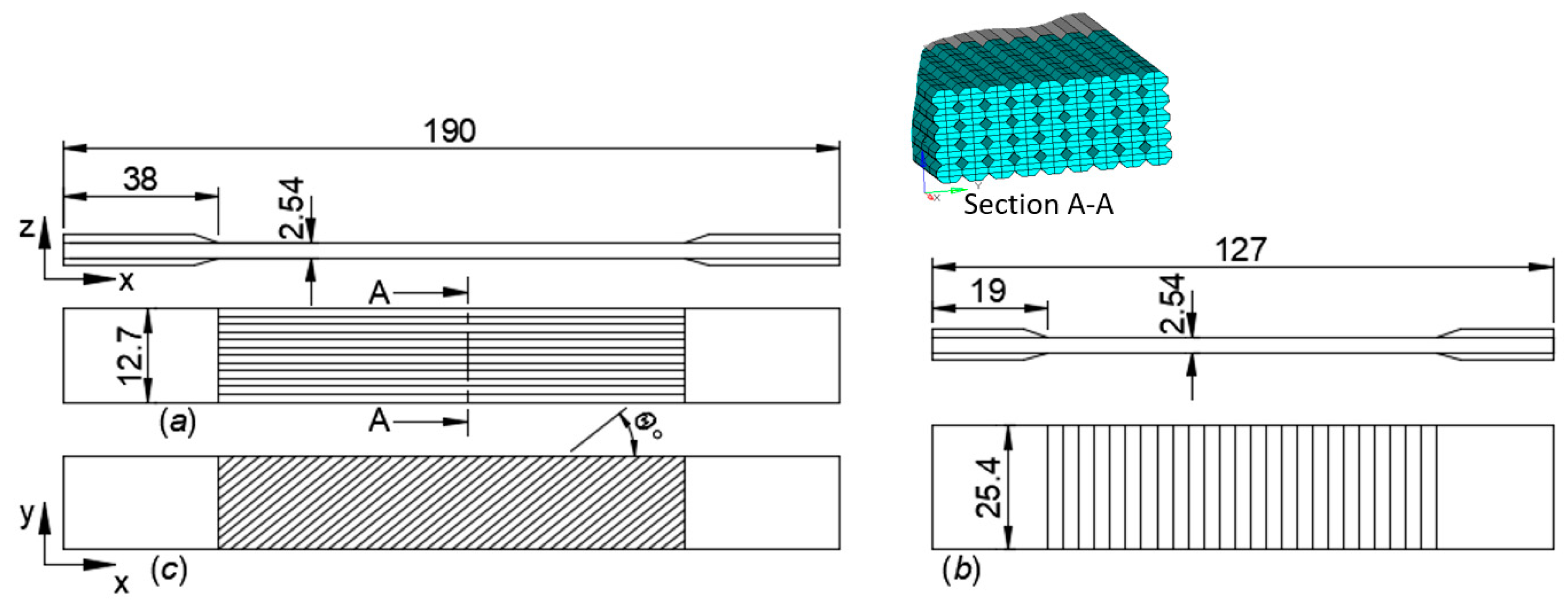
Figure 2.
Uniaxial tensile loading of laminate with fiber oriented (a) along axis of loading; (b) normal to axis of loading and (c) off axis to axis of loading.
Figure 2.
Uniaxial tensile loading of laminate with fiber oriented (a) along axis of loading; (b) normal to axis of loading and (c) off axis to axis of loading.

Figure 3.
(a) FDM process; (b) plate fabricated with FDM process in 0° and 90° raster orientation.

Figure 4.
Mesostructure of the FDM processed part (a) FE modeling of regular mesostructure (diamond voids); (b) microscopic image of the printed part.
Figure 4.
Mesostructure of the FDM processed part (a) FE modeling of regular mesostructure (diamond voids); (b) microscopic image of the printed part.
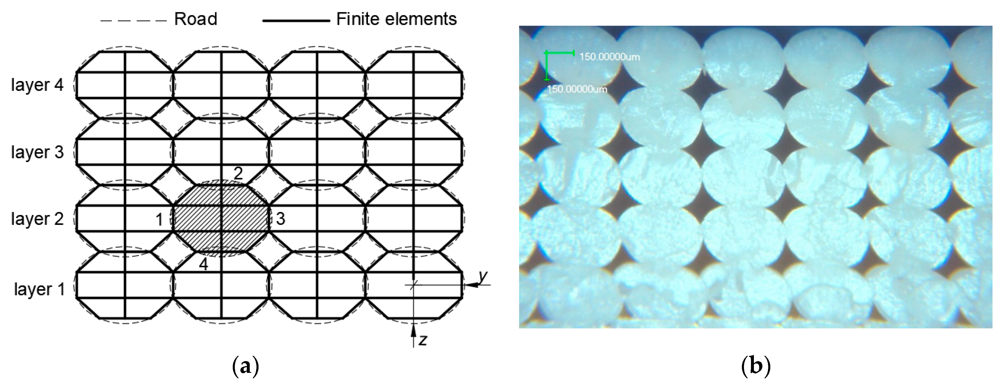
Figure 5.
Tightly packed mesostructure of the 3D printed parts via FDM (a) FE modeling; (b) microscopic image of the printed part.
Figure 5.
Tightly packed mesostructure of the 3D printed parts via FDM (a) FE modeling; (b) microscopic image of the printed part.
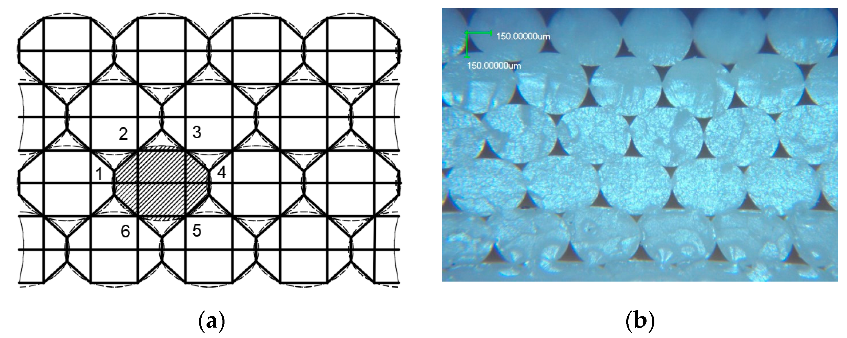
Figure 6.
Mesostructure of the tensile specimen subjected to uniaxial load (a) regular; (b) tightly packed mesostructure.
Figure 6.
Mesostructure of the tensile specimen subjected to uniaxial load (a) regular; (b) tightly packed mesostructure.

Figure 7.
Mesostructure of the printed part (a) higher layer thickness, 0.317 mm; (b) lower layer thickness, 0.181 mm.
Figure 7.
Mesostructure of the printed part (a) higher layer thickness, 0.317 mm; (b) lower layer thickness, 0.181 mm.

Figure 8.
Mesostructure of the FDM processed part (a) bigger cross section of the road; (b) regular road shape with 20% overlap.
Figure 8.
Mesostructure of the FDM processed part (a) bigger cross section of the road; (b) regular road shape with 20% overlap.
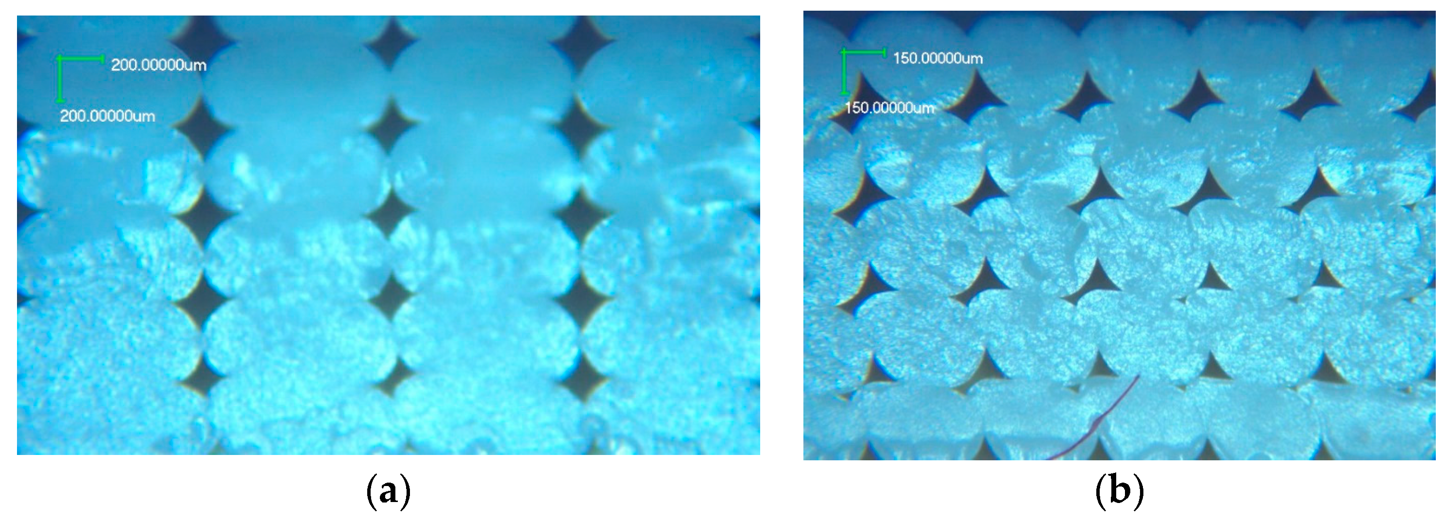
Figure 9.
Tensile testing of the printed specimen.
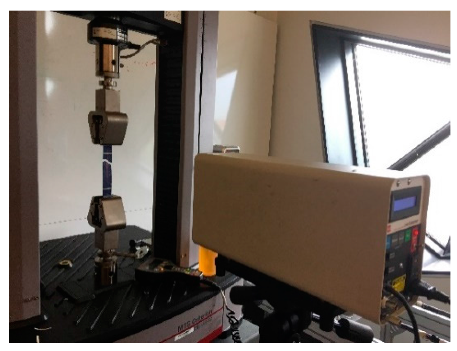
Figure 10.
FDM fabricated component and its FE model (a) CAD model (b) FDM Slicer model for printing; (c) FDM fabricated part (d) laminated composite 2D finite element model for FEA.
Figure 10.
FDM fabricated component and its FE model (a) CAD model (b) FDM Slicer model for printing; (c) FDM fabricated part (d) laminated composite 2D finite element model for FEA.


Table 1.
Material properties, [3].
Table 1.
Material properties, [3].
| Model 1 | E = 2230 MPa, ν = 0.34 |
| Model 2 | Ex = 2137.7 MPa, Ey = 1203.4 MPa, νxy = 0.34, Gxy = 416.6 MPa |
Table 2.
Layer properties of the part processed by FDM for regular mesostructure.
| Elastic Moduli | Experimental | Present Numerical | ||
|---|---|---|---|---|
| Li et al. [3] | Rodriguez et al. [5] | Casavola et al. [27] | ASTM D3039 | |
| , MPa | 2030.9 | 1972 | 1790 | 1851.9 |
| , MPa | 1251.6 | 1762 | 1150 | 1501.3 |
| 0.34 | 0.37 | 0.34 | 0.34 | |
| , MPa | 410.0 | 676 | 808.5 | 625.4 |
Table 3.
Layer properties of the part for regular and tightly packed mesostructure.
| Elastic Moduli | Regular Mesostructure | Tightly Packed Mesostructure | Difference, % |
|---|---|---|---|
| , MPa | 1851.9 | 1850.4 | −0.01 |
| , MPa | 1501.3 | 1806.1 | 16.8 |
| 0.34 | 0.35 | 2.85 | |
| , MPa | 625.4 | 670.4 | 6.71 |
Table 4.
Layer properties of the part processed by FDM for different mesostructures.
| Elastic Moduli | Regular Elliptical Shape 1 | Elliptical Shape 2 | |
|---|---|---|---|
| 8 Layers | 14 Layers | 8 Layers | |
| , MPa | 1851.9 | 1861.7 | 1852.8 |
| , MPa | 1501.3 | 1505.6 | 1632.7 |
| 0.34 | 0.342 | 0.36 | |
| , MPa | 625.4 | 626.0 | 635.8 |
Table 5.
Layer properties of the part processed by FDM for different air gap parameters.
| Elastic Moduli | Regular Mesostructure | 20% Overlap Mesostructure | Difference, % |
|---|---|---|---|
| , MPa | 1851.9 | 1940.9 | 4.5 |
| , MPa | 1501.3 | 1737.9 | 13.6 |
| 0.34 | 0.344 | 1.0 | |
| , MPa | 625.4 | 679.3 | 7.9 |
Table 6.
Elastic constants of a layer and symmetric lamina layup of the tensile specimen.
| Elastic Moduli of a Layer: E1 = 1851.9 MPa, E2 = 1501.3 MPa, ν12 = 0.34, G12 = 625.4 MPa | |
|---|---|
| Layup 1 | [0°, 30°, 0°, 30°]S |
| Layup 2 | [0°, 60°, 0°, 60°]S |
| Layup 3 | [0°, 90°, 0°, 90°]S |
| Layup 4 | [45°, −45°, 45°, −45°]S |
Table 7.
Modulus of elasticity of the laminate from classical laminate theory.
| Exx, MPa | Experimental ± SD | Present, CLT | Difference, % |
|---|---|---|---|
| Layup 1 | 1755.2 ± 28 | 1795.3 | 2.24 |
| Layup 2 | 1668.8 ± 27 | 1709.7 | 2.39 |
| Layup 3 | 1657.4 ± 43 | 1678.5 | 1.25 |
| Layup 4 | 1577.4 ± 77 | 1647.6 | 4.26 |
Table 8.
Mesostructures in a connecting component and their elastic moduli.
| Regions | Mesostructure (Ref Figure) | Elastic Moduli | Laminate and Its Thickness |
|---|---|---|---|
| Region A | Regular (Figure 4b) | Table 2 | Unidirectional, t = 5 mm |
| Region B | Tightly packed (Figure 5b) | Table 3 | Unidirectional, t = 2 to 6 mm |
| Region C | Elliptical shape2 (Figure 8a) | Table 4 | Unidirectional, t = 5 mm |
| Region D | Overlap (Figure 8b) | Table 5 | Bidirectional, t = 5 mm |
© 2017 by the authors. Licensee MDPI, Basel, Switzerland. This article is an open access article distributed under the terms and conditions of the Creative Commons Attribution (CC BY) license (http://creativecommons.org/licenses/by/4.0/).
Share and Cite
MDPI and ACS Style
Somireddy, M.; Czekanski, A. Mechanical Characterization of Additively Manufactured Parts by FE Modeling of Mesostructure. J. Manuf. Mater. Process. 2017, 1, 18. https://doi.org/10.3390/jmmp1020018
AMA Style
Somireddy M, Czekanski A. Mechanical Characterization of Additively Manufactured Parts by FE Modeling of Mesostructure. Journal of Manufacturing and Materials Processing. 2017; 1(2):18. https://doi.org/10.3390/jmmp1020018
Chicago/Turabian StyleSomireddy, Madhukar, and Aleksander Czekanski. 2017. "Mechanical Characterization of Additively Manufactured Parts by FE Modeling of Mesostructure" Journal of Manufacturing and Materials Processing 1, no. 2: 18. https://doi.org/10.3390/jmmp1020018