Evaluation of Altitude Sensors for a Crop Spraying Drone
by
 , and
, and
Matheus Hentschke
1,2, 
Edison Pignaton de Freitas
1,*,
Carlos Henrique Hennig
2 and
Igor Caike Girardi da Veiga
1 1
Federal University of Rio Grande do Sul (UFRGS), Porto Alegre, RS 90035-190, Brazil
2
Skydrones Avionics Technology, Porto Alegre, RS 91020-030, Brazil
*
Author to whom correspondence should be addressed.
Drones 2018, 2(3), 25; https://doi.org/10.3390/drones2030025
Submission received: 2 July 2018
/
Revised: 20 July 2018
/
Accepted: 26 July 2018
/
Published: 1 August 2018
Abstract
:This work aims to study and compare different range finders applied to altitude sensing on a rotating wings UAV. The specific application is the altitude maintenance for the fluid deployment valve aperture control in an unmanned pulverization aircraft used in precision agriculture. The influence of a variety of parameters are analyzed, including the tolerance for crop inconsistencies, density variations and intrinsic factors to the process, such as the pulverization fluid interference in the sensor’s readings, as well as their vulnerability to harsh conditions of the operation environment. Filtering and data extraction techniques were applied and analyzed in order to enhance the measurement reliability. As a result, a wide study was performed, enabling better decision making about choosing the most appropriate sensor for each situation under analysis. The performed data analysis was able to provide a reliable baseline to compare the sensors. With a baseline set, it was possible to counterweight the sensors errors and other factors such as the MSE for each environment to provide a summarized score of the sensors. The sensors which provided the best performance in the used metrics and tested environment were Lightware SF11-C and LeddarTech M16.
1. Introduction
In agriculture, the pulverization of fertilizers and pesticides is of prime importance. The manned aircraft spraying is one of the most used methods for this activity due to its high speed, being able to cover big areas in a short time. As a drawback, for smaller areas such as farm borders or uneven geometries, this method is not viable. For these scenarios, farmers usually resort to hand spraying [1]. As an alternative, a crop spraying drone can be of great help due to its speed and accuracy. As an additional advantage, the drone can be programmed to do the job without the need of human intervention.
Altitude sensing is a very important feature for any aircraft to enable collision avoidance and navigation. Specifically in a drone whose objective is to hover on low altitude, the ability to precisely sense altitude becomes mandatory, as failure to read AGL can yield to severe consequences which include possibly losing the aircraft. There are several challenges in altitude sensing in a crop environment: the inconsistency in plantation density can yield to places where ranging sensors stop detecting the top of the plants and start detecting the soil or somewhere in between; the spraying process that generates droplets interfering with the readings either by being on the ray’s range or by getting on the surface of the lens of optical sensors. Both cases can lead to a misreading of the current height and consequently to unwanted disturbances in the altitude control of the aircraft.
Comparing ranging sensors is not trivial as it requires a guaranteed constant altitude reference. In that perspective, the objective of this work is to analyze the best approach for altitude sensing in a variety of conditions aiming precision agriculture applications. With the use of the measurements provided by more than one sensor, it is possible to calculate a more reliable reference to which the sensors can be compared. The real data acquisition from different environments combined with the proposed methodology supports the choice of the sensors and provides better decisions in the product’s design.
2. Background and Literature Review
This section presents a theory revision related to the crop spraying process, altitude sensing for aerial vehicles and distance measurement techniques. First, a description of three most used sensors for ranging task, i.e., LIDAR, LADAR and RADAR, is presented, followed by basic concepts on UAV altitude sensing. Concepts of crop pulverization are also discussed, as well as relevant related works in the area.
2.1. LIDAR and LADAR
The primary function of LIDAR and LADAR sensors is to measure the distance between itself and objects in its field of view [2]. It does so by calculating the time taken by a pulse of light to travel to an object and back to the sensor, based on the speed of light constant [2], thus characterizing itself as a TOF sensor. The main difference between these two sensors is the divergence angle of the beam used. In LIDAR, the beam is much wider, providing a bigger coverage area, but having some impact in the accuracy of the measurements due spreading. LADAR by its turn uses laser pulses, which have a narrower beam with a smaller divergence angle, yielding to better accuracy [3].
2.2. RADAR
A RADAR is a TOF sensing device that uses radio pulses instead of light for the ranging process. Although being similar to LIDAR and LADAR in its working principle, it differs significantly by using an electromagnetic wave with much bigger wavelength. This makes the RADAR more tolerant to small artifacts in its field of view. This way, it can provide robust performance in any weather condition and environments with high suspense particles count [4].
2.3. Altitude Sensing
Estimation of the altitude of a UAV is extremely important when dealing with flight maneuvers like landing, taking off, low altitude flight, etc. [5]. The most common altitude sensing device present in almost any airborne system is a barometer [6]. The crucial characteristic to consider about this instrument is that its measures height AMSL and not AGL. This means that the AGL altitude needs to be estimated by using the takeoff altitude, either assuming that the area is perfectly leveled or using topography maps for estimating the ground altitude with respect to the mean sea level.
Altitude can also be estimated using GPS. However, standard GPS has a vertical precision between twenty-five and fifty meters and it is sensitive to transmission interference in urban environment [7]. Though adequate for high altitude flight, for any operation in low altitude, a sensor that can measure AGL height with error in the order of meters or less becomes necessary. To face this challenge, visual methods were developed. Ref. [5] investigates the of use a single camera to accomplish this resorting to machine learning techniques. Refs. [7,8] use stereo vision cameras to avoid the lack of information suffered by a single camera setup. Ref. [9] developed methods for the estimation of the velocity/altitude ratio using two microwave passive sensors at different angles.
The most widely used methods in commercial solutions, are optical, RADAR or SONAR based, due to their operation simplicity and reliability. Since they do not require high processing power and are less likely to generate artifacts (compared to computer vision techniques), these systems are being adopted in a variety of applications. Ref. [10,11], for example, use RADAR altimetry fused with GPS and IMU data to provide altitude sensing on takeoff and landing.
2.4. Crop Pulverization
The process of crop spraying is used worldwide in agriculture for plague control purposes. It consists of using pulverization devices to spread a certain type of pesticide or fertilizer to provide a better result for the harvest. This kind of production enhancement can provide increased productivity, improved quality and significant reduction of costs in large scale [12].
The most used techniques are manual or airborne with the use of piloted airplanes. The airborne approach enables the coverage of much bigger areas at the price of a bigger waste because of not addressing only the necessary areas or due to the lack of accuracy and wind influence [12]. Ground based machines can be used for this purpose but this, in turn, has other challenges. Namely, the irregular terrain and the height of the plants can be troubling for a grounded machine. Spraying trees, for example, is impossible when the agrochemicals need to reach the leaves. The pulverization drone comes as an alternative to accomplish precision tasks with higher efficiency, speed and lower human intervention in adverse terrain conditions and in diverse plant heights.
2.5. Related Work
In [5] an algorithm to estimate the altitude of a UAV using top-down aerial images taken from an on-board camera is proposed. This proposal extracts texture information from the images using a semi-supervised machine learning approach to estimate the altitude. The goal of the authors of this work is focused in the areal images taken from high altitude flights, over 100 m, presenting errors around one meter, which is not acceptable for the precision agriculture applications focused in this current paper. Barometric pressure and GPS data are used to estimate the altitude of UAV in the work presented in [13]. Similar to [5], this work also focuses in high altitude flights and is not concerned with highly accurate estimations.
The work reported in [14] proposes fusing data from a pressure sensor and an ultrasonic range finder, focusing the altitude estimation particularly in the vertical movements of UAVs. Their focus is in movements that go up to 10 m, presenting errors around 5%, which is indeed a good result, but less accurate than the needs for the precision agriculture applications focused in this current paper. A proposal using computer vision to estimate altitude of UAVs in remote sensing applications for forest structure estimation is presented in [15]. The authors show that their system is robust to weather conditions variations, presenting similar deviations in any weather condition. Light Detection and Ranging (LiDAR) and Inertial Measurement Unit (IMU) sensors are used in [16] in indoor mapping applications using UAVs. In the application, the system benefits from the regular geometric structure of the indoor environment, which favors the quality of the measurements provided by the sensors, which is not the case considering outdoor precision agriculture applications.
3. Materials
This section describes the materials used to develop this research. The materials include all the used COTS hardware as well as the additional parts developed during the work.
3.1. Pulverization Drone
The pulverization drone used in this research is a class 3 [17] RPA Pelicano. This aircraft weighs 15 kg, has eight rotors and can carry up to 0.008 m3 (8 L) or 10 kg of fluid to spray at a 0.000167 m3/s (1 L/min) rate over a width of four to five meters [18]. It flies between one and five meters above the crop and can cover up to 10,000 m2 (1 ha) per flight. This UAV can be seen in Figure 1.
The Figure 1 also shows the six pulverization sprinklers that distribute the fluid and the tank. The whole aircraft measures approximately 1.4 m in diameter and can be disassembled carried. The flight control is performed by a Pixhawk 2.4.6 Autopilot module [19], which comes with a 168 MHz Cortex M4F CPU, an embedded nine axis IMU (Accelerometer, Gyroscope and Magnetometer) and a barometer [18].
3.2. Sensors
The sensors analyzed in this work are TOF type since a precision in order of tenths of meters is required. They are pointed downwards and measure the vertical distance between the drone and the plantation, vegetation or ground below it. All of them were connected to the data acquisition board using USB, through adapters when needed. Table 1 shows a synthesis of the main characteristics of the sensors used in this study [4,20,21,22].
From the highlighted data, it is possible to observe that the Lightware SF11-C excels in low refresh rate high precision measurements with a very narrow detection field. This is due to the use of an IR LADAR to estimate distances. The Leddartech M16 and LeddarOne both use the same method to find range, the LIDAR technology, featuring a wider detection range than laser while still leveraging on IR to detect the distance between the sensor and an obstacle (in this case, the drone and the soil or the crop). These sensors are in the mid spectrum when it comes to refresh rates and differ from each other mainly by the aperture angle and the amount of rays (LeddarOne has one ray and M16 has 16 rays). Finally, the Aerotenna Landing is the only sensor that uses microwave RADAR to detect obstacles. This sensor has the wider detection field with a 20× 30 rectangular sensor.
The resolution and accuracy parameters of these sensors are comparable, thus contributing to the fairness of the comparison, and while the method for measurement (TOF) is the same, each sensor has different characteristics in terms of the sensitivity to different colours and textures in the obstacle being detected. It is important to notice that the uncertainty and actual accuracy of each sensor individually is out of the scope of this research, being the comparison among them the real goal.
3.3. Data Acquisition Hardware
The hardware to which all of the sensors are connected is a Raspberry Pi 2 B. This board has a 900 MHz quad-core ARM Cortex-A7 CPU, 1 GB RAM and four USB ports that are used to connect to the sensors [23]. The board runs a custom Linux kernel based operating system called Raspbian OS, which is a branch from Debian OS. During preliminary tests, this system showed the necessary performance to accomplish the desired data acquisitions without degrading the results by any means, being so, approved for the task.
A stand for all the sensors and data acquisition hardware was prepared to be carried by the drone. It was necessary to carry all the sensors at once to make sure to be capturing their differences only and not any difference related to the path or altitude of the UAV during each pass over the crop. The stand itself can be seen in Figure 2a. It was developed taking into consideration the fixing method and the positions of the sensors to provide the correct alignment between the capture devices, thus, avoiding divergences caused by the pitch movement necessary to move the drone.
In Figure 2a, it is possible to observe, from left to right, the Lightware sensor, the M16, the Aerotenna and the LeddarOne. The choice of the order was made to improve balancing of the structure around it’s geometric center, thus having small influence in the balance of the carrying drone. It can be noticed that the sensors are not capturing the exact same point due to the lateral positioning. This could be neglected due to the applied filtering, which reduced the influence of the plants and because of the very small roll angles during flight. The structure was fixed to the drone’s landing gear using hooks in it designed to fit the landing gear. This structure mounted to the drone is shown in Figure 2b.
4. Methods
This section describes the methodologies used to collect, process and visualize the data. A description of the working principle of the software developed to collect the data needed for the analysis is also provided.
4.1. Data Acquisition
To gather the data coming from the sensors and handle the communications with them, a software system was developed in Python [24]. This choice of language was due the tight integration between the Raspbian OS, the Raspberry Pi hardware and the language’s packages, avoiding then complex setups and simplifying the development task. The developed software is composed of a graphical interface to allow logging and real-time visualization of the sensor’s data.
The flight executed by the drone to capture the data was planned based on some guidelines specifically instructed to the pilot. The flight needs to be as stable and smooth as possible to simulate a self driven flight. Additionally, the altitude should be kept at around three meters from the vegetation (as is usual in the pulverization process). Finally, the aircraft should be controlled mostly by the pitch and yaw DOF since these are the most relevant controls for the task, avoiding distortions caused by the position of the sensors related to the roll movements.
The flight includes parts of dirt road used for takeoff, a corn crop section and a native vegetation area. The system starts recording with the drone on the ground and the recorded data includes the takeoff and landing processes. The data is saved in the end of the flight in a SD Card for further processing. A diagram showing the data acquisition process can be seen in Figure 3 , which represents the key phases.
The data was collected at the Agronomic Experimental Station belonging to UFRGS. The flight is composed of the following phases in this order: take-off on a dirt road; passing over a section composed of sequences of corn crop and small gaps (those required due the minimal spacing between plants); a big gap used as service corridor; another crop and small gaps section; a passing over a second dirt road (regular terrain for reference purposes); hovering over a sequence of big and small native vegetation and landing over another dirt road. The data acquisition process occurred in a day with high solar incidence and thus, yielded to some issues with the LeddarOne sensor. The illuminators of this sensor could not provide correct readings in this condition due to solar reflections interference, thus leading to the elimination of this sensor from the analysis. It is important to highlight that in any moment in the laboratory this sensor presented this kind of problem. Further testing was made changing the sensor’s parameters (accumulation time, averaging and illumination power), but none of these solved the problem in high sun incidence environments.
4.2. Ground Truth
In order to compare the four used sensors, there is a need for an AGL height reference. At a first moment, the sensors on board the Pixhawk module were analyzed to determine their capability to provide an altitude baseline. For the purpose of measuring the altitude of the UAV, the system is equipped with a barometer (MEAS MS5611). It could be assessed, consulting its datasheet [25], that the rated resolution of the measurements is of 0.1 m which is enough to accomplish the task of flying over the crop in a safe way without loosing much precision on the pulverization process. While testing the real precision of the pressure sensor, though, it shown results much worse than expected, having more than one meter of oscillation while sitting on a rigid surface. This inaccuracy would be very bad for the task so, this sensor was discarded. The other sensor capable of measuring altitude on board the Pixhawk is the IMU, however, it is known that accelerometers have poor performance for measuring absolute distances [26].
The proposed solution for estimating the ground truth for the altitude was a competitive system [27]. This method consists of considering each sensor as an agent voting for an altitude. This technique is used in AI ([27]) and is usually based on discreet outputs from which each agent can choose. To be able to use this policy, it was modified to accept continuous values. In this case, it was chosen to take the two closest values measured by the sensors and use the average of them as an altitude estimate. Considering that the sensors are very different and that all of them work well in a majority of the cases, this method should provide a good ground truth to compare the sensors too. Some further testing with adjustments to this technique to obtain better estimations were made and the results are shown in the results section.
4.3. Analysis Methodology
The first step in the analysis is to strip the unnecessary data, including ground time and manual positioning of the aircraft. This step is followed by an error removal algorithm that handles communication and reading errors, using the reading limits of the sensors. Then, the signals provided by the slower sensors are resampled to 800 Hz using linear interpolation and an anti-aliasing FIR filter. At this stage, the data from the sensors can be compared by their altitude in a given sample. The full analysis process for the collected data followed the workflow displayed in Figure 4.
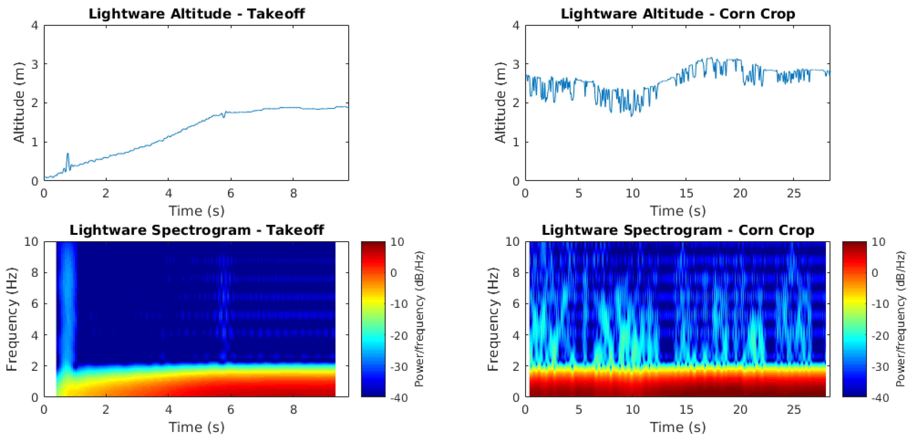
To calculate the ground truth, the data from sensors have to be filtered, in an effort to reduce the vegetation interference in the value to which each sensor is going to be compared. To be able to do this, more information about the signals was necessary to chose the frequencies of the filter to be used, thus, spectrograms were built using data in regions with and without vegetation and then compared. A spectrogram is a three dimensional representation of a signal, usually plotted as a heatmap, with the time of the signal on the horizontal axis and the FFT of the signal in a given time in the vertical axis. The color code of the heat map represents the energy of each frequency in a given time slice.
Using the unfiltered data, the ground truth is calculated using, at each sample, the average between the two sensors that are closer to each other and the standard deviation, that provides information about the dispersion of the data. The resulting values are, then, passed through a filter (using the MATLAB filtfilt function [28]) with similar specifications to the one used for the sensor data, but with a lower stopband attenuation as this is used only to remove the discontinuities caused by the calculation methodology. The data is, then, manually tagged with the aid of a video recording of the flight, split in segments corresponding to the tags and used in the error calculation stage.
The error calculation stage consists of, first calculating the MSE of the segment of each sensor in relation to the ground truth calculated as depicted in Equation (1) where MSE is the mean square error, N is the number of samples, i is the sample index, is the sensor reading, is the average of the sensors in each sample and is the error at each sample.
Then, to provide a better estimation of the error, using the data from the standard deviation of the ground truth, a modified version of the MSE is used as depicted in Equation (2) where MSEM is the Modified Mean Squared Error and it is the weighting calculated for the given error.
This error calculation function uses the standard deviation, to calculate the weight of the error as can be seen in Equation (3) where e is the Euler’s number, is the average in sample i and is the standard deviation in sample i. It uses 1 minus a gaussian function to provide a low weight for the error when it is small, and a weight of 1 when the error is big in relation to the standard deviation .
As the workflow shows, the data that is compared to the ground truth is taken right after the resampling stage. This is done to provide a comparison using the unfiltered data provided by the sensor, a situation closer to what would be the desired implementation. Since the filtfilt implementation is, by its nature, anti-causal, meaning that it cannot be implemented in an online basis, using the data filtered by it would not represent the actual result the sensors would give in a real application.
This comparison framework suffers mainly from the dependency on the data sources. Despite this fact, it is important to highlight that the final data (the ground truth reference) is actually more precise than the data provided by any sensor in the task of representing the AGL height since the combination and filtering of the data provided by the multiple sensors allows a smaller variance in the data.
5. Results and Discussion
Following the workflow presented in the Section 4, a flight was performed over the crop field started by a takeoff phase over a dirt road. The drone was, then, driven to the crop flying over plants, plantation gaps and service corridors. The culture in use in this part of the data was corn with approximately 40 days, measuring 0.5 m in average. The aircraft flies then over the dirt road and follows to a native vegetation area. This area can be separated into two regions, one of them with heights of approximately 0.3 m and another with heights of approximately 0.8 m. The data collected during this experiment can be seen in Figure 5 which shows the altitude measured by the three sensors versus time.
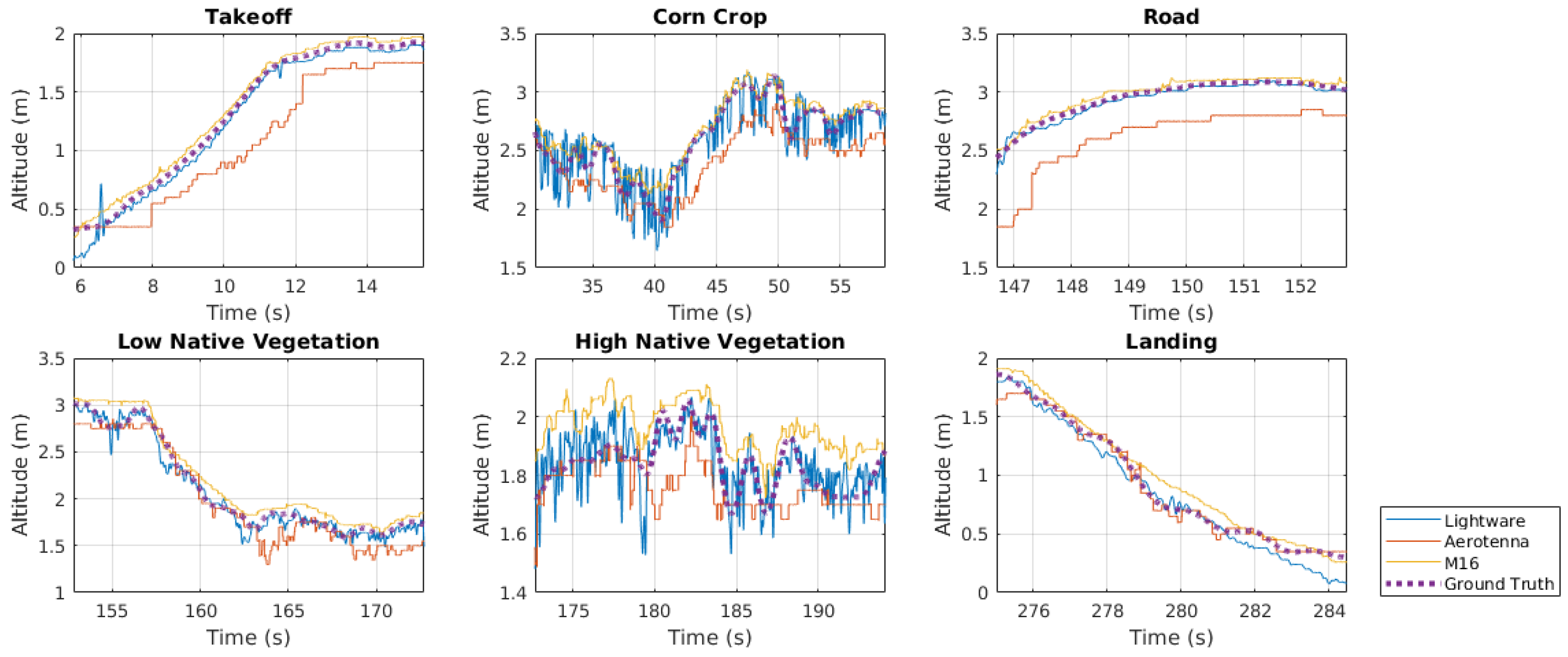
In Figure 5, it can be seen that the takeoff phase takes about 10 s (from 6 to 16 s approximately). The corn crop phase goes from 15 to 166 s approximately and includes many passages over gaps and service corridors. The flight part over the road goes from 147 to 154 s, presenting mostly a smooth surface similar to the one captured in the takeoff phase. The native vegetation pass goes from 154 to 269 s and presents a mixture of low and high plants. Those timestamps were defined using a video recording of the whole flight to tag the time markers approximately and then comparing them to the data from the sensors. Some of the tagged time periods can be seen in Figure 6. The selected time slices shown in this figure are used along the work to provide a step by step comparison.
The plot extracted from the takeoff phase shows, as expected by the smoothness of the surface, a soft ascendance on all three sensors. The corn crop extract (mainly the Lightware sensor data) clearly shows a high frequency signal overlapped with a lower frequency one. The lower frequency signal is approximately the real altitude over the plantation, while the higher frequency signal represents the texture underneath, showing accurately variations with amplitudes close to the measurements of the plants. The road and landing flight phases show similar results to the takeoff phase. The native vegetation phases do not show results as bad as the crop phase, probably because of the higher density of the plants. However, there is a clear difference in the amplitude of the oscillations between the high and the low native vegetation.
These observations were crucial to the further development of the analysis as they showed clear differences between the flight phases that can be easily recognized and characterized. To improve the understanding of the collected signals and to provide a better visual insight of the frequency content of the data, spectrograms of the three sensors under two separate conditions were built, during takeoff and over the corn crop. These plots made possible to determine the best frequency for the filter to be used in the ground truth calculation. As an example, one of these plots can be seen in Figure 7. These kind of plots were used as an attempt to provide a good visualization of the spectral content of the signals in time and with them, it was possible to see in smaller time divisions, the effect of specific phenomena. For instance, from Figure 7, it can be seen that the frequency content present in different time slices of the measurement is very different and that using the Fourier Transform alone in the whole signal from the corn crop could lead to misreading of the real contribution of the higher frequencies in the signal. This would be due to the averaging of regions that do not present the oscillations with the ones that present it. This would consequently lead to a reduction of the magnitude of the higher frequency components in the measurement with respect to the lower frequency signal (of interest), making it harder to perceive.
The altitude data followed by the spectrogram for the period of time is shown in Figure 7. On the left the data comes from the takeoff process, which took place at a very smooth surface, thus yielding to a clean signal that can be seen as a target for the filtration process. In these spectrograms, it can be seen that most of the power of the signal and, thus, most of the information of the signal is present below 2 Hz. On the right, the data comes from the section of the flight when the drone was over the crop. In this case, it can be seen that it is a signal with a much higher power in higher frequencies, as expected. Again, this is most prominent in the Lightware data. It can also be noted that around 1.5 Hz the spectrogram starts to be distorted by the crop.
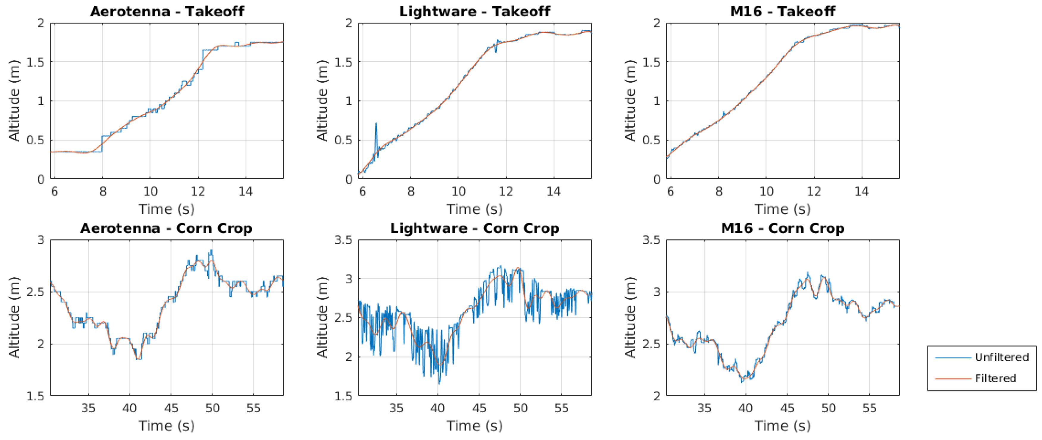
Using these observations, and after some fine tuning of the filtered results, a lowpass filter with a passband of 0.5 Hz and a stopband of 1 Hz was chosen. To avoid having distortions caused by excessive attenuation in the region of interest, the selected passband attenuation was 0.01 dB. The selected stopband attenuation was 100 dB. The window used by the filter was the Hamming window as it provides better attenuation of the side lobes, and thus, lower oscillation on the frequency response. These benefits come at the cost of a higher order filter to match the specifications. As this is an offline study and the computational power necessary for the calculations was enough not to significantly slow down the analysis, this drawback could be neglected. Figure 8 shows a comparison between the original sensor data and the filtered data.
In Figure 8, it can be seen that the data from the smooth takeoff process was not modified by the filtering, while the data from the corn crop is much cleaner, showing little influence from the texture on the ground. It is possible to highlight a fact in measuring the altitude in the corn crop phase, mainly for the Lightware sensor data: The desired altitude to be measured would be the bottom of the negative peaks as this is the altitude with relation to the plants under the drone. In this sense, this filtration enhances the results, but further improvements could be made to provide a result closer to the desired. Also, it is possible to notice that the magnitude of the signals remained mostly unchanged and there was no visible delay introduced by the filtration process.
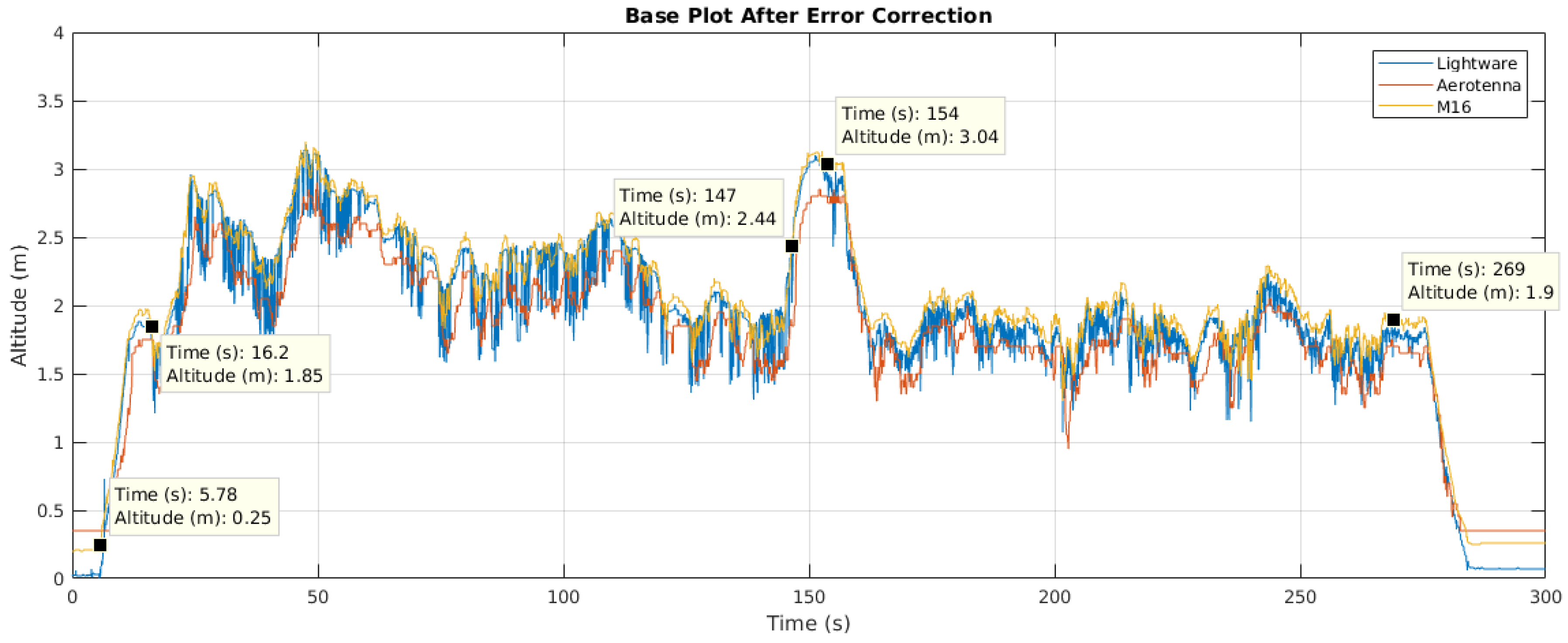
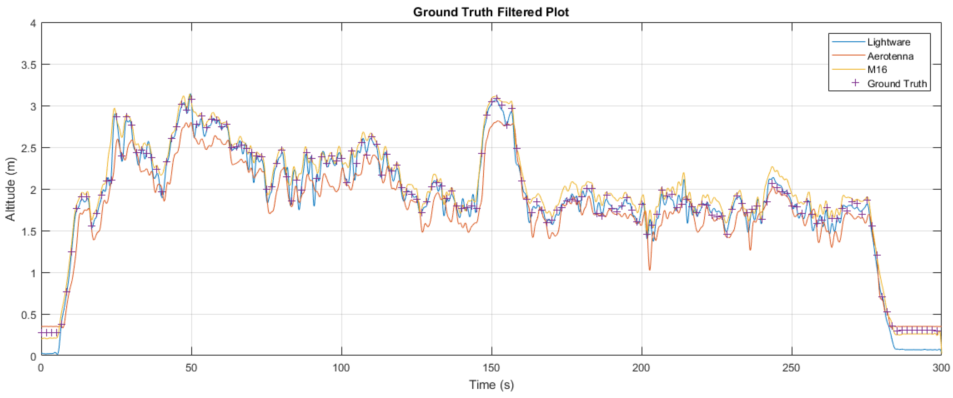
The results from the last step were then used to calculate the ground truth by using the polling system and averaging the two closest results. Still at this stage, the standard deviation could be calculated from the two nearest sensors at each time point. The resulting signal can be plotted against the filtered data from the sensors to ensure the coherence of the result and also, to provide a preliminary insight of the probable results to come from the error calculation. The plot can be seen in Figure 9 with the ground truth represented by a dashed line to improve readability. Notice that lab experiments would not help much to improve the acquired results, as the sensors work very well in controlled environments and the main goal of the work was not to determine the most precise sensor, but it was to determine the one that is less susceptible to the problems inherent to the application under concern.
As shown in Figure 9, the ground truth calculation process was correctly made and it provides coherent results. The calculated reference is seen between the sensors in all time points and follows the closest sensors. To enhance the visualization and to provide a comparison to the raw data, plots of some of the tagged regions were made. These plots can be seen in Figure 10.
Figure 9 and Figure 10 show the calculated truth to be a smooth curve that stays between the two closer sensors to each other, as designed. The effect of the filtering used to smooth the discontinuities alters the signal in a very subtle way, thus having very little influence in the end result.
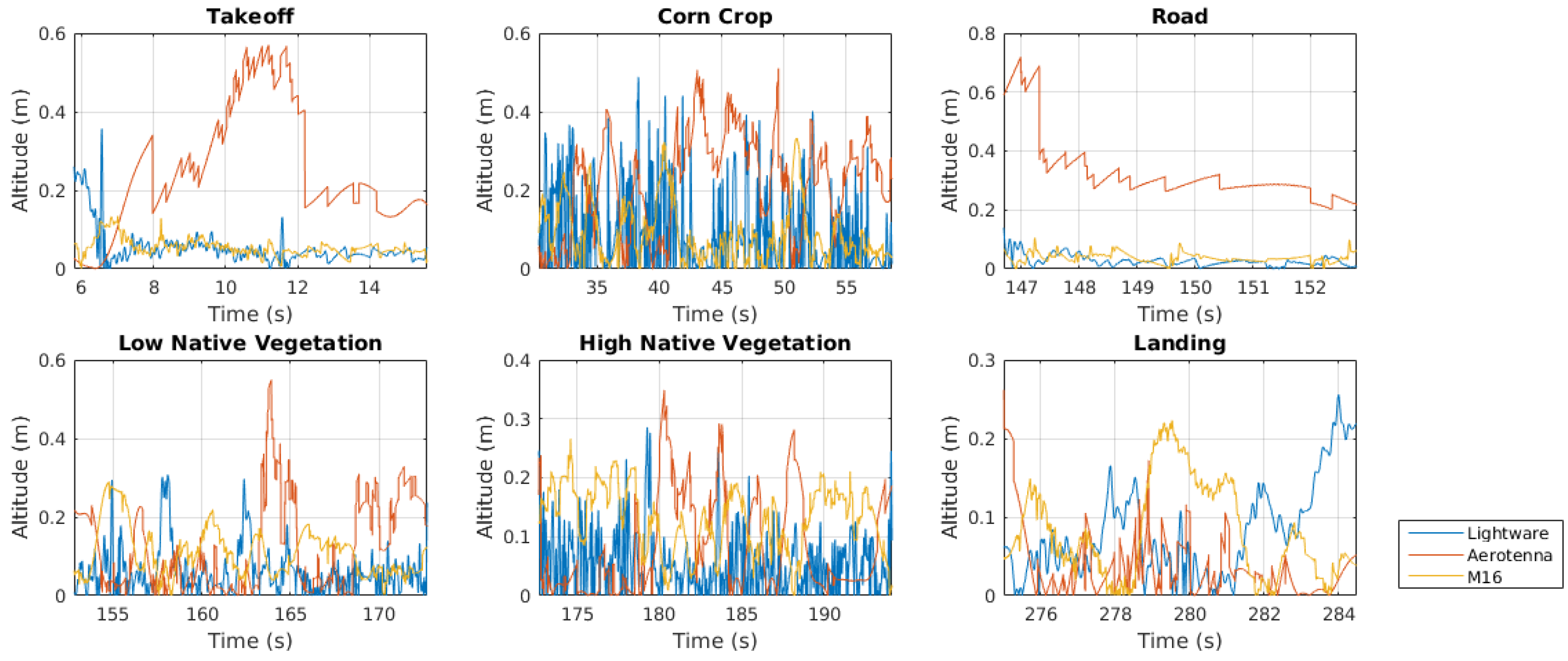
At this stage, the error plots for each sensor can be displayed to provide a graphical visualization of the accuracy of them with respect to the reference set by the ground truth. The error obtained for each sensor by subtracting its signal to the ground truth is displayed with some of the tagged periods in Figure 11.
Figure 11 already shows a trend where the Aerotenna sensor usually has the biggest error (around 0.3 to 0.4 m in most cases). This is probably due to its lack of accuracy when compared to the optical sensors (Lightware and M16). These two sensors, by the other hand show errors of less than 0.2 m in most scenarios. This error is considered to be acceptable considering the method used for estimation of the real altitude and the characteristics of the spraying process.
To enable a better visualization of the data and knowing that crop gaps and service corridors are always part of the plantation, a table accounting for this fact, summarizing the areas of flight and recalculating the MSE’s was built and is shown in Table 2. In this table, the lower the value of the MSE or of the MSEM, the smaller the overall error.
Table 2 shows that for situations where either the surface below the drone is smooth or the vegetation is dense enough, Lightware excels as the most overall accurate. In the other hand, the M16 is the most capable sensor in situations with many gaps and sparse vegetation, even without the use of more than one ray in the calculations. The Aerotenna sensor has the worse (bigger) MSE and Modified MSE indices in all of the cases. While in the laboratory, in fact, this was the most inaccurate of the sensors for static obstacles. This suggests that a process of determination of the static error of it and, possibly, magnitude adjustments in the signal provided by it, could be used to improve this sensor’s results.
The MSEM in Table 2 shown a similar result to the one seen in the MSE method. However, it can be seen that for results that are visibly closer in plots such as Figure 11, the MSEM provides a better notion of the similarity of the sensing quality provided by the sensors. This is done while still keeping the distance of already distant signals, as shown in the takeoff section. In this time slice, for the Aerotenna, which performs the worse, the MSEM shows results that are very close to the MSE, while the values for Lightware and M16 are much closer to each other, which matches with the visual perception of the data from this timestamp. This way, the MSEM can be used more effectively when deciding the right sensor for each task as it is able to provide a better differentiation of the qualities and similarities of the sensors.
From the acquired results, it is possible to highlight some learned general aspects: in situations with high sun incidence, the LeddarOne presented many problems due to the intensity of Infrared light caused by the sun, which was much stronger than the signal from the LED illuminators of the sensor. This could be extended to most LIDAR sensors to a certain degree, depending on the power of the illuminators used by each particular sensor; on the other hand, when it is known that the texture of the obstacles is rough (such as in a crop environment) it is best to use the sensor with the widest field of view available, usually provided by a RADAR or a SONAR.
6. Conclusions and Future Works
In airborne pulverization, it is essential to precisely measure the altitude of the aircraft, due to the obstacles present in the flight environment. In this sense, this work approaches the problem of altitude sensing by comparing different TOF sensors with different measuring technologies. This is done by collecting data from the sensors in a same flight and, then, developing a reference baseline to which the sensors can be compared. This was developed by the use of signal filtration, competitive algorithm and, in the end, metrics built around MSE and a modification of it are used as a basis to the decision making process.
The results shown that the Leddartech M16 and the Lightware SF11-C both perform well in different situations. The Lightware sensor excels in dense vegetation environments because of it’s superior accuracy. The much narrower divergence angle shown not to be a problem in these environments as it is hard to penetrate through the leaf thickets. The M16 is the best choice in sparser vegetation due to it’s bigger divergence angle, which captures a better averaging of the surface underneath. Additionally, its less precise measurements compared to Lightware affects very subtly its overall performance as the MSEM of the smooth ground measurements showed. This contributes to the choice for the Leddartech M16 as the best overall performer among the studied sensors, presenting the best results in most cases and in the exception cases, very similar measurements.
This study can be expanded and continued in a variety of forms. Namely, the use of the same workflow in different cultures can be of great help to improve the data basis, as in woody crops, for instance. Different environmental characteristics can still be evaluated, including the weather conditions. The influence of the suspended particles and droplets caused by the rotors of the drone and the spraying fluids needs to be analyzed quantitatively (in relation to the numerical results), but also, qualitatively, with relation to the need for maintenance and the frequency of it caused by this conditions. Improvements could be done by adding more sensors to the study, which would increase the choice basis size and also could provide improvements to the system used to calculate the ground truth, by increasing the number of competing agents. Also of great importance, it would be the execution of studies related to the collision avoidance during flight using the data from the sensors already presented in this work.
Author Contributions
C.H. defined the application; M.H., C.H. and E.P.d.F. designed the system; M.H. and E.P.d.F. designed the experiments; M.H. and C.H. performed the experiments; M.H. wrote the software and analyzed the data; I.C.G.d.V. verified the consistency of the results and wrote the paper.
Funding
Skydrones Avionics Technology financially supported the development of this work.
Acknowledgments
Thanks are expressed to the LASCAR (Control, Automation and Robotics Systems Laboratory) for the support and assistance in the preparation of this work; to Skydrones Avionics Technology for providing the structure, materials and personal. The authors thank the Brazilian Research Support Agencies CNPq and FAPERGS for granting financing support that allows the performance of this research.
Conflicts of Interest
The authors declare no conflict of interest. The founding sponsors had no role in the design of the study; in the collection, analyses, or interpretation of data; in the writing of the manuscript, and in the decision to publish the results.
Abbreviations
The following abbreviations are used in this manuscript:
| UAV | Unmanned Aerial Vehicle |
| AGL | Above Ground Level |
| AMSL | Above Mean Sea Level |
| GPS | Global Positioning System |
| RADAR | Radio Detection And Ranging |
| SONAR | Sound Navigation And Ranging |
| LIDAR | Light Detection And Ranging |
| LADAR | Laser Detection And Ranging |
| TOF | Time-of-Flight |
| COTS | Commercial-Off-The-Shelf |
| CPU | Central Processing Unit |
| IMU | Inertial Measurement Unit |
| IR | Infrared |
| RAM | Random Access Memory |
| USB | Universal Serial Bus |
| OS | Operating System |
| SD | Secure Digital |
| FIR | Finite Impulse Response |
| MSE | Mean Squared Error |
| MSEM | Modified Mean Squared Error |
| DOF | Degrees of Freedom |
| FFT | Fast Fourier Transform |
| LED | Light Emitting Diode |
References
- Spoorthi, S.; Shadaksharappa, B.; Suraj, S.; Manasa, V.K. Freyr drone: Pesticide/fertilizers spraying drone—An agricultural approach. In Proceedings of the 2017 2nd International Conference on Computing and Communications Technologies, Tamil Nadu, India, 23–24 February 2017. [Google Scholar]
- LeddarTech. LeddarTech—Technology Fundamentals; LeddarTech: Quebec City, QC, Canada, 2017. [Google Scholar]
- Sensorsinc. Sensors Unlimited-LADAR; Sensors Unlimited: Princeton, NJ, USA, 2017. [Google Scholar]
- Aerotenna. Why μLanding? Aerotenna: Lawrence, KS, USA, 2017. [Google Scholar]
- Cherian, A.; Andersh, J.; Morellas, V.; Papanikolopoulos, N.; Mettler, B. Autonomous altitude estimation of a UAV using a single onboard camera. In Proceedings of the 2009 IEEE/RSJ International Conference on Intelligent Robots and Systems, IROS, St. Louis, MO, USA, 10–15 October 2009. [Google Scholar]
- Nelson, R.C. Flight Stability and Automatic Control, 2nd ed.; Mechanical Engineering–Springer: New York, NY, USA, 1989; ISBN 978-0070462731. [Google Scholar]
- Eynard, D.; Vasseur, P.; Demonceaux, C.; Frémont, V. UAV altitude estimation by mixed stereoscopic vision. In Proceedings of the IEEE/RSJ 2010 International Conference on Intelligent Robots and Systems, IROS, Taipei, Taiwan, 18–22 October 2010. [Google Scholar]
- Moore, R.J.D.; Thurrowgood, S.; Bland, D.; Soccol, D.; Srinivasan, M.V. UAV altitude and attitude stabilisation using a coaxial stereo vision system. In Proceedings of the IEEE International Conference on Robotics and Automation, Anchorage, AK, USA, 3–8 May 2010. [Google Scholar]
- Campbell, J.P.; Blinn, J.C. Experimental Evaluation of Passive Microwave Velocity/Altitude Sensing. Water Resour. Res. 1968, 18, 1137–1142. [Google Scholar] [CrossRef]
- Cho, A.; Kang, Y.S.; Park, B.J.; Yoo, C.S.; Koo, S.O. Altitude integration of radar altimeter and GPS/INS for automatic takeoff and landing of a UAV. In Proceedings of the International Conference on Control, Automation and Systems, Venice, Itatly, 26–29 October 2011. [Google Scholar]
- Thomas, L.; Monin, A.; Mouyon, P.; Houberdon, N.E.D. Gaussian mixture filtering for data fusion with switching observation models: Application to aircraft relative altimetry. In Proceedings of the Conference on Control and Fault-Tolerant Systems, SysTol, Nice, France, 9–11 October 2013. [Google Scholar]
- Faiçal, B.S.; Pessin, G.; Filho, G.P.R.; Furquim, G.; de Carvalho, A.C.P.L.F.; Ueyama, J. Fine-tuning of UAV control rules for spraying pesticides on crop fields. In Proceedings of the 2014 IEEE 26th International Conference on Tools with Artificial Intelligence, Limassol, Cyprus, 10–12 November 2014. [Google Scholar]
- Stamatescu, G.; Stamatescu, I.; Popescu, D.; Mateescu, C. Sensor fusion method for altitude estimation in mini-UAV applications. In Proceedings of the 2015 7th International Conference on Electronics, Computers and Artificial Intelligence (ECAI), Iasi, Romania, 28–30 June 2015. [Google Scholar]
- Szafranski, G.; Czyba, R.; Janusz, W.; Blotnicki, W. Altitude estimation for the UAV’s applications based on sensors fusion algorithm. In Proceedings of the 2013 International Conference on Unmanned Aircraft Systems (ICUAS), Atlanta, GA, USA, 28–31 May 2013. [Google Scholar]
- Dandois, J.P.; Olano, M.; Ellis, E.C. Optimal Altitude, Overlap, and Weather Conditions for Computer Vision UAV Estimates of Forest Structure. Remote Sens. 2015, 7, 13895–13920. [Google Scholar] [CrossRef] [Green Version]
- Kumar, G.A.; Patil, A.K.; Patil, R.; Park, S.S.; Chai, Y.H. A LiDAR and IMU Integrated Indoor Navigation System for UAVs and Its Application in Real-Time Pipeline Classification. Sensors 2017, 17, 1268. [Google Scholar] [CrossRef] [PubMed]
- ANAC. Regras Sobre Drones—ANAC; ANAC Press: Brasilia, Brazil, 2017. [Google Scholar]
- SkyDrones. Pelicano; SkyDrones: Porto Alegre, Brazil, 2017. [Google Scholar]
- Pixhawk.org. Pixhawk Series Documentation; Pixhawk: Zurich, Switzerland, 2018. [Google Scholar]
- Optoelectronics, Inc. SF11 Laser Altimeter Product Manual; Optoelectronics, INC.: Boca Raton, FL, USA, 2016. [Google Scholar]
- LeddarTech. Leddar One Fact Sheet; LeddarTech: Quebec City, QC, Canada, 2017. [Google Scholar]
- LeddarTech. Leddar Sensor Module User Guide; LeddarTech: Quebec City, QC, Canada, 2015. [Google Scholar]
- Raspberry Pi Foundation. Raspberry Pi; Raspberry Pi Foundation: Cambridge, UK, 2017. [Google Scholar]
- Long, J.P. Complete Guide for Python Programming: Quick & Easy Guide to Learn Python; CreateSpace: Scotts Valley, CA, USA, 2015. [Google Scholar]
- TE Connectivity. MS5611-01BA03; TE Connectivity: Schaffhausen, Switzerland, 2017. [Google Scholar]
- Liu, H.; Pang, G. Accelerometer for Mobile Robot Positioning. IEEE Trans. Ind. Appl. 2017, 37, 812–819. [Google Scholar] [CrossRef]
- Aishwarya, B.B.; Archana, G.; Umayal, C. Agriculture robotic vehicle based pesticide sprayer with efficiency optimization. In Proceedings of the 2015 IEEE International Conference on Technological Innovations in ICT for Agriculture and Rural Development, TIAR, Chennai, India, 10–12 July 2015. [Google Scholar]
- Hahn, B.H.; Valentine, D.T. Essential MATLAB for Engineers and Scientists, 6th ed.; Academic Press Elsevier: London, UK, 2017; ISBN 978-0-08-100877-5. [Google Scholar]
Figure 1.
Class 3 RPA Pelicano.
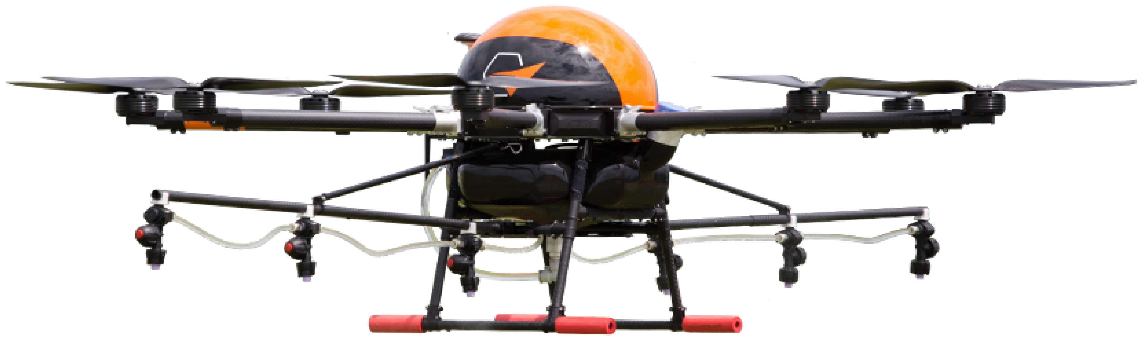
Figure 2.
Stand (a) and drone with the sensors (b).

Figure 3.
Data acquisition diagram.

Figure 4.
Analysis workflow.

Figure 5.
Raw data before filtering.

Figure 6.
Timestamps zoomed.
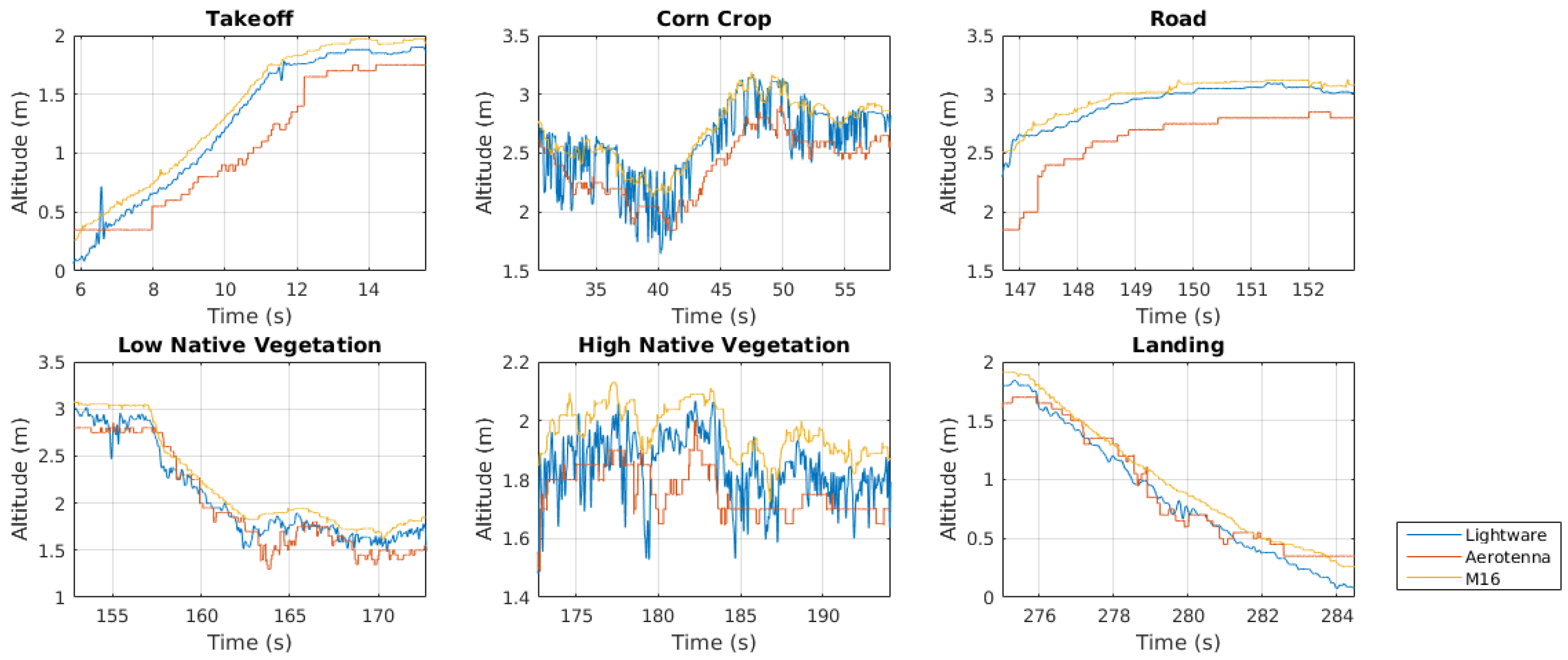
Figure 7.
Spectrogram—Lightware.

Figure 8.
Comparison between filtered and unfiltered data.

Figure 9.
Ground Truth.

Figure 10.
Ground Truth zoom.

Figure 11.
Error Plot Zoomed.

Table 1.
Sensor Specifications.
| Sensor | Lightware SF11-c | LeddarTech LeddarOne | LeddarTech M16 | Aerotenna Landing |
|---|---|---|---|---|
| Approximate Cost | U$ 300 | U$ 100 | U$ 750 | U$ 500 |
| Alias for the sensor | “Lightware” | “LeddarOne” | “M16” | “Aerotenna” |
| Technology | LADAR | LIDAR | LIDAR | RADAR |
| # Rays | 1 | 1 | 16 | 1 |
| Aperture () | 0.2 | 3 | 95 | 20 × 30 |
| Sensing Rate (Hz) | 20 | 140 | 1.56–100 | 800 |
| Accuracy (m) | ±0.1 | 0.05 | ±0.05 | 0.05 |
| Resolution (m) | 0.01 | 0.03 | 0.01 | 0.01 |
| Min. Range (m) | 0.1 | 0 | 0 | 0.32 |
| Max. Range (m) | 120 | 40 | 100 | 45 |
| Interface | RS-232 | Proprietary-USB | Proprietary-USB | RS-232 |
| Wavelength (nm) | 905 | 850 | 940 | 12.5 × 10⁶ |
Table 2.
Error Summary.
| Duration (s) | Flight Phase | MSE (m2) | MSEM (m2) | ||||
|---|---|---|---|---|---|---|---|
| Aerotenna | Lightware | M16 | Aerotenna | Lightware | M16 | ||
| 31.4 | Smooth Ground | 0.0553 | 0.0052 | 0.0063 | 0.0518 | 0.0036 | 0.0038 |
| 131.1 | Corn Crop | 0.0564 | 0.0177 | 0.0144 | 0.0531 | 0.0147 | 0.0108 |
| 86.6 | High Native Vegetation | 0.0256 | 0.0089 | 0.0176 | 0.0211 | 0.0066 | 0.0136 |
| 29.6 | Low Native Vegetation | 0.0344 | 0.0054 | 0.0127 | 0.0295 | 0.0033 | 0.0091 |
© 2018 by the authors. Licensee MDPI, Basel, Switzerland. This article is an open access article distributed under the terms and conditions of the Creative Commons Attribution (CC BY) license (http://creativecommons.org/licenses/by/4.0/).
Share and Cite
MDPI and ACS Style
Hentschke, M.; Pignaton de Freitas, E.; Hennig, C.H.; Girardi da Veiga, I.C. Evaluation of Altitude Sensors for a Crop Spraying Drone. Drones 2018, 2, 25. https://doi.org/10.3390/drones2030025
AMA Style
Hentschke M, Pignaton de Freitas E, Hennig CH, Girardi da Veiga IC. Evaluation of Altitude Sensors for a Crop Spraying Drone. Drones. 2018; 2(3):25. https://doi.org/10.3390/drones2030025
Chicago/Turabian StyleHentschke, Matheus, Edison Pignaton de Freitas, Carlos Henrique Hennig, and Igor Caike Girardi da Veiga. 2018. "Evaluation of Altitude Sensors for a Crop Spraying Drone" Drones 2, no. 3: 25. https://doi.org/10.3390/drones2030025