UAS Navigation with SqueezePoseNet—Accuracy Boosting for Pose Regression by Data Augmentation


Institute of Photogrammetry and Remote Sensing (IPF), Karlsruhe Institute of Technology (KIT), D-76131 Karlsruhe, Germany
*
Author to whom correspondence should be addressed.
Drones 2018, 2(1), 7; https://doi.org/10.3390/drones2010007
Submission received: 20 December 2017
/
Revised: 24 January 2018
/
Accepted: 5 February 2018
/
Published: 13 February 2018
(This article belongs to the Special Issue Latest Developments, Methodologies and Applications Based on UAV Platforms)
Abstract
:The navigation of Unmanned Aerial Vehicles (UAVs) nowadays is mostly based on Global Navigation Satellite Systems (GNSSs). Drawbacks of satellite-based navigation are failures caused by occlusions or multi-path interferences. Therefore, alternative methods have been developed in recent years. Visual navigation methods such as Visual Odometry (VO) or visual Simultaneous Localization and Mapping (SLAM) aid global navigation solutions by closing trajectory gaps or performing loop closures. However, if the trajectory estimation is interrupted or not available, a re-localization is mandatory. Furthermore, the latest research has shown promising results on pose regression in 6 Degrees of Freedom (DoF) based on Convolutional Neural Networks (CNNs). Additionally, existing navigation methods can benefit from these networks. In this article, a method for GNSS-free and fast image-based pose regression by utilizing a small Convolutional Neural Network is presented. Therefore, a small CNN (SqueezePoseNet) is utilized, transfer learning is applied and the network is tuned for pose regression. Furthermore, recent drawbacks are overcome by applying data augmentation on a training dataset utilizing simulated images. Experiments with small CNNs show promising results for GNSS-free and fast localization compared to larger networks. By training a CNN with an extended data set including simulated images, the accuracy on pose regression is improved up to 61.7% for position and up to 76.0% for rotation compared to training on a standard not-augmented data set.
1. Introduction
More and more Unmanned Aerial Vehicles (UAVs) are operating in industrial, research and private areas, leading to a growth of interest in UAV-related topics such as navigation, data acquisition, path planning or obstacle avoidance. For UAV positioning, general opposite items are of interest and described:
- Global Referencing vs. Local Referencing
- High Computational Power vs. Low Computational Power
- Hand-made Features vs. Learned Features
- Multi-View Stereo vs. Pose Regression
Unmanned Aerial Systems (UASs) need reliable navigation solutions for Global Referencing which are mostly based on GNSS and often combined with Inertial Navigation Systems (INSs). As failures, due to gaps in signal coverage caused by occlusions or multipath effects, weaken satellite-based navigation, alternative methods for a reliable navigation of Unmanned Aerial Systems are mandatory. One of those state-of-the-art methods is aerial image matching based on feature detection or correlation which are used for navigational purposes. These methods are computational intensive, especially for navigating in large areas where a vast number of descriptors potentially has to be stored and matched. Further methods for navigating in a global reference frame, are commonly based on digital surface models, digital terrain models or CAD models [1]. However, the large memory consumption of such models renders this approach infeasible for on-board processing on computational weak computers which are commonly mounted on UAVs.
Global referencing is commonly aided by Local Referencing to bridge gaps and maintain a continuous navigation. Local navigation methods such as visual Simultaneous Localization and Mapping (SLAM) or Visual Odometry (VO) are potential techniques for reconstructing trajectories [2,3,4]. Considering additional information, such as geo-referenced key points or initialization to a referenced model, allows global referencing for local navigation methods. Nevertheless, for short frame-to-frame distances, these methods score high accuracies. Drawbacks are drift effects for longer distances caused by cumulative errors. However, these local solutions can potentially support global navigation algorithms in a complementary way. Visual SLAM or VO fail once the pose estimate is lost which can be caused by fast motions or occlusions. Global re-localization methods could be used to recover the pose in such cases. However, global navigation methods are capable as standalone systems.
While most navigation methods work fine on computers with High Computational Power, running them on weak or embedded devices with Low Computational Power may lead to limited real-time capability or even failures. Running a navigation framework on small UAVs or Micro Aerial Vehicles (MAVs) limits the computation power due to maximum payload. Therefore, all developed methods are subject to the limited computational power of the on-board processing units and need to be carefully designed with the target hardware in mind. A potential solution may be provided by Convolutional Neural Networks which need high computational power during the training step, but only a fraction of that during runtime. CNNs can perform fast forward passes even on small on-board GPUs and have a limited memory demand and power consumption [5]. Therefore, CNNs offer a valuable solution for on-board computers.
Pose estimation with deep CNNs based on Learned Features, such as PoseNet [6] has been shown recently. CNNs solve image matching tasks, where Hand-made Features such as Scale Invariant Feature Transform (SIFT) [7], Oriented FAST and rotated BRIEF (ORB) [8] or Speeded Up Robust Features (SURFs) [9] might fail due to less descriptive features. However, a satisfying solution for VO using CNNs trained end-to-end is not yet available. For the demands on UAV navigation, the utilization of a small CNN that can be used on-board computers is mandatory. Therefore, a CNN-based solution for the navigation or localization of an UAV in a known environment is utilized by SqueezePoseNet [10].
Data augmentation became an important element, overcoming problems in several fields of computer vision. The success of training-based methods such as CNNs and the coexisting lack of training data increased the value of data augmentation even more. Modification of existing training data as well as the simulation of purely new data are used to augment training sets. Therewith, training classifiers or regressors became very successful by utilizing the diversity of modified, synthesized or simulated data.
The main contribution of this submission, besides SqueezePoseNet, is the investigation on data augmentation on training sets to improve Pose Regression by CNNs. For this purpose, a training data set is extended with simulated images. Therefore, a photo-realistic 3D model of the environment is generated. This 3D model serves for rendering images with arbitrary poses in the environment which augment and enrich the original training data set. Further, the pose results are approved with a standard Multi-View Stereo approach for evaluation.
The paper is structured as follows. After reviewing related work on pose determination, navigation methods, CNNs and data augmentation in Section 2 (Related Work), the modification of CNNs to solve for pose regression as well as the approach of accuracy boosting by data augmentation is investigated in Section 3 (Methodology). The training process on different data sets is further described in Section 4 (Training). In Section 5 (Data), the benchmark data set Shop Façade and the captured data set Atrium utilized for this work are presented. Furthermore, the Puzzle data set is introduced for the approach on data augmentation. The Unmanned Aerial Vehicle as well as the hardware used for data acquisition is specified in Section 6 (Unmanned Aerial System); Experiments on pose regression by PoseNet, a modification of the VGG16-Net and SqueezePoseNet are carried out on the mentioned data sets in Section 7 (Experiments). The results are presented numerically and visually and subsequently interpreted in Section 8 (Discussion). Finally, Section 9 (Conclusion and Outlook) summarizes the findings of the paper and provides ideas for future work and research.
2. Related Work
The determination of camera poses from images in a global coordinate frame is a useful and wide-ranging task. Solutions for this purpose are provided by finding correlations between aerial and UAV images for image matching and further localization of aerial vehicles [11,12]. Feature-based methods successfully match remotely sensed data [13,14] or oblique images [15]. Such feature-based methods often suffer from mismatches which is effectively tackled by Locality Preserving Matching (LPM) [16]. Alternatives to determine camera poses from imagery are model-based approaches [17,18]. Determining the camera pose in real time, in indoor environments, is practicable by CAD model matching [19,20,21,22]. Convolutional Neural Networks are used to determine matches between aerial images and UAV images [23] or terrestrial images and UAV images [24].
However, these methods are not operable on small drones in large environments, due to the on-board computers’ limited storage.
Feasible methods to conduct local navigation are visual SLAM or VO approaches, reconstructing a trajectory based on image sequences. Efficient solutions are ORB-SLAM [4], Large-Scale Direct Monocular SLAM (LSD-SLAM) [3] or Direct Sparse Odometry (DSO) [2]. These methods provide satisfying solutions according to accuracy and real-time capability. However, their trajectory will only be based on a local reference. Navigating in higher level coordinate frames can be achieved by fusing local solutions with, for instance, GNSS or other global localization methods. Even though SLAM or VO solutions show impressive results (e.g., DSO) and drift only slightly for short trajectories, they will certainly drift over long distances, particularly if there are no loop closures. Additionally, SLAM or VO methods fail once the track is lost. Restoring the lost track is impossible without moving back to a known or mapped position.
Therewith, local and global navigation approaches build a complementary framework, merging the advantages of both systems. The satisfying accuracy of relative pose estimations derived from neighboring frames and the computational speed of local methods as well as the global referencing to counter drift and trajectory losses are mutually supportive.
A part of this work is based on PoseNet [6], a Convolutional Neural Network which re-localizes an acquired image in a known area. The CNN is trained with images and their corresponding poses in order to estimate the pose of an unknown camera during test time. The CNN estimates poses between two trained images by regression, but also extends the learned information to determine poses which slightly exceed the trained space. However, these results suffer concerning spatial accuracy. An enhancement to the original PoseNet is the Bayesian PoseNet [25] which provides re-localization uncertainty by adding dropout layers after each convolutional layer and improves the PoseNet accuracy by averaging over multiple forward passes. For large-scale data sets (e.g., King’s College, 5600 m2) PoseNet scores approximately 2 m and 3° for mean pose estimates. PoseNet was originally built on GoogLeNet [26], a CNN designed for classification tasks, as the ImageNet Large Scale Visual Recognition Challenge (ILSVRC). However, the feasibility of pose regression with CNNs is shown in earlier works [6]. Enhanced accuracies in the task of estimating poses were derived by further improvement [27] using Long Short-Term Memory layers (LSTM) [28], a type of recurrent neural net which was combined with CNNs in the past. LSTMs handle the problem of a dissolving gradient during the back-propagation using so-called gates. However, they showed great success in handwriting or speech recognition and recently in image re-localization. Furthermore, to improve a potential navigation approach, one may support the input of a CNN with additional data. Combining RGB data and depth data in a dual stream CNN showed further improvements of the localization results [29].
Considering that deep CNNs with a large number of parameters need a higher computation power than smaller CNNs, the latter is preferred for UAV applications. For example, the VGG16-Net [30] has 528 MB of weights which will exceed the capacity of an on-board processing unit such as DJI Manifold which is used for development (Section 6.2). The model size of PoseNet or the LSTM-based CNN which are based on GoogLeNet have sizes of about 50 MB. However, due to the modification of some layers for pose regression, the number of weighting parameters increases and therefore the net sizes vary slightly. A CNN that is small enough to run on an on-board processing unit while maintaining sufficient accuracy is mandatory. SqueezeNet [31], for instance, is a small CNN with a data size of only 4.8 MB which is ten times smaller than GoogLeNet. In future work, this might be reduced even more by quantization [32] or binarization [33].
Furthermore, pose regression may potentially be improved by data augmentation. Improving the performance of classifiers and CNNs by augmenting training data sets is widely known and well established [34,35,36,37]. Common data augmentation methods are to shift, rotate, scale, flip, crop, transform, compress or blur the training images to extend the training database. This supports classifiers and CNNs to learn invariance to, e.g., shifts and rotations, which helps to generalize and increase accuracy [38,39]. Simulated or synthetic images rendered from 3D models have long been used in computer vision to generate even more extensive training data [40,41]. Rendering images from 3D objects is also practised to expand training data and improve the performance of CNNs [42,43]. To render images for pose regression demands, a 3D model of the target environment is necessary. Generating 3D models is of great interest in research communities such as photogrammetry, computer vision or geo-information sciences [44,45,46]. Research focuses on the reconstruction of such models and its automation [46,47,48]. Moreover, recently, various benchmark data sets for visual localization and with varying conditions have been published [6,49].
3. Methodology
The methodology is divided into two sections. The modifications applied on CNNs to solve for pose regression are described in Section 3.1. Subsequently, the data augmentation approach to increase accuracy is outlined in Section 3.2.
3.1. Modifications of CNNs
For the demands on pose regression SqueezePoseNet [10], an adaptation of SqueezeNet [31] is utilized. Whereas SqueezeNet is designed for solving classification tasks, SqueezePoseNet is modified to solve for pose regression. The architecture of SqueezePoseNet is depicted in Figure 1. A fully connected layer with 500 neurons is added after the last pooling layer. For pose estimation, two fully connected layers (Position and Rotation) with 3 and 4 neurons, respectively, were added. SqueezeNet’s originally design strategy consists of multiple Fire modules. Each Fire module first decreases the number of input channels from the previous layer by 1 × 1 convolutions in a so-called squeeze operation. Subsequently, an expand operation that is a combination of 1 × 1 and 3 × 3 filters increases the number of activation maps but keeps the number of parameters low (Figure 2).
In addition, the traditional SqueezeNet architecture lacks a final fully connected layer as these layers increase the number of parameters significantly. Instead, the final convolutional layer consists of as many 1 × 1 filters as classes. Subsequently, average pooling is used to yield a vector whose length equals the number of classes. To modify SqueezeNet’s architecture for pose regression, a fully connected layer with 500 neurons is introduced. This layer acts as a descriptor and is meant to help the network distinguish different poses from each other. Additionally, the layer’s activation functions are changed from Rectified Linear Units (ReLUs) to Leaky Rectified Linear Units (Leaky ReLUs) [50]. This is meant to help convergence. In addition, Batch Normalization [51] is added after each convolutional layer, making higher learning rates possible. Finally, two fully connected layers for actual pose estimation were added. A three-neuron layer for position and a four-neuron layer for rotation. The rotation is parametrized as a quaternion. The training is described in Section 4.
For the purpose of evaluation, a deeper Neural Network, the VGG16-Net [30], is modified to compare it with the smaller SqueezePoseNet. Deeper networks obviously tend to be more accurate than small ones [31]. The modification on the VGG16-Net was realized the same way as the modification on SqueezeNet. Two dense layers (Position and Rotation) for pose regression were added and the layer’s activation functions were set to Leaky Rectified Linear Units.
CNNs are optimized by iteratively changing their weighting parameters using back-propagation. To optimize SqueezePoseNet for pose regression, the following loss [6] is minimized:
The loss is calculated as the sum of the position error and the weighted orientation error. and are ground truth and estimated position in metric dimensions. and are ground truth and estimated orientation in quaternions. Since position and orientation are not in the same unit space and therefore are not comparable, a weighting is done by using to keep the errors in the same range. This prevents the CNN from minimizing only one of the two error values. Typically, is set between 250 and 2000 for outdoor data sets. For the experiments, is set to 500.
3.2. Data Augmentation
To improve the net’s performance, data augmentation is used, whereas a training data set is extended with simulated images and their corresponding poses. Therewith, the CNN should be able to learn the appearance of images and their poses in more extended space according to the original training data. For this approach to enhancing the performance of a CNN, simulated images were added to an existing image data set. Rendering additional images to extend the data set presumes that a 3D model of the target environment is existent. This is obtained without the need of additional data by only utilizing the original image data set to generate a photo-realistic model of the environment. For this purpose, a standard multi-view stereo approach [52] is used to generate textured 3D models from images. Automatic feature extraction and feature matching is performed to compute poses of the training images. By finding further correspondences, a 3D model is generated. The model’s texture is created automatically from the training images. No additional data, aside from the training data set, is needed for this approach. Since the textures of the model are created directly from the input images, a photo-realistic model is generated. For generating simulated images, the Gazebo simulator [53] is utilized to render images with arbitrary perspectives to extend the Puzzle training data set.
4. Training
Convolutional Neural Networks usually need a huge amount of training data to perform well, which is often not accessible. Transfer-learning is a valuable process to overcome this issue. For that, a net is initially pre-trained with a huge amount of data, which is often publicly available, to determine weights for the net’s layers. These weights are used as initial values for later training.
SqueezeNet is initialized with weighting parameters trained on the ImageNet data set [54]. It was shown that for pose regression, training on the Places data set [55,56] leads to further improvement in terms of accuracy [6], as it is a more suitable data set for pose regression. Training was subsequently carried out on the Places data set.
Before starting training for pose regression on the re-localization data set Atrium (Section 5.2), SqueezePoseNet was pre-trained on the Shop Façade benchmark data set (Section 5.1). However, only the added layers were set as trainable (the last three fully connected layers in Figure 1), since the preceding layers should already be well initialized by the pre-training steps. After training the network on the Shop Façade benchmark, the CNN is finally fine-tuned on the training data of the Atrium data set consisting of 864 images. The inputs for the CNNs are 757 training images and 95 testing images with their corresponding camera poses. The training on SqueezePoseNet ended with errors of 4.45 m for position and 14.35° for orientation.
For accuracy evaluation of SqueezePoseNet, the deeper VGG16-Net, which should be more accurate, was chosen. Considering that VGG16-Net is built to solve classification tasks, it is adapted in a similar manner as SqueezeNet described above to estimate poses. The net’s layers were initialized with weights obtained by training on the Places365 data set. The adaptation is also trained on Shop Façade to obtain initial weights for the added layers. The modified net is then trained on the data set Atrium. The training errors result in 2.35 m and 9.09° for position and rotation, respectively.
To show the benefit of the utilization of data augmentation by simulated images, an additional training was carried out with the original Puzzle training dataset and the dataset extended with 479 simulated images. Furthermore, to preserve comparable results, performance evaluation was realized on two Convolutional Neural Networks: the original PoseNet and the VGG16-Net modified for pose regression. Note that the focus is on relative performance improvements of the net’s accuracy, not on the absolute accuracy itself. The training process with the initial Puzzle data set (without any simulated images) of PoseNet ended in training errors of 0.13 m and 6.00°; VGG16-Net training ended with training errors of 0.20 m and 5.00°. The training with the added 479 simulated images ended for PoseNet with a training error of 0.18 m and 6.44° and for VGGG16-Net net with 0.04 m and 1.98° respectively.
To summarize, the work flow of the methodology can be described as follows. (i) Choose a suitable CNN for classification tasks; (ii) Initialize the CNN with pre-trained weighting parameters; (iii) Transfer learning on a suitable data set, e.g., Places (optional); (iv) Prepare the CNN to solve for pose regression by adding appropriate layers; (v) Produce training data for a target environment. Optionally, the training data set could be extended by data augmentation; (vi) Train the network (the trainable layers are restricted to the last fully connected layers); (vii) Train the CNN with own training data; (viii) Run the CNN on evaluation images.
All training procedures were carried out on a 64 GB RAM computer equipped with an Intel® Core™ i7-3820 3.6 GHz processor and an 8 GB GeForce GTX 980 graphics card.
5. Data
In this section, the benchmark data set Shop Façade (Section 5.1) and the captured data set Atrium (Section 5.2) that are used for training and evaluation of the Convolutional Neural Networks for pose regression are described. Besides, the ImageNet and Places data sets serve for pre-training. The experiments on data augmentation for pose regression are carried out on the Puzzle data set (Section 5.3).
5.1. Shop Façade Data Set
The Shop Façade data set is part of the Cambridge Landmarks benchmark [6]. This outdoor data set for visual re-localization contains three video sequences recorded with a smartphone camera and their extracted image frames separated in 231 training and 103 evaluation images. A pose is provided for every image. The modified CNNs are trained on Shop Façade to yield initial weighting parameters for further training on the Atrium data set. The data set containing image sequences and poses of Shop Façade (available online http://mi.eng.cam.ac.uk/, accessed on 14 December 2017)). The dimension of the area in which the images were captured is denoted as 35 m × 25 m.
5.2. Atrium Data Set
The Atrium data set consists of 864 images collected within the LaFiDa (available online https://www.ipf.kit.edu/lafida.php, accessed on 14 December 2017)) benchmark collection by KIT [57]. These images in high resolution (available online https://www2.ipf.kit.edu/pcv2016/downloads/ photos_atrium_recon-struction.zip, accessed on 14 December 2017)) are used to determine the poses with Agisofts Structure from Motion (SfM) routine [58]. For introducing the Atrium environment, side views of the 3D model are shown in Figure 3a,b. The dimension of the captured area (39 m × 36 m × 18 m) is similar to the Shop Façade environment, at least for the ground area.
Two image sequences of the Atrium serve for evaluation. The images of the medium coverage sequence are captured in a low altitude and are spatially close to the training data. The images of the low coverage sequence are spatially far away and have high discrepancies in perspectives compared to the training data. However, the medium coverage sequence includes 145 extracted images, which show medium coverage of the training data. High coverage can be stated, if training and testing data show very similar poses. The low coverage sequence is captured with a higher altitude than the medium coverage sequence and shows low coverage of the training data, as no images with high altitude or a downward facing field of view are present in the training images. Therefore, the positions as well as the orientations are ‘far away’ from the training poses. However, the low coverage sequence is challenging for a Convolutional Neural Network, as it has not learned similar images nor poses during the training process. Ground truth is built by adding the evaluation images to the Structure from Motion (SfM) pipeline to determine their poses. For evaluation, the received poses serve as ground truth and are used to compute differences to the corresponding camera poses estimated by the CNN.
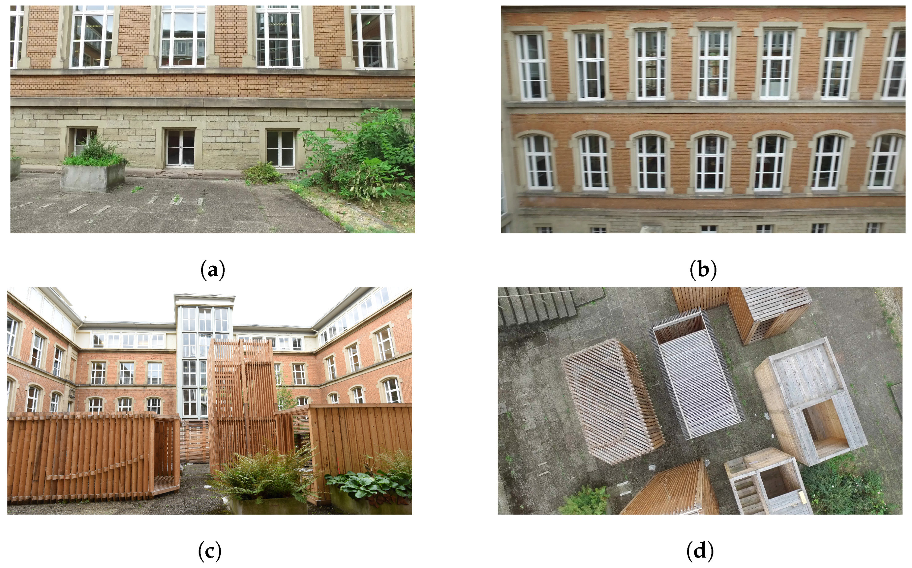
Figure 4 shows examples of training and testing images. Figure 4a shows a test image where reflections could be detected. Figure 4b shows a blurred image caused by angular motion of the UAV. Both effects are known for challenging computer vision tasks. Figure 3 and Figure 4c show the very ambiguous structures on the Atriums walls. Figure 4d shows a test image of the low coverage sequence. A similar image is not contained in the training data. The position as well as the orientation are very far away from any training pose.
5.3. Puzzle Data Set
This data set assists the investigation by showing how data augmentation can improve the accuracy of CNNs on pose regression. The simplicity of this data set serves to show the feasibility of a data augmentation approach and reduces visualization difficulty. The performance of CNNs is evaluated on the original Puzzle data set and on the Puzzle data set augmented with simulated images. The standard Puzzle data set consists of 19 images captured in nadir perspective of a puzzle. The nadir images were captured to recreate an aerial image-like scene. Therefore, these images could be compared to an aerial flight to collect spacious training data. Additionally, the data set consists of 48 test images captured closer to the puzzle and in oblique perspectives. These images represent images taken within an UAV-flight in lower altitude. The test images serve for evaluation purposes. The spatial extents of the puzzle are 114.3 cm × 82.6 cm. These metric dimensions do not match a real-world scenario. However, this is not crucial for the CNNs’ work flow and outcome, since the weighting parameter handles scale differences. Additionally, for later evaluation, not the absolute metric measurements, but the ratio between the metric results compared to the spatial extent of the target 3D environment is of primary interest.
The 19 data set images serve for generating a photo-realistic 3D model (Figure 5).
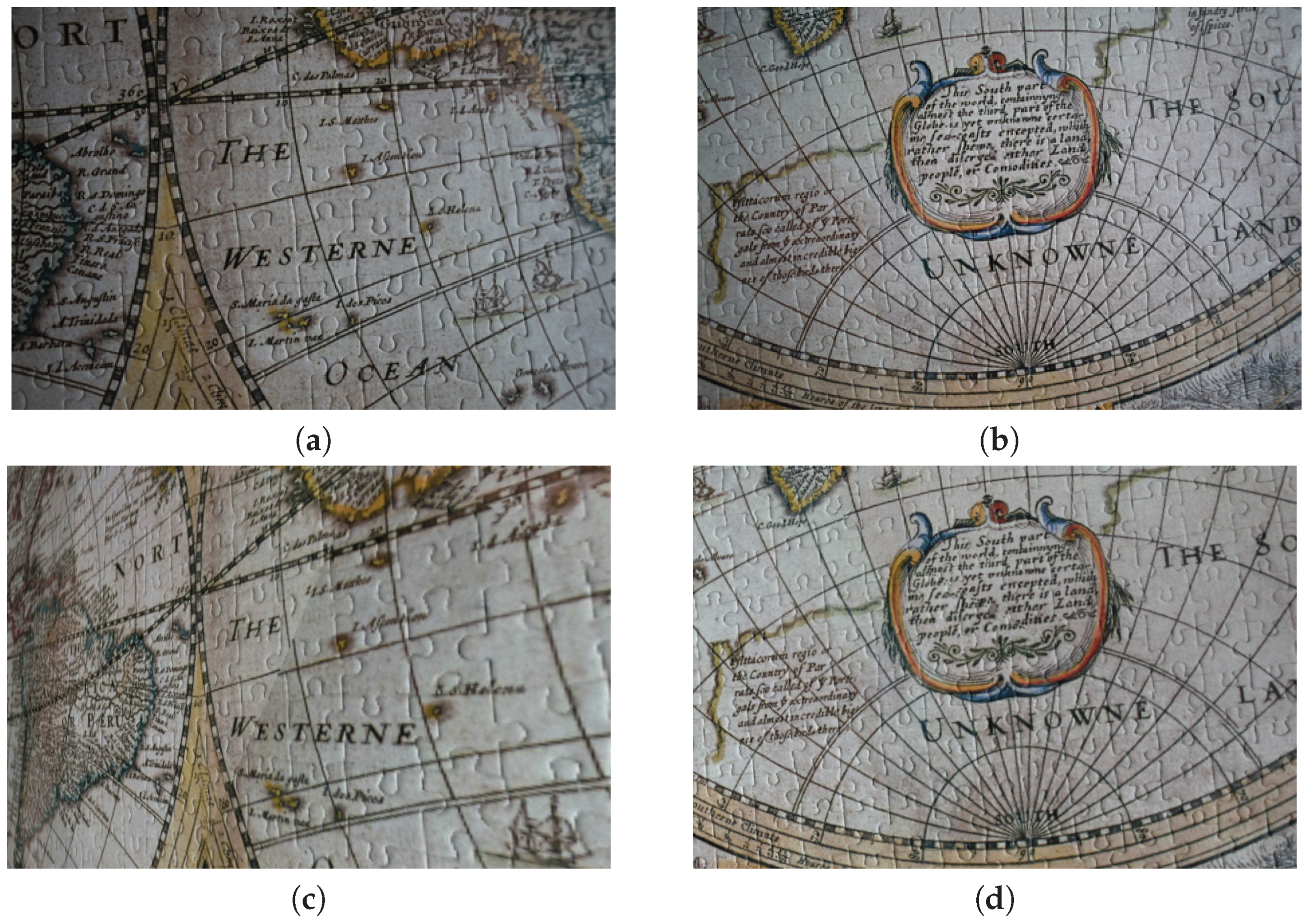
To extend the Puzzle data set, 479 images of different perspectives of the model were rendered and added to the data set. The Puzzle data set, after data augmentation therefore consists of 498 images in total. The correctness of rendered images was visually verified as visualized in Figure 6. The figure shows two real-world images in the top row and their corresponding simulated images from the photo-realistic model in the bottom row. Note that the pose of Figure 6a is determined incorrectly within the SfM process, which leads to a faulty rendered Figure 6c. The pose of Figure 6b is determined correctly, whereby the corresponding model Figure 6d is rendered accordingly.
6. Unmanned Aerial System
This Section presents an overview of the Unmanned Aerial System (UAS), which mainly consists of a UAV (Section 6.1), an on-board processing unit (Section 6.2) and a camera (Section 6.3).
6.1. Unmanned Aerial Vehicle
A Matrice 100 from DJI (Dà-Jiāng Innovations Science and Technology Co., Ltd: Skyworth Semiconductor Design Building, No.18, Gaoxin South 4th Ave, Nanshan District, Shenzhen, China, 518057) (Figure 7) and the X3 camera (Section 6.3) serve to capture images for the experiments (Section 7). The on-board processing unit, a DJI Manifold (Section 6.2) is used for data storage. Besides, it is capable of running the proposed SqueezePoseNet. The quadrocopter is able to carry about 1 kg of payload with a maximum take off weight of 3600 g. The training of the CNNs is processed offline; only the actual re-localization or navigation process has to be processed on-board.
6.2. On-Board Processing Unit
The DJI Manifold, shown on top of the UAV in Figure 7, is based on a NVIDIA® Tegra K1 with a Quad-core Arm® Cortex A-15 32-bit processor. The Kepler GPU consists of 192 CUDA® cores. CUDA® is NVIDIAs® software architecture to process computations on a Graphics Processing Unit (GPU) which is necessary for most deep learning tasks. Furthermore, the Manifold is compatible with cuDNN®, NVIDIAs® GPU-based deep neural network library, which includes standard routines for CNN-processing and CNMeM, a memory manager for CUDA. Besides, the DJI Manifold has 2 GB of RAM. With SqueezePoseNet, it is possible to process pose regression in real time. The weight of the device is less than 200 g.
6.3. Camera
The UAV is equipped with a DJI Zenmuse X3 camera, shown on the bottom of the UAV in Figure 7. It is capable of taking single shot images with a resolution of 4000 × 2250 pixels or capturing video streams with a resolution of 3840 × 2160 pixels and 30 frames per second. The camera has a 1/2.3” CMOS sensor (6.2 mm × 4.6 mm) with 12.4 megapixel. Its field of view is 94°. The camera and its gimbal weigh 254 g.
7. Experiments
For the experiments, the pose estimations derived by CNNs are evaluated by Multi-View Stereo [52,58]. SqueezePoseNet is evaluated on the medium and low coverage sequences mentioned in Section 5.2. For comparison, the VGG16-Net adaptation and PoseNet [6] are also evaluated on these two sequences. In Section 7.1 and Section 7.2, visual results as well as metric evaluations against ground truth are shown. The experiments on data augmentation on the Puzzle data set are presented in Section 7.3.
7.1. Medium Coverage Sequence
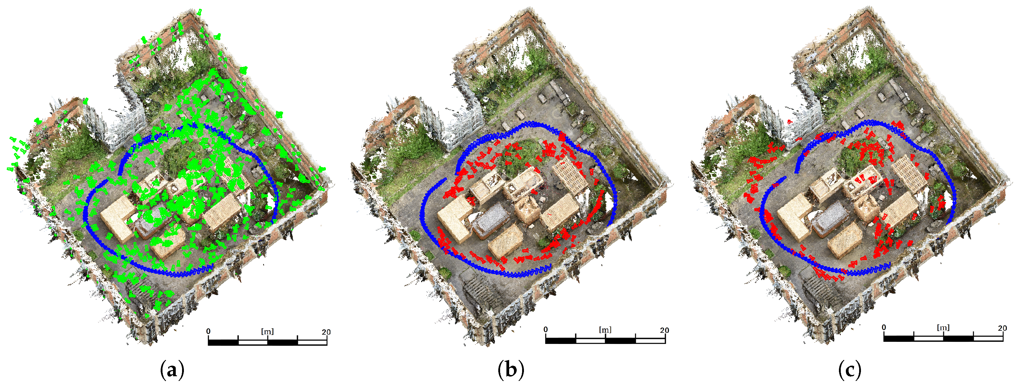
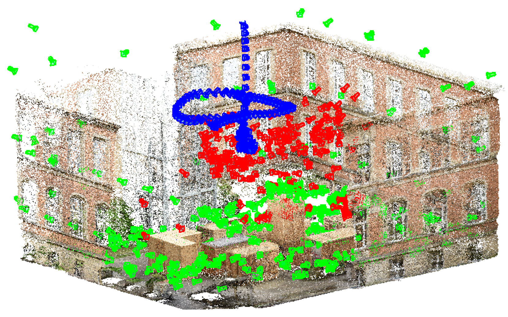
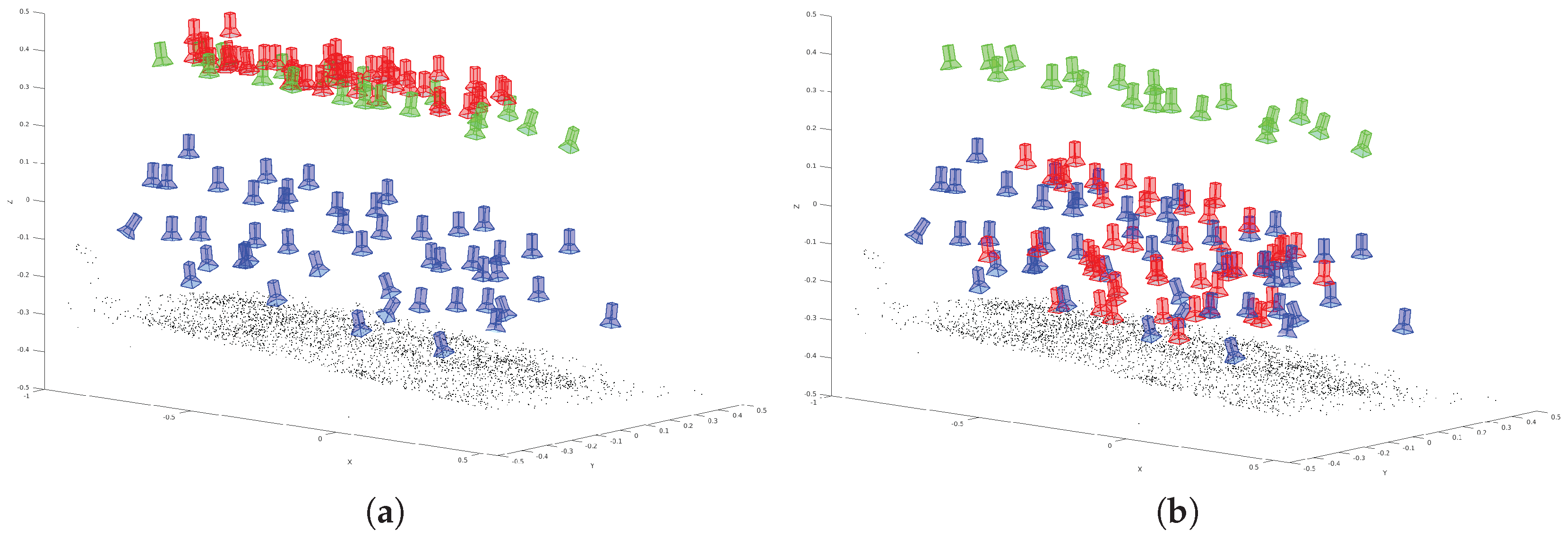
This sequence shows a medium coverage between training and evaluation poses. A high coverage would be given by a more dense distribution of training data or a high similarity of training images and evaluation images. However, Figure 8a shows the training (green) and ground truth (blue) camera poses for the medium coverage sequence. The estimated poses derived by the adaptation of VGG16-Net are visualized (red) in Figure 8b. The poses derived by SqueezePoseNet are visualized in Figure 8c.
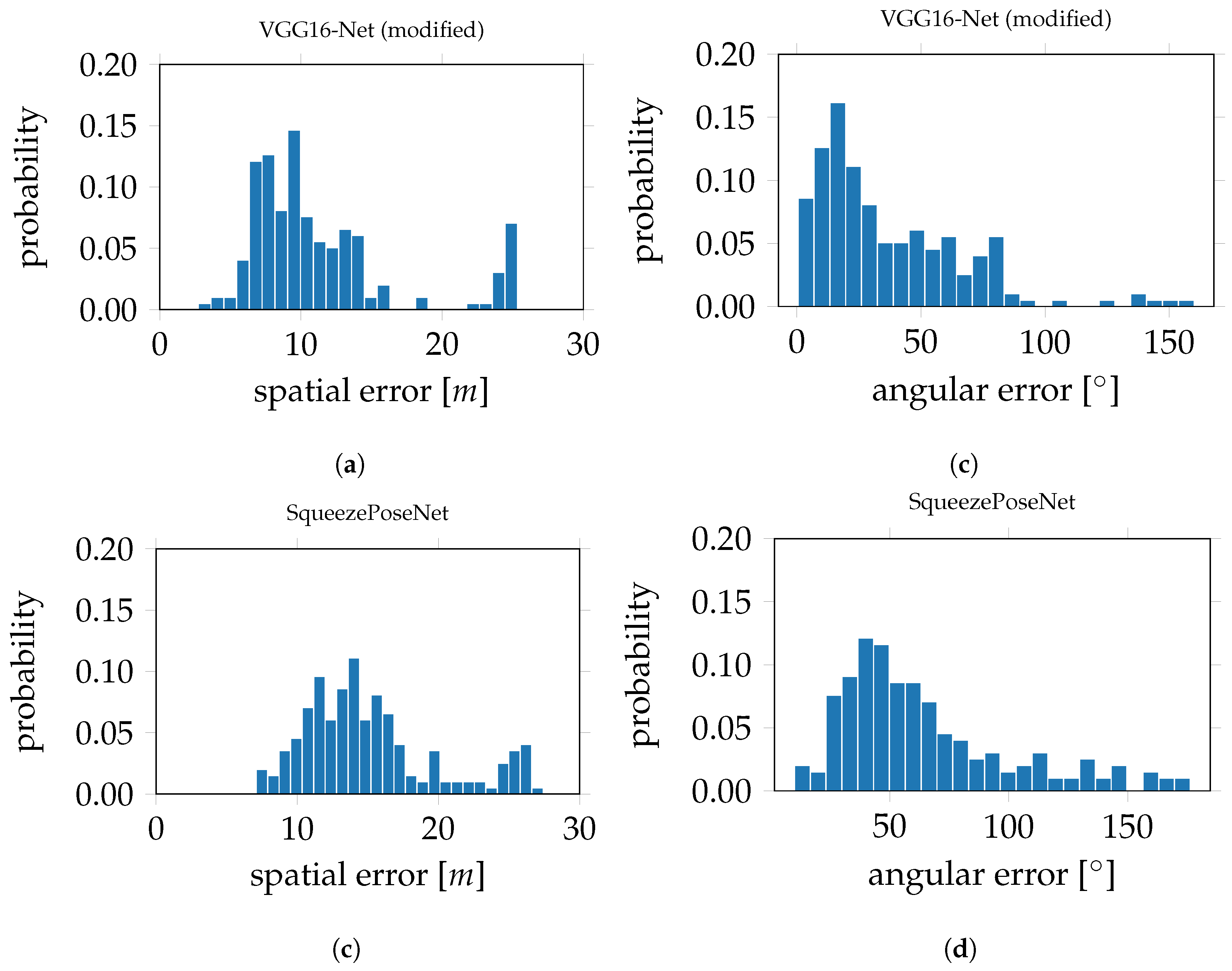
The histograms in Figure 9 show the derived errors to the ground truth poses. Figure 9a,c show the spatial errors of the modified VGG16-Net and SqueezePoseNet to ground truth. Figure 9b,d show the angular errors in the same manner. The evaluation errors are represented by the difference between the spatial and angular estimates to the ground truth. The evaluation errors for the tested CNNs on the Atrium sequences are shown in Table 1 and are as follows. The pose estimation accuracy is 4.91 m and 33.30° for the modified VGG16-Net, 5.19 m and 29.28° for SqueezePoseNet and 8.60 m and 50.83° for PoseNet.
7.2. Low Coverage Sequence
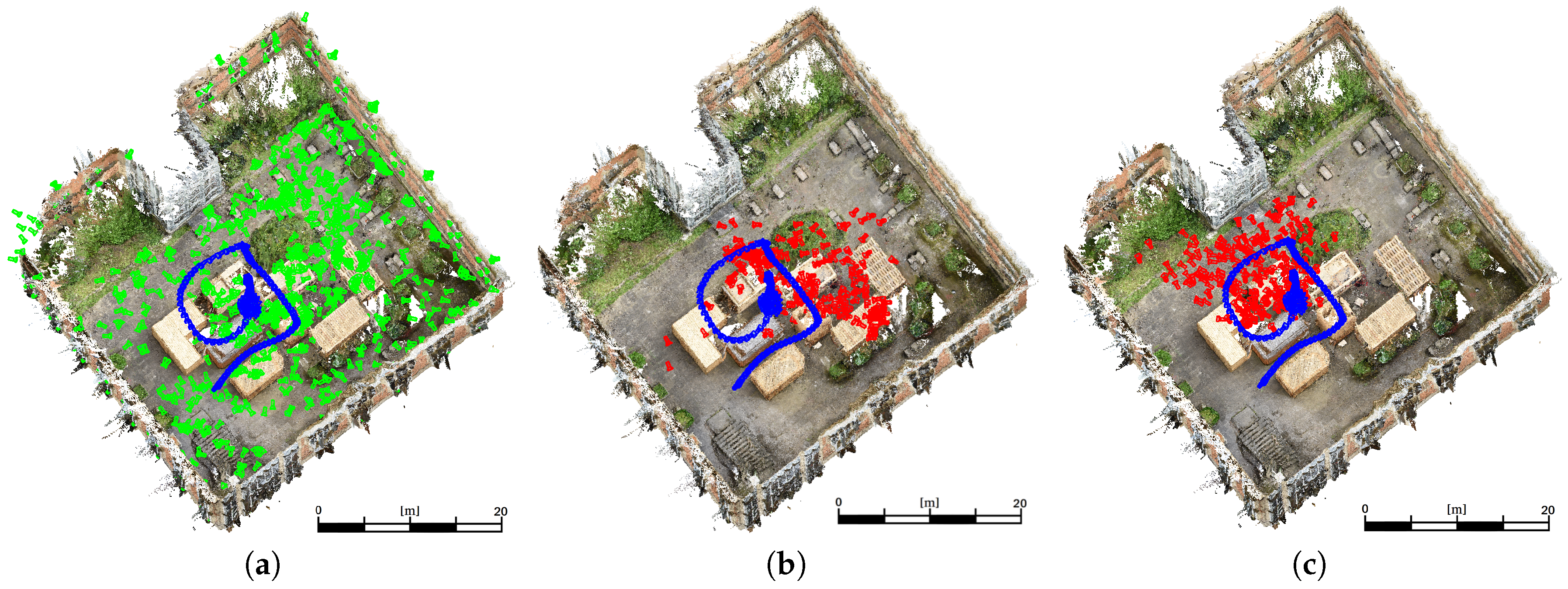
This sequence shows a low coverage between training poses and evaluation poses. Figure 10a shows the training (green) and ground truth (blue) camera poses for the low coverage sequence. The resulting poses derived by the modified VGG16-Net are visualized (red) in Figure 10b. The poses derived by SqueezePoseNet are visualized in Figure 10c. The histograms in Figure 11 show the derived errors to the ground truth poses. Figure 11a,c show the spatial errors of the modified VGG16-Net and SqueezePoseNet, respectively, to ground truth. Figure 11b,d show the angular errors in the same manner. The pose estimation accuracy is 11.34 m and 37.33° for the modified VGG16-Net, 15.18 m and 65.02° for SqueezePoseNet and 11.47 m and 46.40° for PoseNet (Table 1).
An exemplary visualization of a side view is pictured in Figure 12. Green cameras indicate training data, blue cameras depict the ground truth and red cameras are estimated poses derived by the modified VGG16-Net. As can be seen, a major deficit arises in the estimation of the height component; the resulting poses are estimated systematically too low. This behavior is supposed to be influenced by the training poses, which are located far away and mainly on the ground.
7.3. Puzzle Data Set and Data Augmentation
To tackle and overcome the issue of the experienced limited extrapolation capability of CNNs for pose regression (Figure 12), the Puzzle data set was created and augmented with simulated images (Section 5.3). The training data—specifically the lack of training data in the spatial neighborhood of the evaluation data–hardly causes the limitation in extrapolation. Therefore, the net never learned that poses appear in such locations. By adding simulated images of the environment in the spatial neighborhood of the evaluation data, the results would be enhanced. However, such images do not exist in the original Puzzle data set and it is expected that on the application level, such data is not available most of the time. Therefore, the training data set was augmented as described earlier in Section 5.3.
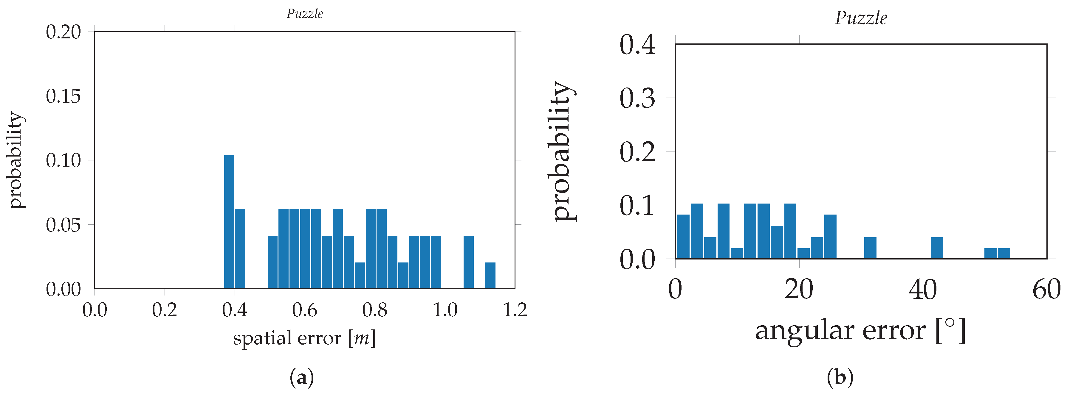
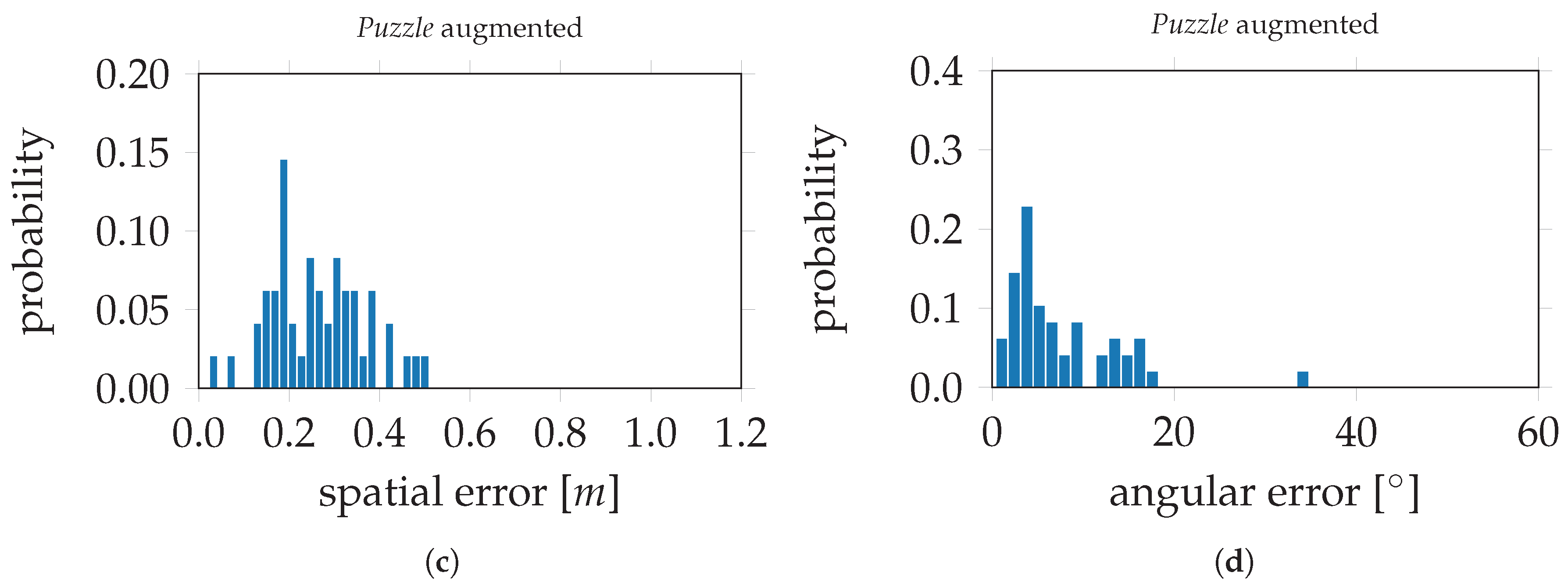
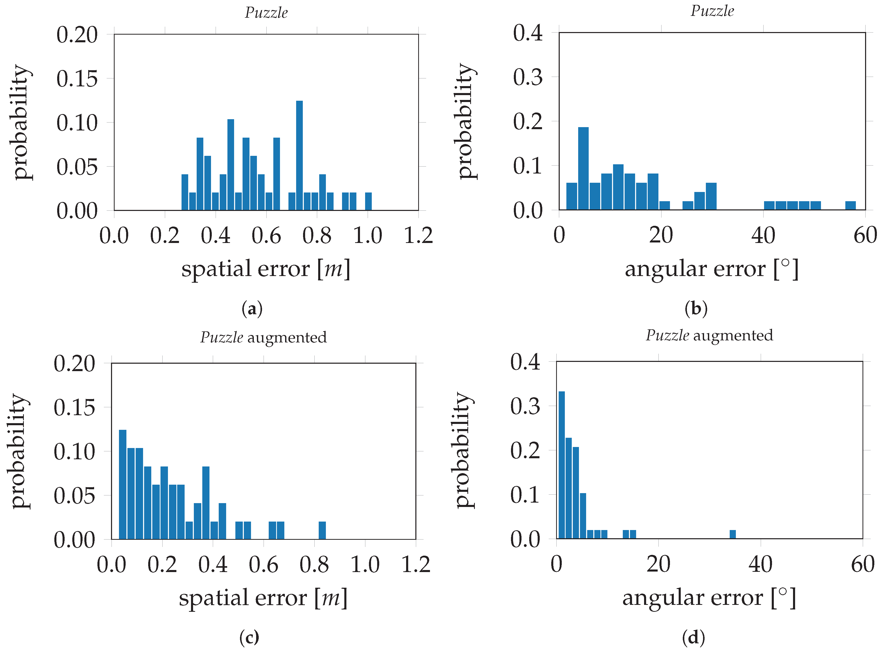
PoseNet and the modified VGG16-Net are trained and evaluated on the Puzzle data set as well as on the Puzzle data set augmented with simulated images. The results on PoseNet are visualized in Figure 13; Figure 13a depicts the results on the original Puzzle data set; Figure 13b shows the results trained on the Puzzle data set after data augmentation. The results on VGG16-Net are visualized in Figure 14; Figure 14a depicts the results on the original Puzzle data set; Figure 14b shows the results trained on the Puzzle data set after data augmentation. The numerical results are shown in Table 2 and are as follows. For PoseNet, trained on the original Puzzle data set, the evaluation errors are 0.47 m and 16.07° for the spatial and angular components, respectively. The evaluation errors on PoseNet, trained on the Puzzle data set after data augmentation, are 0.18 m and 7.53°. This is an improvement of 61.7% for the spatial component and 53.1% for the angular component. In Figure 15, the evaluation errors are visualized in histograms; Figure 15a,b depict the spatial and angular errors, respectively, based on training on the standard Puzzle data set. The histograms in Figure 15c,d depict the spatial and angular errors, respectively, based on training on the Puzzle data set after data augmentation. For the modified VGG16-Net, trained on the original Puzzle data set, the spatial and angular errors are 0.39 m and 17.07° respectively. The evaluation errors on VGG16-Net, trained on the Puzzle data set after data augmentation, are 0.16 m and 4.10°. This is an improvement of 59.0% for the spatial component and 76.0% for the angular component. In Figure 16, the evaluation errors are visualized in histograms; Figure 16a,b depict the spatial and angular errors, respectively, based on training on the standard Puzzle data set. The histograms in Figure 16c,d depict the spatial and angular errors based on training on the Puzzle data set after data augmentation.
8. Discussion
The previous experiments show that Convolutional Neural Networks are capable of estimating camera poses. Even the small SqueezePoseNet could successfully estimate sufficient poses and is very well suited for UAS or MAV on-board applications, due to its small net size.
SqueezePoseNet for CNN-based pose regression is tested on the medium and the low coverage sequence. The medium coverage sequence shows satisfying results for regressing a coarse pose. Pose regression performed well for the VGG16-Net adaptation as well as for SqueezePoseNet. However, VGG16-Net shows more accurate results, as it is deeper than SqueezePoseNet. Both CNNs, with position differences to ground truth of 4.91 m and 5.19 m, respectively, would provide good initial poses for a further and optional pose refinement step. Additionally, the calculation of these poses is processed within a few milliseconds.
As expected, the low coverage sequence where no similar training data was captured showed less accurate results. The spatial differences of 11.34 m and 15.18 m in an environment of about 39 m × 36 m × 18 m are not sufficient. The majority of the position error is influenced by a faulty height determination. The poses are systematically estimated too low. It is to be expected that the CNN cannot extend its knowledge too far from the trained data, as it has never learned such extents. Although interpolation works well, extrapolation performs less well.
To overcome this issue of insufficient coverage, data augmentation was introduced. The Puzzle data set serves to demonstrate the feasibility of this approach. After extending a data set with simulated images, the utilized CNNs perform significantly better in the corresponding environment. On the modified VGG16-Net, the results could be improved by about 59.0% for the position component and 76.0% for the angular component. For PoseNet, the improvement was about 61.7% and 53.1% respectively. It is to be noted that no additional data has to be utilized to achieve that improvement, since the simulated images were rendered from a 3D model, which was generated by the original data set itself.
9. Conclusions and Outlook
It is shown that CNN-based solutions for pose regression can support UAV-based navigation applications and have the potential to improve or substitute existing methods. SqueezeNets architecture could be modified, whereby a small CNN for pose regression, named SqueezePoseNet, could be introduced. The results on this net were promising compared to deeper CNNs, such as PoseNet or VGG16-Net.
A drawback of the proposed idea for UAV navigation is the need for training data. A pose can only be determined if sufficient training data of the environment is available, but such data is often not given. However, image data is captured all over the globe; it is commercially or publicly available. A well known example is the reconstruction of parts of the city of Rome by using solely online data [59]. Additionally, there is a lot of aerial imagery available covering urban and rural areas, which may also serve as training data.
Furthermore, the issue of lacking training data was tackled by extending a training set with simulated images by data augmentation. Thereby, the evaluation errors could be decreased by 59.0–61.7% for position and 53.1–76.0% for rotation, compared to the corresponding not-augmented data set. This indicates the success of supporting Convolutional Neural Networks with simulated images to learn extrapolation for pose regression. For this data augmentation, a 3D model of the environment is mandatory. Data for such models could be obtained by accessing the aforementioned image data bases. The reconstruction of 3D models is a basis for rendering images of a target environment. In this contribution, a photo-realistic model was created to render additional images. It is of further interest whether simple triangulated 3D models may serve for data augmentation on pose regression with similar success. By utilizing such 3D models, a CNN-based or -aided navigation approach could be realized.
Of further interest is the amount of data content which can be learned by a CNN, especially by a small CNN. Even though the number of weighting parameters of the CNNs do not increase with a higher amount of training images, a CNN is only able to recognize a finite part of the training data. Different sized CNNs such as PoseNet, VGG16-Net or SqueezePoseNet may fail or at least might have different accuracies depending on the given size of the net itself or the training environment. Both should be investigated to determine the optimal performance for given applications. Furthermore, the investigation of data augmentation with more and diversified simulated images and on larger data sets with real-world examples will be tackled in future work.
Author Contributions
Markus S. Mueller and Boris Jutzi contributed to design the study, develop the methodology, collect the data, perform the analysis, and wrote the manuscript.
Conflicts of Interest
The authors declare no conflict of interest.
References
- Li-Chee-Ming, J.; Armenakis, C. Augmenting ViSP’s 3D Model-Based Tracker with RGB-D SLAM for 3D Pose Estimation in Indoor Environments. Int. Arch. Photogramm. Remote Sens. Spat. Inf. Sci. 2016, 41, 925–932. [Google Scholar] [CrossRef]
- Engel, J.; Koltun, V.; Cremers, D. Direct sparse odometry. arXiv, 2016; arXiv:1607.02565. [Google Scholar]
- Engel, J.; Schöps, T.; Cremers, D. LSD-SLAM: Large-Scale Direct Monocular SLAM. In Proceedings of the European Conference on Computer Vision, Zurich, Switzerland, 6–12 September 2014; pp. 834–849. [Google Scholar]
- Mur-Artal, R.; Montiel, J.M.M.; Tardós, J.D. ORB-SLAM: A Versatile and Accurate Monocular SLAM System. IEEE Trans. Robot. 2015, 31, 1147–1163. [Google Scholar] [CrossRef]
- Nvidia. 2017. Available online: http://www.nvidia.com/docs/IO/90715/Tegra_Multiprocessor_Architecture_white_paper_Final_v1.1.pdf (accessed on 12 December 2017).
- Kendall, A.; Grimes, M.; Cipolla, R. Posenet: A convolutional network for real-time 6-dof camera relocalization. In Proceedings of the IEEE International Conference on Computer Vision, Santiago, Chile, 7–13 December 2015; pp. 2938–2946. [Google Scholar]
- Lowe, D.G. Object recognition from local scale-invariant features. In Proceedings of the Seventh IEEE International Conference on Computer Vision, Kerkyra, Greece, 20–27 September 1999; Volume 2, pp. 1150–1157. [Google Scholar]
- Rublee, E.; Rabaud, V.; Konolige, K.; Bradski, G. ORB: An efficient alternative to SIFT or SURF. In Proceedings of the 2011 International Conference on Computer Vision, Barcelona, Spain, 6–13 November 2011; pp. 2564–2571. [Google Scholar]
- Bay, H.; Tuytelaars, T.; van Gool, L. Surf: Speeded up robust features. In Proceedings of the European Conference on Computer Vision, Graz, Austria, 7–13 May 2006; pp. 404–417. [Google Scholar]
- Mueller, M.S.; Urban, S.; Jutzi, B. SqueezePoseNet: Image based Pose Regression with small Convolutional Neural Networks for Real Time UAS Navigation. ISPRS Ann. Photogramm. Remote Sens. Spat. Inf. Sci. 2017, 4, 49–57. [Google Scholar] [CrossRef]
- Conte, G.; Doherty, P. Vision-based Unmanned Aerial Vehicle Navigation Using Geo-referenced Information. EURASIP J. Adv. Signal Process. 2009. [Google Scholar] [CrossRef]
- Conte, G.; Doherty, P. A visual navigation system for uas based on geo-referenced imagery. Int. Arch. Photogramm. Remote Sens. Spat. Inf. Sci. 2011, 38, 1. [Google Scholar] [CrossRef]
- Li, Q.; Wang, G.; Liu, J.; Chen, J. Robust scale-invariant feature matching for remote sensing image registration. IEEE Geosci. Remote Sens. Lett. 2009, 6, 287–291. [Google Scholar]
- Ma, J.; Zhou, H.; Zhao, J.; Gao, Y.; Jiang, J.; Tian, J. Robust Feature Matching for Remote Sensing Image Registration via Locally Linear Transforming. IEEE Trans. Geosci. Remote Sens. 2015, 53, 6469–6481. [Google Scholar] [CrossRef]
- Yang, H.; Zhang, S.; Wang, Y. Robust and precise registration of oblique images based on scale-invariant feature transformation algorithm. IEEE Geosci. Remote Sens. Lett. 2012, 9, 783–787. [Google Scholar] [CrossRef]
- Ma, J.; Zhao, J.; Guo, H.; Jiang, J.; Zhou, H.; Gao, Y. Locality Preserving Matching. In Proceedings of the International Joint Conference on Artificial Intelligence, Melbourne, Australia, 19–25 August 2017; pp. 4492–4498. [Google Scholar]
- Reitmayr, G.; Drummond, T. Going out: Robust model-based tracking for outdoor augmented reality. In Proceedings of the 5th IEEE and ACM International Symposium on Mixed and Augmented Reality, Santa Barbard, CA, USA, 22–25 October 2006; pp. 109–118. [Google Scholar]
- Unger, J.; Rottensteiner, F.; Heipke, C. Integration of a generalised building model into the pose estimation of uas images. Int. Arch. Photogramm. Remote Sens. Spat. Inf. Sci. 2016, 41, 1057–1064. [Google Scholar] [CrossRef]
- Mueller, M.S.; Voegtle, T. Determination of steering wheel angles during car alignment by image analysis methods. Int. Arch. Photogramm. Remote Sens. Spat. Inf. Sci. 2016, 41, 77–83. [Google Scholar] [CrossRef]
- Ulrich, M.; Wiedemann, C.; Steger, C. CAD-based recognition of 3D objects in monocular images. In Proceedings of the International Conference on Robotics and Automation, Kobe, Japan, 12–17 May 2009; Volume 9, pp. 1191–1198. [Google Scholar]
- Urban, S.; Leitloff, J.; Wursthorn, S.; Hinz, S. Self-Localization of a Multi-Fisheye Camera Based Augmented Reality System in Textureless 3D Building Models. ISPRS Ann. Photogramm. Remote Sens. Spat. Inf. Sci. 2013, 43–48. [Google Scholar] [CrossRef]
- Zang, C.; Hashimoto, K. Camera localization by CAD model matching. In Proceedings of the 2011 IEEE/SICE International Symposium on System Integration, Kyoto, Japan, 20–22 December 2011; pp. 30–35. [Google Scholar]
- Altwaijry, H.; Trulls, E.; Hays, J.; Fua, P.; Belongie, S. Learning to match aerial images with deep attentive architectures. In Proceedings of the IEEE Conference on Computer Vision and Pattern Recognition, Las Vegas, NV, USA, 27–30 June 2016; pp. 3539–3547. [Google Scholar]
- Lin, T.-Y.; Cui, Y.; Belongie, S.; Hays, J. Learning deep representations for ground-to-aerial geolocalization. In Proceedings of the IEEE Conference on Computer Vision and Pattern Recognition, Boston, MA, USA, 7–12 June 2015; pp. 5007–5015. [Google Scholar]
- Kendall, A.; Cipolla, R. Modelling uncertainty in deep learning for camera relocalization. In Proceedings of the International Conference on Robotics and Automation, Stockholm, Sweden, 16–21 May 2016; pp. 4762–4769. [Google Scholar]
- Szegedy, C.; Liu, W.; Jia, Y.; Sermanet, P.; Reed, S.; Anguelov, D.; Erhan, D.; Vanhoucke, V.; Rabinovich, A. Going deeper with convolutions. In Proceedings of the IEEE Conference on Computer Vision and Pattern Recognition, Boston, MA, USA, 7–12 June 2015; pp. 1–9. [Google Scholar]
- Walch, F.; Hazirbas, C.; Leal-Taixé, L.; Sattler, T.; Hilsenbeck, S.; Cremers, D. Image-based Localization with Spatial LSTMs. arXiv, 2016; arXiv:1611.07890. [Google Scholar]
- Hochreiter, S.; Schmidhuber, J. Long short-term memory. Neural Comput. 1997, 9, 1735–1780. [Google Scholar] [CrossRef] [PubMed]
- Li, R.; Liu, Q.; Gui, J.; Gu, D.; Hu, H. Indoor relocalization in challenging environments with dual-stream convolutional neural networks. IEEE Trans. Autom. Sci. Eng. 2017, PP, 1–12. [Google Scholar] [CrossRef]
- Simonyan, K.; Zisserman, A. Very deep convolutional networks for large-scale image recognition. arXiv, 2014; arXiv:1409.1556. [Google Scholar]
- Iandola, F.N.; Han, S.; Moskewicz, M.W.; Ashraf, K.; Dally, W.J.; Keutzer, K. SqueezeNet: AlexNet-level accuracy with 50× fewer parameters and <0.5 mb model size. arXiv, 2016; arXiv:1602.07360. [Google Scholar]
- Wu, J.; Leng, C.; Wang, Y.; Hu, Q.; Cheng, J. Quantized convolutional neural networks for mobile devices. In Proceedings of the IEEE Conference on Computer Vision and Pattern Recognition, Caesars Palace, NV, USA, 26 June–1 July 2016; pp. 4820–4828. [Google Scholar]
- Courbariaux, M.; Hubara, I.; Soudry, D.; El-Yaniv, R.; Bengio, Y. Binarized neural networks: Training deep neural networks with weights and activations constrained to + 1 or −1. arXiv, 2016; arXiv:1602.02830. [Google Scholar]
- Dosovitskiy, A.; Fischer, P.; Springenberg, J.T.; Riedmiller, M.; Brox, T. Discriminative unsupervised feature learning with exemplar convolutional neural networks. IEEE Trans. Pattern Anal. Mach. Intell. 2016, 38, 1734–1747. [Google Scholar] [CrossRef] [PubMed]
- Gharbi, M.; Chaurasia, G.; Paris, S.; Durand, F. Deep Joint Demosaicking and Denoising. ACM Trans. Graph. (TOG) 2016, 35, 191. [Google Scholar] [CrossRef]
- Lemley, J.; Bazrafkan, S.; Corcoran, P. Smart Augmentation—Learning an Optimal Data Augmentation Strategy. IEEE Access 2017, 5, 5858–5869. [Google Scholar] [CrossRef]
- Paulin, M.; Revaud, J.; Harchaoui, Z.; Perronnin, F.; Schmid, C. Transformation pursuit for image classification. In Proceedings of the IEEE Conference on Computer Vision and Pattern Recognition, Columbus, OH, USA, 23–28 June 2014; pp. 3646–3653. [Google Scholar]
- Cui, X.; Goel, V.; Kingsbury, B. Data augmentation for deep neural network acoustic modeling. IEEE/ACM Trans. Audio Speech Lang. Process. (TASLP) 2015, 23, 1469–1477. [Google Scholar]
- Vedaldi, O.M.P.A.; Zisserman, A. Deep Face Recognition. In Proceedings of the British Machine Vision Conference, Swansea, UK, 7–10 September 2015; Volume 1, p. 6. [Google Scholar]
- Michels, J.; Saxena, A.; Ng, A.Y. High Speed Obstacle Avoidance Using Monocular Vision and Reinforcement Learning. In Proceedings of the 22nd International Conference on Machine Learning, Bonn, Germany, 7–11 August 2005; ACM: New York, NY, USA, 2005. [Google Scholar]
- Stark, M.; Goesele, M.; Schiele, B. Back to the Future: Learning Shape Models from 3D CAD Data. In Proceedings of the British Machine Vision Conference, Aberystwyth, UK, 31 August–3 September 2010; Volume 2, pp. 106.1–106.11. [Google Scholar]
- Gupta, S.; Arbeláez, P.; Girshick, R.; Malik, J. Inferring 3D Object Pose in RGB-D Images. arXiv, 2015; arXiv:1502.04652. [Google Scholar]
- Su, H.; Qi, C.R.; Li, Y.; Guibas, L.J. Render for CNN: Viewpoint estimation in images using CNNs trained with rendered 3D model views. In Proceedings of the IEEE International Conference on Computer Vision, Santiago, Chile, 7–13 December 2015; pp. 2686–2694. [Google Scholar]
- Ivarsson, C. Combining Street View and Aerial Images to Create Photo-Realistic 3D City Models. Master’s Thesis, Royal Institute of Technology, Stockholm, Sweden, 2014. [Google Scholar]
- Poullis, C.; You, S. Photorealistic Large-Scale Urban City Model Reconstruction. IEEE Trans. Vis. Comput. Graph. 2009, 15, 654–669. [Google Scholar] [CrossRef] [PubMed]
- Se, S.; Jasiobedzki, P. Photo-Realistic 3D Model Reconstruction. In Proceedings of the 2006 IEEE International Conference on Robotics and Automation, Orlando, FL, USA, 15–19 May 2006; pp. 3076–3082. [Google Scholar]
- Pollefeys, M.; Koch, R.; Vergauwen, M.; van Gool, L. Automated Reconstruction of 3D Scenes from Sequences of Images. ISPRS J. Photogramm. Remote Sens. 2000, 55, 251–267. [Google Scholar] [CrossRef]
- Singh, S.P.; Jain, K.; Mandla, V.R. Virtual 3D City Modeling: Techniques and Applications. Int. Arch. Photogramm. Remote Sens. Spat. Inf. Sci. 2013. [Google Scholar] [CrossRef]
- Sattler, T.; Maddern, W.; Torii, A.; Sivic, J.; Pajdla, T.; Pollefeys, M.; Okutomi, M. Benchmarking 6DOF Urban Visual Localization in Changing Conditions. arXiv, 2017; arXiv:1707.09092. [Google Scholar]
- Maas, A.L.; Hannun, A.Y.; Ng, A.Y. Rectifier nonlinearities improve neural network acoustic models. In Proceedings of the International Conference on Machine Learning, Atlanta, GA, USA, 16–21 June 2013; Volume 30. [Google Scholar]
- Ioffe, S.; Szegedy, C. Batch normalization: Accelerating deep network training by reducing internal covariate shift. In Proceedings of the 32nd International Conference on Machine Learning, Lille, France, 6–11 July 2015; pp. 448–456. [Google Scholar]
- PhotoModeler; Corporate Head Office, Eos Systems Inc.: Vancouver, BC, Canada, 2017.
- Koenig, N.; Howard, A. Design and use paradigms for gazebo, an open-source multi-robot simulator. In Proceedings of the IEEE/RSJ International Conference on Intelligent Robots and Systems, Sendai, Japan, 28 September–2 October 2004; Volume 3. [Google Scholar]
- Krizhevsky, A.; Sutskever, I.; Hinton, G.E. Imagenet classification with deep Convolutional Neural Networks. In Proceedings of the 25th International Conference on Neural Information Processing Systems, Lake Tahoe, NV, USA, 3–6 December 2012; pp. 1097–1105. [Google Scholar]
- Zhou, B.; Khosla, A.; Lapedriza, A.; Torralba, A.; Oliva, A. Places: An image database for deep scene understanding. arXiv, 2016; arXiv:1610.02055. [Google Scholar]
- Zhou, B.; Lapedriza, A.; Xiao, J.; Torralba, A.; Oliva, A. Learning deep features for scene recognition using places database. Adv. Neural Inf. Process. Syst. 2014, 487–495. [Google Scholar]
- Urban, S.; Jutzi, B. LaFiDa—A Laserscanner Multi-Fisheye Camera Dataset. J. Imaging 2017, 3, 5. [Google Scholar] [CrossRef]
- Agisoft. Agisoft LLC. 2017. Available online: http://www.agisoft.com/ (accessed on 12 December 2017).
- Agarwal, S.; Furukawa, Y.; Snavely, N.; Simon, I.; Curless, B.; Seitz, S.M.; Szeliski, R. Building rome in a day. Commun. ACM 2011, 54, 105–112. [Google Scholar] [CrossRef]
Figure 1.
Architecture of SqueezePoseNet. A fully connected layer with 500 neurons is added after the last pooling layer. For pose estimation, two fully connected layers (Position and Rotation) with 3 and 4 neurons, respectively, were added.
Figure 1.
Architecture of SqueezePoseNet. A fully connected layer with 500 neurons is added after the last pooling layer. For pose estimation, two fully connected layers (Position and Rotation) with 3 and 4 neurons, respectively, were added.
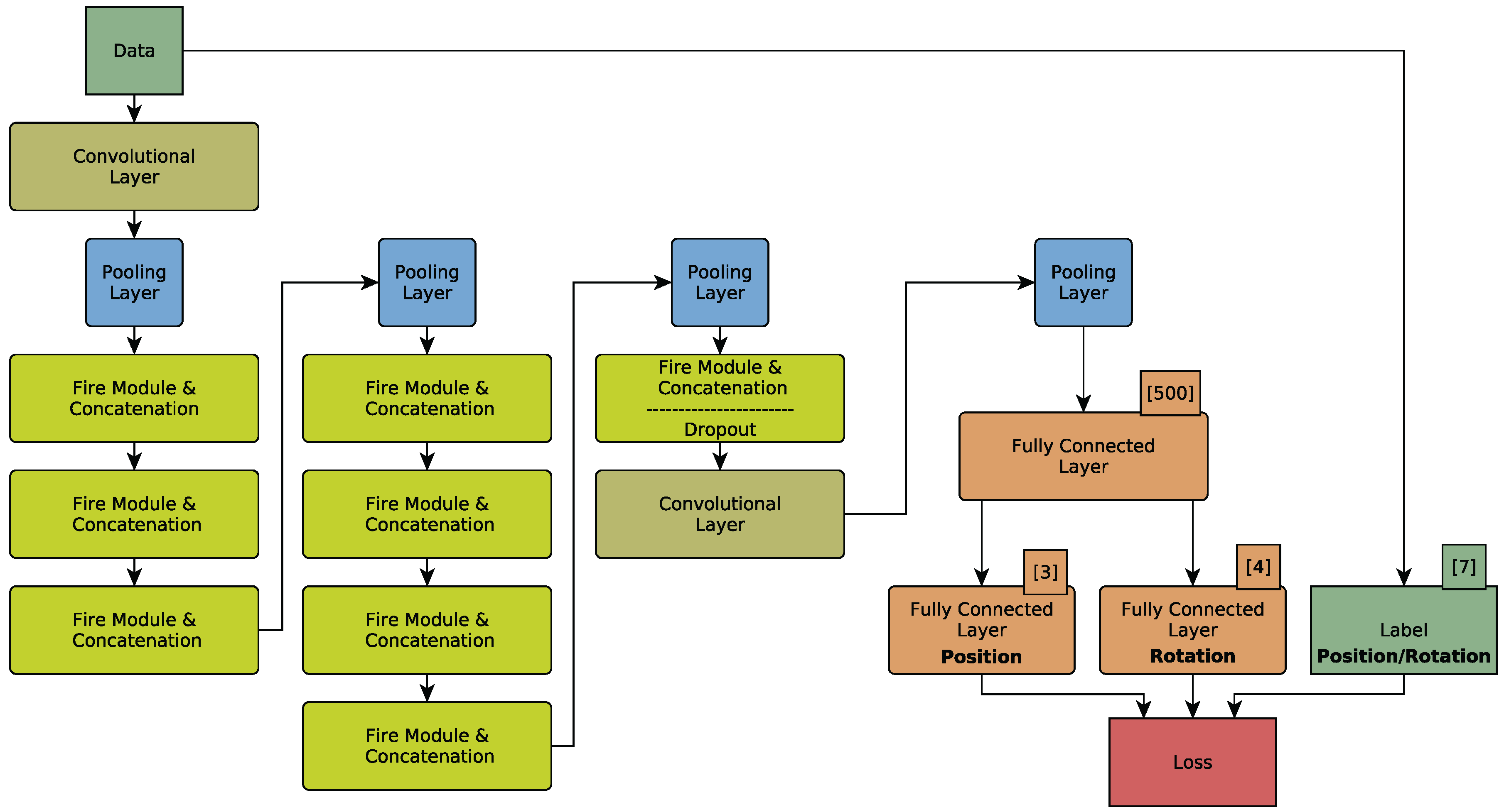
Figure 2.
Architecture of a Fire module. A so-called squeeze operation [31] is performed by the 1 × 1 convolutional layer. Subsequently, an expand operation that is a combination of 1 × 1 and 3 × 3 filters increases the number of activation maps while keeping the number of parameters low.
Figure 2.
Architecture of a Fire module. A so-called squeeze operation [31] is performed by the 1 × 1 convolutional layer. Subsequently, an expand operation that is a combination of 1 × 1 and 3 × 3 filters increases the number of activation maps while keeping the number of parameters low.
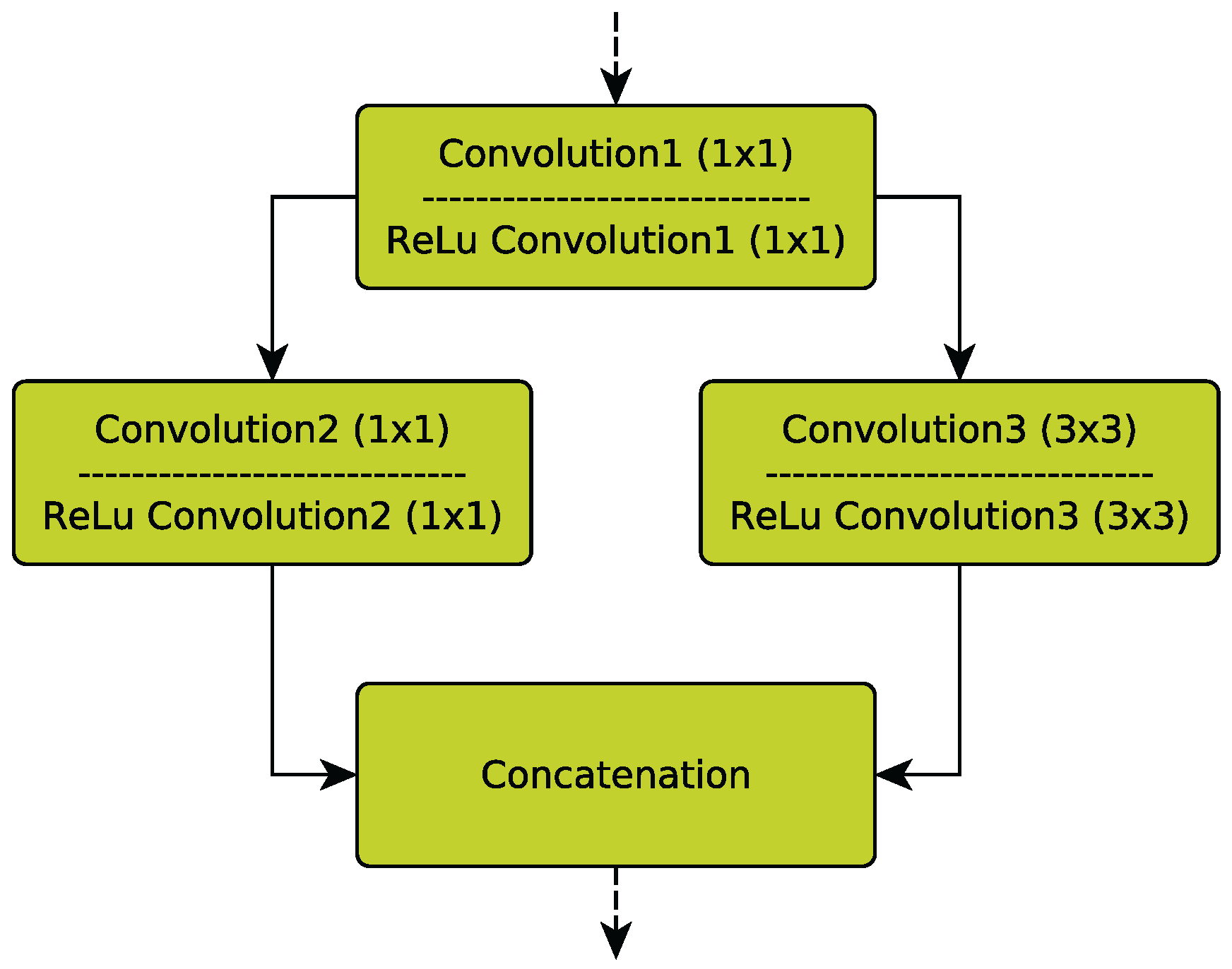
Figure 3.
Side views of the Atrium. To obtain a complete introduction to the environment, the 3D model of the Atrium is visualized in east view (a) and west view (b). Notice, the red-bricked walls show very similar structures, forming a challenging environment for computer vision algorithms.
Figure 3.
Side views of the Atrium. To obtain a complete introduction to the environment, the 3D model of the Atrium is visualized in east view (a) and west view (b). Notice, the red-bricked walls show very similar structures, forming a challenging environment for computer vision algorithms.
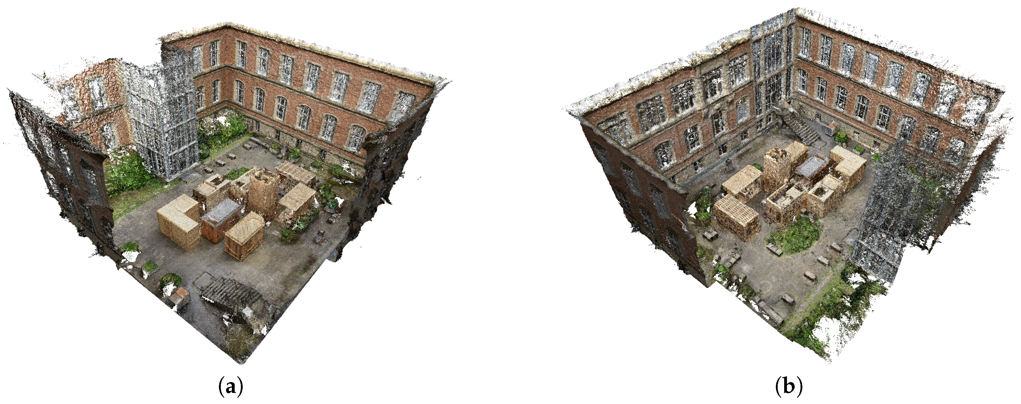
Figure 4.
Example images of the Atrium. (a) Windows in the scene cause reflections; this is challenging for computer vision tasks; (b) Image captured with high (angular) motion thus showing motion blur; (c) Image shows ambiguous structures; (d) Test image of the low coverage sequence (Section 7.2) captured at high altitude. A similar perspective is not contained in the training data; the pose is ‘far away’ from any training pose (position as well as orientation).

Figure 5.
Nadir view of the puzzle’s 3D model. This model was generated with 19 images and serves to render additional images for data augmentation on the Puzzle data set.
Figure 5.
Nadir view of the puzzle’s 3D model. This model was generated with 19 images and serves to render additional images for data augmentation on the Puzzle data set.
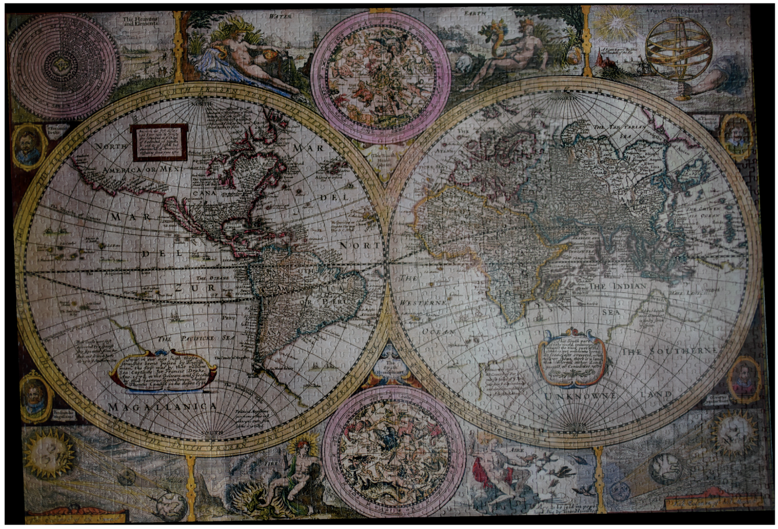
Figure 6.
The top row shows images taken for the Puzzle data set; the bottom row shows corresponding simulated images from a photo-realistic model. The pose of the original image (a) is determined incorrectly within the SfM process leading to a faulty simulated image (c). Images with wrong pose determinations were disregarded in all further processes. The pose of image (b) is determined correctly, whereby the simulated image (d) is rendered accordingly.

Figure 7.
DJI Matrice 100 with an on-board processing unit DJI Manifold and a Zenmuse X3 camera.
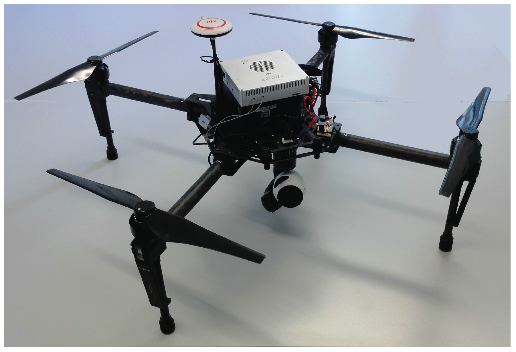
Figure 8.
Atrium data set, medium coverage sequence. (a) Visualization of ground truth; (b) Results derived by the modified VGG16-Net; (c) Results derived by SqueezePoseNet. Green cameras indicate training data, blue cameras depict the ground truth and red cameras are estimated poses derived by the modified CNNs.

Figure 9.
Medium coverage sequence. The histograms show the spatial and angular errors of the CNN-derived poses to ground truth. Histograms (a,c) depict the spatial errors of the modified VGG16-Net and SqueezePoseNet, respectively, and (b,d) show the angular errors.
Figure 9.
Medium coverage sequence. The histograms show the spatial and angular errors of the CNN-derived poses to ground truth. Histograms (a,c) depict the spatial errors of the modified VGG16-Net and SqueezePoseNet, respectively, and (b,d) show the angular errors.
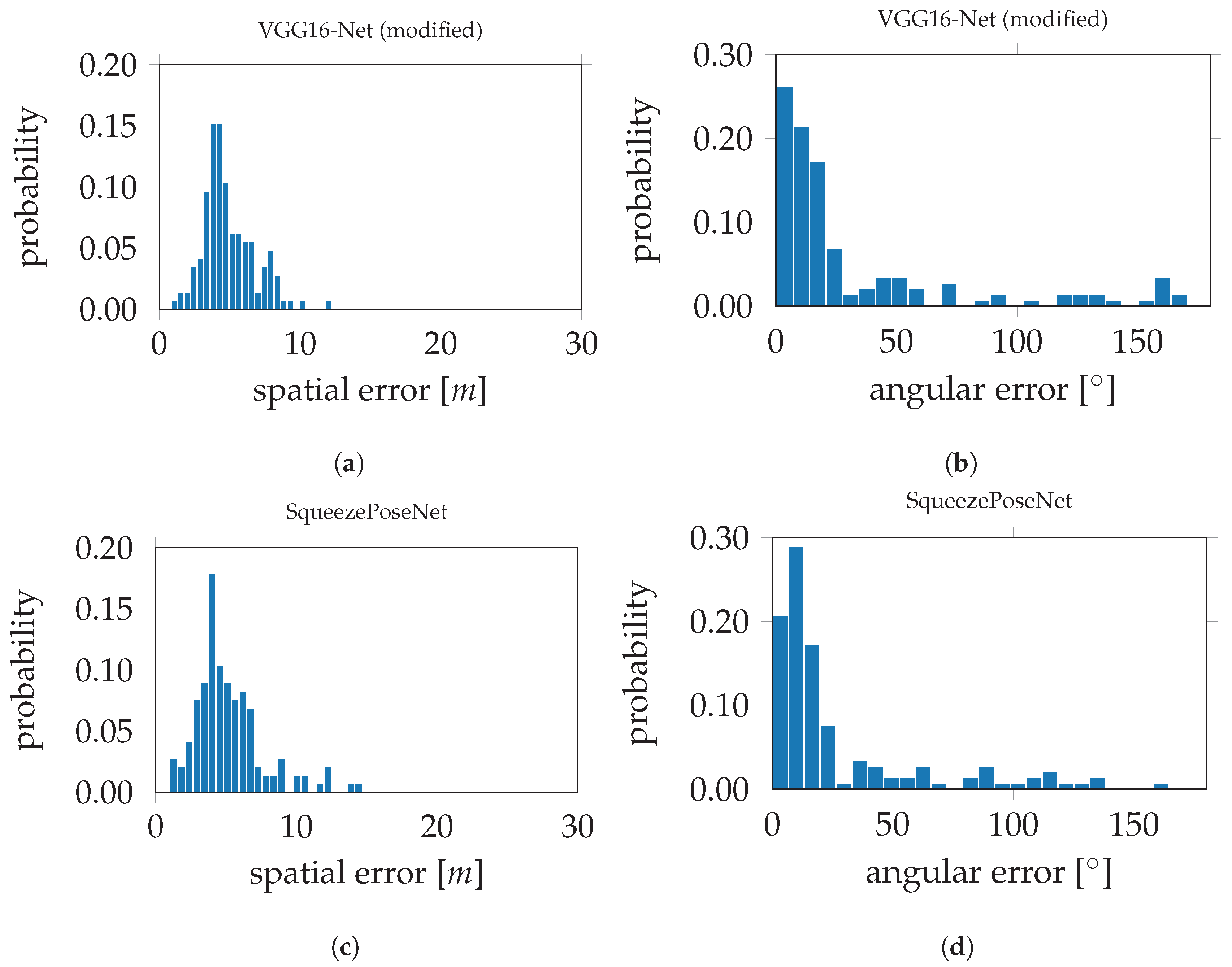
Figure 10.
Atrium data set, low coverage sequence. (a) Visualization of ground truth; (b) Results derived by the modified VGG16-Net; (c) Results derived by SqueezePoseNet. Green cameras indicate training data, blue cameras depict the ground truth and red cameras are estimated poses derived by the modified CNNs.

Figure 11.
Low coverage sequence. The histograms show the spatial and angular errors of the CNN-derived poses to ground truth. Histograms (a,c) depict the spatial errors of the modified VGG16-Net and SqueezePoseNet, respectively, and (b,d) the angular errors.
Figure 11.
Low coverage sequence. The histograms show the spatial and angular errors of the CNN-derived poses to ground truth. Histograms (a,c) depict the spatial errors of the modified VGG16-Net and SqueezePoseNet, respectively, and (b,d) the angular errors.

Figure 12.
Visualization of VGG16-Net results on the Atrium data set. Green cameras indicate training data, blue cameras depict the ground truth and red cameras are estimated poses derived by the modified VGG16-Net. The poses are systematically estimated too low. This behavior is supposed to be influenced by the training poses, which are located far away and mainly on the ground.

Figure 13.
Visualization of determined poses by PoseNet on the Puzzle data set. (a) Pose results for PoseNet trained on the original Puzzle data set; (b) Pose results for PoseNet trained on the Puzzle data set after data augmentation. Green cameras indicate training data of the original Puzzle data set, blue cameras depict the ground truth and red cameras are estimated poses derived by PoseNet. The black points indicate the puzzle’s pointcloud. It is clearly shown that data augmentation supports the extrapolation potential of the net.

Figure 14.
Visualization of determined poses by the modified VGG16-Net on the Puzzle data set. (a) Pose results for the modified VGG16-Net trained on the original Puzzle data set; (b) Pose results for the modified VGG16-Net trained on the Puzzle data set after data augmentation. Green cameras indicate training data of the original Puzzle data set, blue cameras depict the ground truth and red cameras are estimated poses derived by the modified VGG16-Net. The black points indicate the puzzle’s pointcloud. It is clearly shown that data augmentation supports the extrapolation potential of the net.
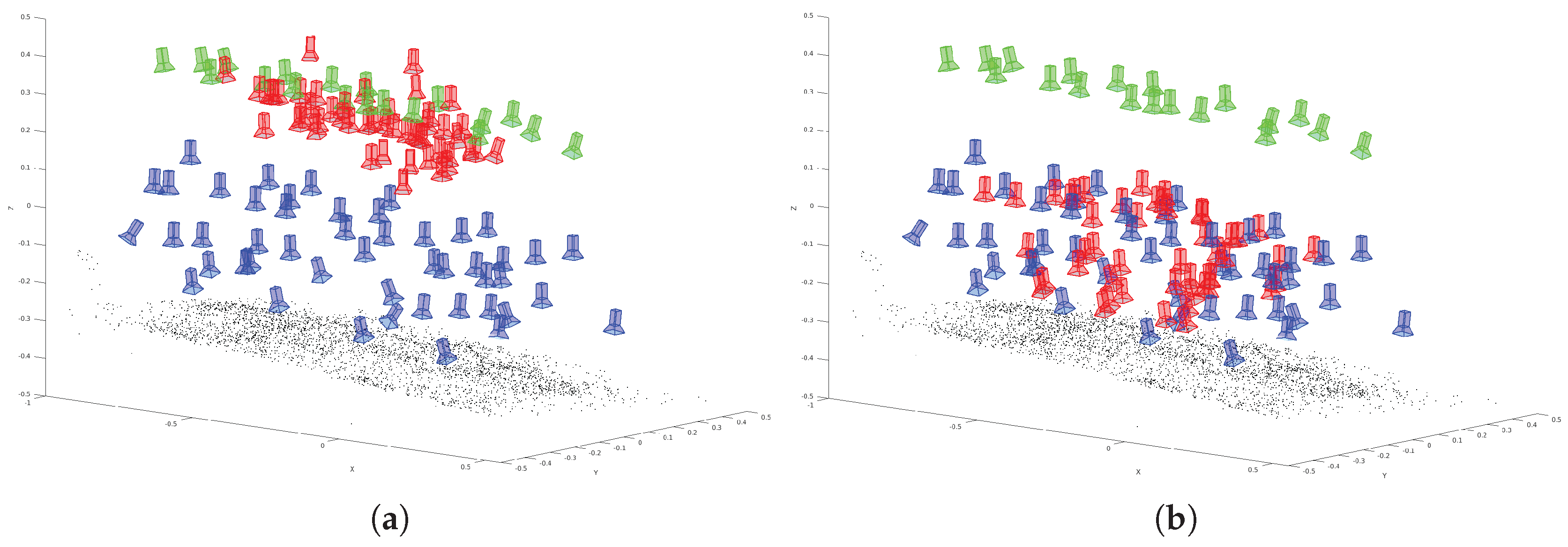
Figure 15.
The histograms show the spatial and angular pose errors derived by PoseNet. Histograms (a,b) depict the spatial and angular errors, respectively, based on training on the standard Puzzle data set; Histograms (c,d) depict the spatial and angular errors, respectively, based on training on the Puzzle extended with simulated images. The mean errors could be decreased from 0.47 m and 16.07° to 0.18 m and 7.53° by data augmentation.


Figure 16.
The histograms show the spatial and angular pose errors derived by VGG16-Net. Histograms (a,b) depict the spatial and angular errors based on training on the standard Puzzle data set; Histograms (c,d) depict the spatial and angular errors based on training on the Puzzle data set extended with simulated images. The mean errors could be decreased from 0.39 m and 17.07° to 0.16 m and 4.10° by data augmentation.


Table 1.
Position and rotation errors on the medium and high coverage sequences, respectively. Bold text marks the best result on a sequence.
Table 1.
Position and rotation errors on the medium and high coverage sequences, respectively. Bold text marks the best result on a sequence.
| Evalutaion Errors (Mean) | PoseNet | VGG16-Net (Modified) | SqueezePoseNet |
|---|---|---|---|
| Medium coverage sequence | 8.60 m, 50.83° | 4.91 m, 33.30° | 5.19 m, 29.28° |
| Low coverage sequence | 11.47 m, 46.40° | 11.34 m, 37.33° | 15.18 m, 65.02° |
Table 2.
Mean evaluation errors for PoseNet and the modified VGG16-Net trained on the original Puzzle data set and the Puzzle data set after data augmentation. The last row shows the percent improvement of training on the augmented data set against the original.
Table 2.
Mean evaluation errors for PoseNet and the modified VGG16-Net trained on the original Puzzle data set and the Puzzle data set after data augmentation. The last row shows the percent improvement of training on the augmented data set against the original.
| Evalutaion Errors (Mean) | Puzzle | Puzzle (Augmented) | Improvement |
|---|---|---|---|
| PoseNet | 0.47 m, 16.07° | 0.18 m, 7.53° | 61.7%, 53.1% |
| modified VGG16-Net | 0.39 m, 17.07° | 0.16 m, 4.10° | 59.0%, 76.0% |
© 2018 by the authors. Licensee MDPI, Basel, Switzerland. This article is an open access article distributed under the terms and conditions of the Creative Commons Attribution (CC BY) license (http://creativecommons.org/licenses/by/4.0/).
Share and Cite
MDPI and ACS Style
Mueller, M.S.; Jutzi, B. UAS Navigation with SqueezePoseNet—Accuracy Boosting for Pose Regression by Data Augmentation. Drones 2018, 2, 7. https://doi.org/10.3390/drones2010007
AMA Style
Mueller MS, Jutzi B. UAS Navigation with SqueezePoseNet—Accuracy Boosting for Pose Regression by Data Augmentation. Drones. 2018; 2(1):7. https://doi.org/10.3390/drones2010007
Chicago/Turabian StyleMueller, Markus S., and Boris Jutzi. 2018. "UAS Navigation with SqueezePoseNet—Accuracy Boosting for Pose Regression by Data Augmentation" Drones 2, no. 1: 7. https://doi.org/10.3390/drones2010007