CFD for Surfboards: Comparison between Three Different Designs in Static and Maneuvering Conditions †

1
NTNU—Norwegian University of Science and Technology—SIAT (Senter for Idrettsanlegg og Teknologi), K. Hejes vei 2b, 7042 Trondheim, Norway
2
Intitutt for Energiteknikk, Instituttveien 18a, 2007 Kjeller, Norway
*
Author to whom correspondence should be addressed.
†
Presented at the 12th Conference of the International Sports Engineering Association, Brisbane, Queensland, Australia, 26–29 March 2018.
Proceedings 2018, 2(6), 309; https://doi.org/10.3390/proceedings2060309
Published: 14 February 2018
(This article belongs to the Proceedings of The 12th Conference of the International Sports Engineering Association)
Abstract
:The present paper aims to show the potential of Computational Fluid Dynamics (CFD) solvers for surfboard design and its applicability by comparing three different surfboards with minimal changes in design. In fact, surfboard manufacturing routines are moving towards more controlled and reproducible manufacturing processes, in particular Computer numerically controlled (CNC) shaping techniques. As a consequence, three dimensional (3D) computer models of the boards start to be available, and can be imported in Computational Fluid Dynamics (CFD) programs. This opens up a new design methodology, where the performances of the different shapes can be studied and quantitatively evaluated, highlighting details that would be otherwise impossible to identify from a field test. The commercial CFD code STAR-CCM+ is used in the present work to compare the performance of three different surfboards, with different curvature at the bottom and different tail shapes. In the simulations, an Unsteady Reynolds Navier Stokes (URANS) approach is used, with the volume of fluid (VOF) method as free surface discretization method and the k-omega-SST turbulence model as numerical closure of the RANS equations. CFD proved to be a valid tool to compare the performances of the different shapes, bringing into light subtle but important differences between the designs. In particular, the static simulations showed that the rocker affects the performances by increasing the lift but also the drag of the board, also generating higher forces in maneuvering conditions. On the other hand, the tail shape did not affect the performances of the board in the analyzed cases.
Published: 14 February 2018
1. Introduction
Surfboards firstly appeared in the 5th–6th century in Hawaii and they were widely used in all social classes, from monarchs to villagers. At that time, three types of surfboards were available: the paipo, used by children, the olo, a long, thick and heavy boards that could weight up to 100 kg, and the alaia, a middle sized board similar in size to the modern ones but made in wood, with a fairly simple shape and without fins.
No major modifications in the design happened until the 1930′s. At that time, normal wood was substituted by balsa wood due to its lower weight, and the hydrodynamic performance was substantially improved. The tails of the boards were tapered and the nose shape was modified so that the surfer could paddle more easily on the waves. This allowed the boards to be more manoeuvrable and the surfers to improve their style and develop complex manoeuvres.
In 1940′s fiberglass was introduced, which allowed shapers to investigate more complex geometries. The overall shape of the boards was modified, adding the so called rocker and allowing more complex rail designs. While the rail is the shape of the edge of the surfboard, the rocker is the bottom curve of the board from the nose to the tail, or the curvature of the surfboard from a profile or side angle. The rocker is particularly important in terms of performance. A more curved rocker means the board will better fit to the curvature of a wave face, while a straight rocker means the board will be more difficult to control where the wave gets hollow.
This revolution in terms of material and shaping technologies also brought the stinger, a single fin board with most its volume placed in the front side of the board. Stingers were named after their shape and they were difficult to manoeuvre due to their weight and volume distribution.
In the 1980′s a smaller, wider and shorter board appeared. It had two fins placed in the tail, which allowed for more control and higher manoeuvrability.
The typical modern board design, with a three fin configuration, very pronounced rockers and slightly longer lengths than the fish [1,2], appeared only in the 90′s. During this period of time, boards became lighter, smaller and their shape constantly evolved. However, the surfboard design and shaping is still seen as a form of art more than an engineering task.
From an engineering perspective, the surfboard can be considered as a three dimensional planing surface, similar to planing boats, vessels, and surface effect ship (SES) (Doctors, 2009). In such vehicles, the hydrodynamic lift is typically used to generate the majority of the vertical displacement and to support the vessel weight. In the surfboard case, in order to generate the necessary amount of lift to support the surfboard plus the surfer, surfboards need to reach a certain speed. The acceleration is usually obtained in two steps: in the first step the surfer paddles, accelerating in order to catch the wave while in the second step he uses the wave behaviour by pitching the board to sharply increase the speed, reaching planing conditions. While the studies on surfboards are limited, studies on planing surfaces are present in the literature and CFD proved to a useful tool to study the physics of the phenomenon. In particular Kramer [3] studied with CFD at 2D flat plate which can be compared with a simplified version of a surfboard, and Oggiano [4] studied and compared a traditional alaia board with a modern surfboard.
The present paper aims to assess CFD as a design and analysis methodology for surfboards. This will be accomplished by comparing three designs: a baseline design with a squash tail, the same baseline design with a round tail, and the same baseline design with a more pronounced rocker. Static simulations are performed where lift and drag are analysed for the three designs. Lift, drag and side force for the three boards will also evaluated for a surfboard carrying out a simple manoeuvre.
2. Numerical Setup
The VOF (Volume of Fluid) method originally proposed by [5] included in STAR-CCM+ was used in the current simulations.
The interface capturing routine is implemented in the solver with a high-resolution compressive differencing scheme described in [6,7].
The k-ω turbulence model proposed by Menter [8] was used as closure model to solve a time dependent version of the Reynolds Averaged Navier Stokes. The k-omega-SST [8] model was chosen due to its capabilities to capture the vortex structures developing in the wake region and its superior performances in highly separated flows [9,10].
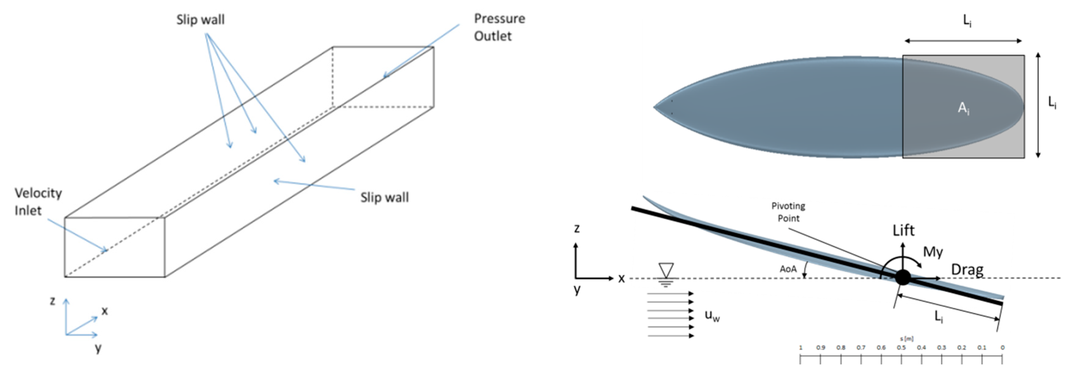
For each time step, the forces on the model are calculated by pressure integration on the wetted surface area. The domain width is 30 m, the depth is 10 m and the length is 200 m. The boundary conditions used in the simulation are represented in Figure 1: slip wall conditions were used at the bottom, at the sides and at the top and a pressure outlet boundary condition was used at the outlet. A relaxation area, consisting of an added damping domain with a flat bottom, 200 m long and discretized with stretched cells in the x-direction was added at the end of the domain in order to reduce numerical reflection from the outlet. A trimmed meshing technique was chosen in order to correctly model the water free surface in the numerical basin. Different levels of grid refinements were used in order correctly reproduce the perturbations to the free surface induced by the models.
The surface mesh was created using 100 points per curvature. The surface mesh consisted of 10 layers of prismatic mesh, with a growing factor of 1.5. To correctly model the boundary layer, the first cell height was chosen to keep the wall y+ lower than 5 on the whole surface. The convective Courant number is defined here as:
In the above equation, uw is the water flow velocity, Δt is the physical time step and Δx is the cell with in the x direction. The time step was chosen so that CCN = 0.5 in the finer portion of the grid, which is the necessary condition for the numerical stability of the VOF model.
A preliminary grid dependency study was carried out for AoA = 4 deg and U = 3.5 m/s in order to ensure numerical convergence. The plot shows a clear grid convergence with minimal differences between the middle refined grid consisting of 1.2 million cells and the fine grid which consists of 2.1 million cells. The fine grid was eventually used in the simulations. In the manoeuvring simulations, the movement of the surfboard in the domain was made possible by an overset grid approach.
2.1. Numerical Models
Three different surfboard Computer Aided Design (CAD) models are used in the present study. All of them have an initial immersed length Li = 0.5 m and oriented with an angle of attack (AoA) from the calm-water free-surface, as represented in Figure 1. The model is assumed to travel at a constant forward speed U on the water surface, which is assumed to be an incompressible fluid of density ρw and kinematic viscosity νw and it represents the liquid phase of the mixture. The traveling velocity is modelled by imposing a velocity boundary condition at the inlet boundary, meaning that the velocity uw = U is prescribed to each of the boundary cells included in the liquid phase of the mixture.
The second phase of the mixture is assumed to be air and it is modelled as an incompressible gas of density ρa and kinematic viscosity νa and zero speed (Ua = 0). The flow velocities are chosen in order to be representative for paddling speed (U = 4 m/s) and cruising speed (U = 8 m/s).
Surfboards
The surfboard models used are designed with Akushaper [11]. The models do not include fins and have a length of 1.83 m (6′0″) and a width of 0.5 m. The board geometrical parameter are in Table 1.
The baseline surfboard is a squash tail board. The LR board has the same design in terms of geometry, volume and weight, but with less rocker. The PT board has the same geometry of the baseline board but has a round tail instead of a squash tail.
3. Results and Discussion
As already mentioned, both static and dynamic simulations were performed. In the static simulations the board has a fixed position in space, and different results were obtained for a set of AoA, ranging from 2 deg to 12 deg. In the dynamic simulations, a simple maneuver representing a bottom turn is simulated. The non dimensional coefficients for lift and drag are calculated relative to the direction of motion, with the drag being along the x-axis and parallel to uw and the lift along the y-axis and perpendicular to the velocity uw. The pivoting point around which the models rotate was placed at Li = 1.5 m. The nondimensional coefficients for lift and drag force can be expressed as follows:
In the static case, the submerged area Ai [m2] was 0.185 m2 and 0.182 m2 respectively for the Baseline and LR surfboards and for the PT surfboard. While results for the static simulations are presented in form of force coefficients, the output of maneauvering simulations is expressed in form of forces since the wetted area is difficult to measure.
3.1. Static Simulations
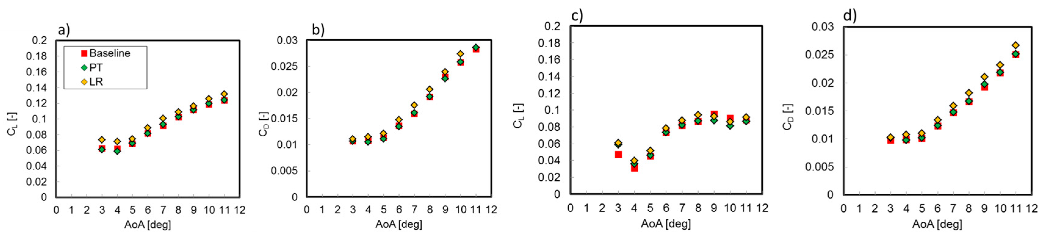
In Figure 2, the lift and drag coefficients from the static simulation is presented. From the plots, only small differences between the three boards can be noticed. In general the LR board always experiences slightly higher drag and higher lifts, which is expected due to the flatter bottom. Similar results are presented in [4] where an alaia board with a flat bottom is compared with a modern board. For a speed of 8 m/s, the PT board experiences a small drop in lift at higher angles of attack, probably due to the more tapered shape.
InFigure 3, the pressure distribution on the middle line of the board for the three boards is plotted. Minimal differences are noticeable on the 4 m/s case while larger difference can be seen on the 8 m/s case. At this speed, the LR surfboard generally experiences larger pressures and thus higher forces. The pressure peak is placed at s = 0.72 m and it is constant for all the tested boards and for all the AoA. This allows the surfer to operate and direct the board more easily. In fact, the surfer can change the AoA by moving his body forward or backwards. In principle, by lowering the AoA, the board will experience less drag and its speed will increase while pushing on the tail will allow the surfer to brake. Increasing the AoA will lead to a steep increase in lift which will allow the board to emerge from the water, moving the pivoting point further back on the board but this behavior is not treated in the current paper. If the pressure peak is constant with AoA, the surfer can move his body to change the AoA without losing balance.
3.2. Maneuvers Simulations
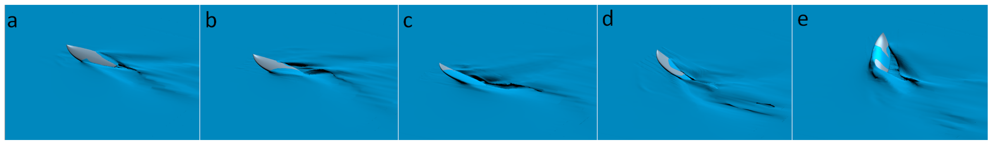
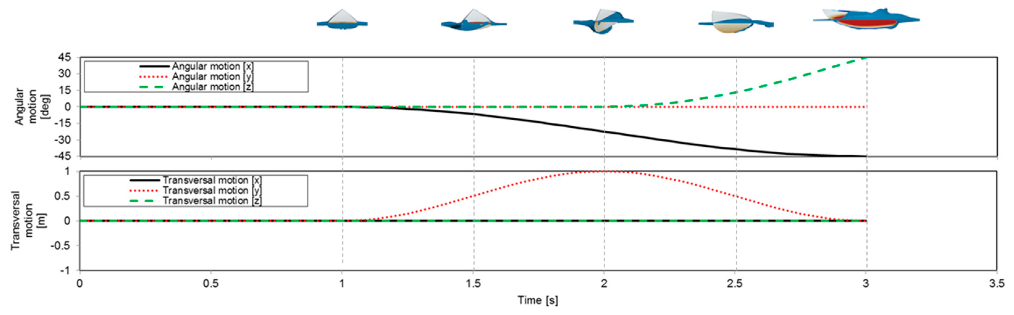
The maneuvering simulations were carried out imposing a trajectory to the board. The board was allowed to move only on three of the six degrees of freedom (DOF) (angular motion x, angular motion z-and transversal motion y) while the remaining three DOFs were kept locked. The trajectory was chosen to resemble a bottom turn at 8 m/s and it’s presented in Figure 4, Figure 5 and Figure 6. Initially the board is going straight, inclined with a AoA = 5 deg, in the second phase at t = 1 s, the board slides to the right and inclines on the x-axis while still advancing on the water (a) reaching its maximum inclination at t = 2 s (c), at this point the board rotates on the vertical axis as well ( z-axis) and begins to curve, exposing a larger part of the bottom deck to the water and thus generating larger forces and reaching its maximum inclination at t = 3 s (e).
Figure 6 shows the
forces experienced by the board in the basin reference system, from t = 0
s to t = 1 s. The board, which is inclined with a AoA = 5 deg,
only experiences vertical and horizontal forces. At t = 1 s the board
begins to translate in the y direction and to rotate along the x axis,
generating larger forces not only in the x and z-direction but also in
the y direction, due to the transversal motion. At t =2 s the board is
parallel to the flow and in a neutral position, where only horizontal and
vertical forces are acting on the board. When the turn on the z-axis
starts, a larger part of the bottom deck is exposed and consequently larger
forces are generated. The maneuvering simulations show a similar behavior to
the static simulations, where the LR board always experiences slightly larger
forces in the three directions (x, y, z) than the baseline
and PT models.
4. Conclusions
CFD simulations proved to be a useful tool and to evaluate and compare the performances of different surfboards with minimal differences in design. In particular, the simulations was able to shed light into very subtle performance differences between the different boards, which would be otherwise impossible to measure in an open field test.
Among the tested designs, the rocker affected the surfboard performances more than the tail. Flatter table bottoms induced a larger wetted area, which in return led to a higher drag but also higher lift. However, this makes flatter boards less maneuverable in the curves.
Conflicts of Interest
The authors declare no conflict of interest.
References
- Warshaw, M. The History of Surfing; Chronicle Books: San Francisco, CA, USA, 2010. [Google Scholar]
- Heimann, J. Surfing; Publisher: Taschen, Køln, Germany, 2010; (accessed on 21 August 2017). [Google Scholar]
- Kramer, M.R.; Maki, M.J.; Young, Y.L. Numerical prediction of the flow past a 2-D planing plate at low Froude number. Ocean Eng. 2013, 70, 110–117. [Google Scholar] [CrossRef]
- Oggiano, L. Numerical comparison between a modern surfboard and an alaia board using Computational Fluid Dynamics (CFD). In Proceedings of the 5th International Congress on Sport Sciences Research and Technology Support—icSPORTS, Madeira, Portugal, 30–31 October 2017; SCIPRESS: Zurich, Switzerland, 2017. [Google Scholar]
- Hirt, C.W.; Nichols, B.D. Volume of Fluid (VOF) Method for the Dynamics of Free Boundaries. J. Comput. Phys. 1981, 39, 201–225. [Google Scholar] [CrossRef]
- Ubbink, O. Numerical Prediction of Two Fluid Systems with Sharp Interfaces. Ph.D. Thesis, the University of London and Diploma of Imperial College, London, UK, 1997. [Google Scholar]
- Ferziger, J.H.; Peric, M. Computational Methods for Fluid Dynamics; Springer: London, UK, 2001. [Google Scholar]
- Menter, F.R. Two-equation eddy-viscosity turbulence models for engineering applications. AIAA J. 1994, 32, 1598–1605. [Google Scholar] [CrossRef]
- Zaïdi, H.; Fohanno, S.; Taiar, R.; Polidori, G. Turbulence model choice for the calculation of drag forces when using the CFD method. J. Biomech. 2010, 10, 405–411. [Google Scholar] [CrossRef] [PubMed]
- Wilcox, D.C. Turbulence Modelling for CFD, 3rd ed.; DCW Industries: La Canada, CA, USA, 2006. [Google Scholar]
- Aku-Shaper. Available online: https://www.akushaper.com/ (accessed on 21 August 2017).
Figure 1.
Boundary conditions (left) and side and top view of the surfboard models used in the simulations (right).
Figure 1.
Boundary conditions (left) and side and top view of the surfboard models used in the simulations (right).

Figure 2.
Drag coefficient cD versus Angle of Attack AoA for baseline, PT and LR models at 4 m/s (a,b) and 8 m/s (c,d). Baseline in red (■) and PT in green (♦) and LR in yellow (♦).
Figure 2.
Drag coefficient cD versus Angle of Attack AoA for baseline, PT and LR models at 4 m/s (a,b) and 8 m/s (c,d). Baseline in red (■) and PT in green (♦) and LR in yellow (♦).

Figure 3.
Pressure on the middle line of the surfboard bottom. Baseline in red (■) and PT in green (♦) and LR in yellow (♦) for 4m/s (a) and 8m/s (b).
Figure 3.
Pressure on the middle line of the surfboard bottom. Baseline in red (■) and PT in green (♦) and LR in yellow (♦) for 4m/s (a) and 8m/s (b).

Figure 4.
Snapshots of the free surface behind the board at different moments in the maneuvering simulation.
Figure 4.
Snapshots of the free surface behind the board at different moments in the maneuvering simulation.

Figure 5.
Imposed motion in the maneuvering simulation.

Figure 6.
Forces from the maneuvering simulation.


Table 1.
Design parameters.
| Title 1 | h1 | h2 | h0 | Li | Length | Tail Type |
|---|---|---|---|---|---|---|
| [m] | [m] | [m] | [m] | [m] | [-] | |
| Baseline | 0.105 | 0.05 | 0.02 | 0.5 | 1.85 | Squash |
| LR | 0.100 | 0.05 | 0.02 | 0.5 | 1.85 | Squash |
| PT | 0.105 | 0.05 | 0.02 | 0.5 | 1.85 | Round |
Publisher’s Note: MDPI stays neutral with regard to jurisdictional claims in published maps and institutional affiliations. |
© 2018 by the authors. Licensee MDPI, Basel, Switzerland. This article is an open access article distributed under the terms and conditions of the Creative Commons Attribution (CC BY) license (https://creativecommons.org/licenses/by/4.0/).
Share and Cite
MDPI and ACS Style
Oggiano, L.; Pierella, F. CFD for Surfboards: Comparison between Three Different Designs in Static and Maneuvering Conditions. Proceedings 2018, 2, 309. https://doi.org/10.3390/proceedings2060309
AMA Style
Oggiano L, Pierella F. CFD for Surfboards: Comparison between Three Different Designs in Static and Maneuvering Conditions. Proceedings. 2018; 2(6):309. https://doi.org/10.3390/proceedings2060309
Chicago/Turabian StyleOggiano, Luca, and Fabio Pierella. 2018. "CFD for Surfboards: Comparison between Three Different Designs in Static and Maneuvering Conditions" Proceedings 2, no. 6: 309. https://doi.org/10.3390/proceedings2060309