Flow Visualisation around Spinning and Non-Spinning Soccer Balls Using the Lattice Boltzmann Method †
by
 , ,
, ,
Takeshi Asai
1,*, 
Sungchan Hong
1 ,
,
Kaoru Kimachi
2,
Keiko Abe
3,
Hisashi Kai
3 and
Atsushi Nakamura
4 1
Faculty of Health and Sports Sciences, University of Tsukuba, Tennodai 1-1-1, Tsukuba City, Ibaraki 305-8574, Japan
2
Doctoral Program of Coaching Science, University of Tsukuba, Tennodai 1-1-1, Tsukuba City, Ibaraki 305-8574, Japan
3
Exa Japan Inc., Takashima 1-1-2, Nishi-ku, Yokohama City, Kanagawa 220-0011, Japan
4
School of Biomedicine, Far Eastern Federal University, 8 Sukhanova St., Vladivostok 690090, Russia
*
Author to whom correspondence should be addressed.
†
Presented at the 12th Conference of the International Sports Engineering Association, Brisbane, Queensland, Australia, 26–29 March 2018.
Proceedings 2018, 2(6), 237; https://doi.org/10.3390/proceedings2060237
Published: 12 February 2018
(This article belongs to the Proceedings of The 12th Conference of the International Sports Engineering Association)
Abstract
:The drag and lift of footballs have been mainly measured by wind tunnel tests. In the present study, computational fluid dynamics (CFD) and the lattice Boltzmann method were used to visualise the wakes of spinning and non-spinning footballs and analyse the dynamics of the observed vortex structures. The dominant vortex structures in the wakes of the footballs were determined to be large-scale counter-rotating vortex pairs. The fluctuation of the vortex pair for the spinning football was also estimated to be smaller and more stable than that for the non-spinning football. Although the presence of an unstable, large-scale counter-rotating vortex pair in the wake of a non-spinning ball has been previously observed in wind tunnel tests, the present study particularly found that the dominant vortex structure of a spinning ball was a stable, large-scale counter-rotating vortex pair.
1. Introduction
The drag and lift of non-spinning balls measured in previous studies related to the aerodynamic characteristics of footballs have revealed the existence of a drag crisis [1,2,3]. Spinning balls were considered in these studies because they were relatively easy to implement in the utilised wind tunnel tests. Similar tests have been conducted on spinning balls to measure their Magnus force and trajectory [3,4,5]. Attempts have also been made to measure the aerodynamic characteristics of footballs by free flight tests that closely approximate the actual processes [6,7]. These previous studies mostly involved measurement of the forces such as the drag and lift that act on the ball. Few studies have utilised visualisation and analysis of the flow and vortex structure around the ball, by which the forces acting on the ball are actually generated [8]. Furthermore, the spinning of a football during a curved shot or pass, as often occurs during competitive football games, is one of the important issues for clarifying the aerodynamic characteristics and the flow and vortex structure around a spinning football.
Computational fluid dynamics (CFD) can be used to visualise and analyse the flow and vortex structure around a bluff body, especially a steady-state analysis using turbulence models such as the k-ε model [9,10]. Nevertheless, a method for applying CFD to unsteady-state analysis using the lattice Boltzmann method was more recently developed. Some studies have also been conducted on improving the analysis precision [11,12]. In addition, the availability of powerful computing resources has increased the analysis capability for high Reynolds numbers. It is now possible to implement large eddy simulations (LESs), very-large eddy simulations (VLESs), and detached eddy simulations (DESs) [13], which facilitate more detailed descriptions of the vortex structure; as well as direct numerical simulations (DNSs) [14] without using a turbulence model.
In the present study, VLESs based on the lattice Boltzmann method were used to visualise and analyse the drag, side, and lift forces that act on a spinning football, as well as the flow around the ball. The purpose was to clarify the aerodynamic characteristics and vortex structure.
2. Methods
A three-dimensional model of the football considered in this study (Brazuca; Adidas; Figure 1) was constructed using data obtained from a 3D laser scanner (AICON 3D; Breuckmann GmbH, Meersburg, Germany).The orientation of the ball surface features (the pattern) was employed as the high symmetricity orientation from outer flow direction. For the spinning ball cases, the flow at the velocity inlet was set to a Reynolds number (Re) of 4.25 × 10⁵, which corresponds to a speed of 28 m/s, and the spinning rates of the ball were defined as 25.1, 50.2, and 75.4 rad/s (4, 8, and 12 rps), respectively. For the non-spinning cases, the flows at the velocity inlet were set to Re values of 1.25 × 10⁵ (8.2 m/s), 2.8 × 10⁵ (19.0 m/s), and 4.0 × 10⁵ (27.0 m/s). A Cartesian grid was used to generate a spatial grid of size 20 × 20 × 40 m (W × H × L) comprising nearly 500 million cells (Figure 2). A sectional grid scale technique was employed with minimum and maximum scales of 1 and 4 mm, respectively, for the spinning cases. For the non-spinning cases, minimum scales of 1.63 × 10⁻¹, 7.13 × 10⁻², and 5.02 × 10⁻² mm were employed for Re values of 1.25 × 10⁵, 2.80 × 10⁵, and 4.00 × 10⁵, respectively, with a maximum scale of 4 mm. Although these grid structures could not be used to perfectly represent the detailed vortex scales including the Kolmogorov length scale (Table 1), it was adopted because of the limitations of the available computing resources [15]. The pressure outlet was defined by 1013.25 hPa (i.e., atmospheric pressure). A no-slip boundary condition was assumed for the wall of the football, while slip was considered for the other walls including the ground surface.
Aerodynamic simulations were performed using a commercial CFD software (PowerFLOW 5.1, Exa Inc., Oak Harbor, WA, USA) and the lattice Boltzmann method. For the spinning cases, the boundary layer was simulated by a sliding mesh technique. The turbulence was modelled based on the principle of a very-large eddy simulation (VLES), which enables direct simulation of resolvable flow scales. Conversely, the unresolved scales were modelled using the re-normalisation group form of the k-epsilon equations with proprietary extensions, to achieve time-accurate physics in the VLES. The lattice of the solver was composed of voxels, which are three-dimensional cubic cells, and surfels, which are surface elements that occur where the surface of a body intersects a fluid. For the non-spinning cases, direct numerical simulation (DNS) without using a turbulent model was employed.
The average drag, lift, and side forces of the football model were calculated from the unsteady drag, lift, and side forces over a period of 1.0 s (The calculation is set to 0.2 s to 1.2 s). The following parameters were further calculated from the CFD and experimental data collected over a range of conditions: the wind velocity (U); the force acting in the opposite direction of the wind (i.e., the drag D); the force acting perpendicularly to the wind direction (i.e., the lift L); and the force acting sideways (S) (i.e., the Magnus force) with respect to the frontal view. The aerodynamic forces determined by CFD and experiment were converted into the drag coefficient (Cd), lift coefficient (Cl), and side-force coefficient (Cs) using Equations (1)–(3).
Here, ρ is the density of air (1.2 kg/m3), U is the flow velocity (m/s), and A is the projected area of the football (given by πR2, where R is the radius of the football). Cd is measured in the +X direction, Cl is measured in the +Z direction and Cs is measured in the +Y direction.
The ratio of the peripheral velocity to the velocity through the air was denoted by Sp and calculated using Equation (4).
where ω is the angular velocity of the football in radians per second (rad/s), and R is the radius of the football (0.11 m). An F-test was used to statistically test the standard deviations of the Cs values of the spinning and non-spinning balls.
Sp = ωR/U
3. Results
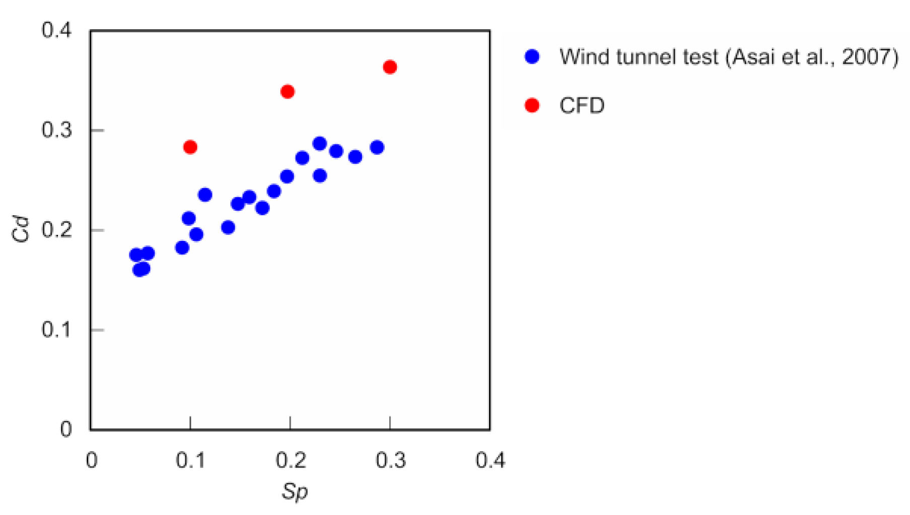
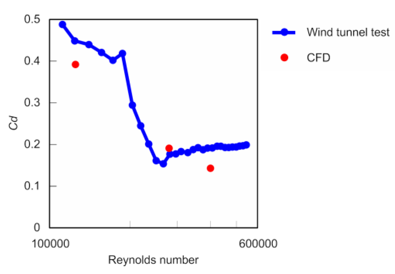
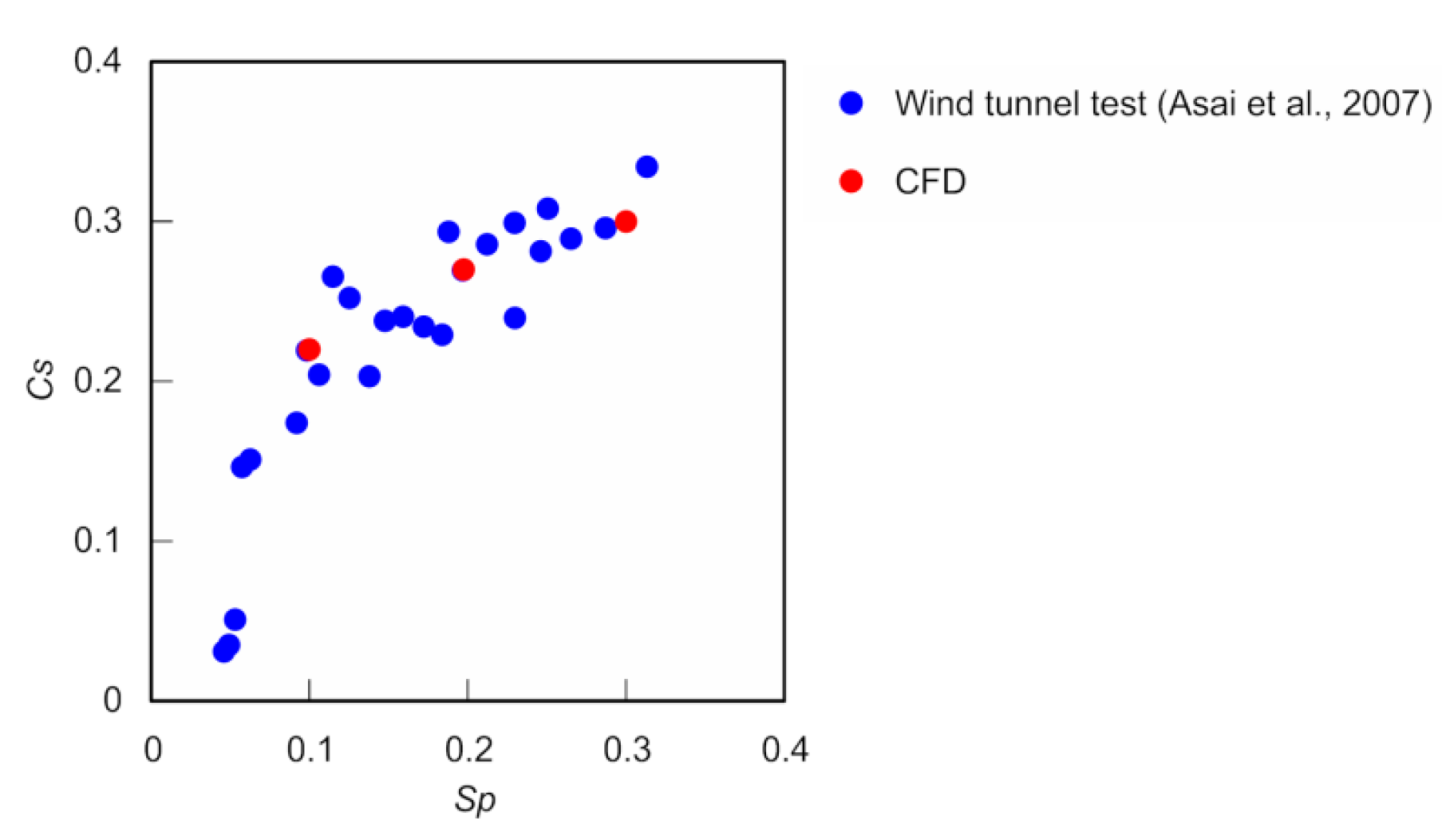
Based on the VLES results, the average Cd of the spinning ball was determined to be approximately 0.28 for Sp = 0.1, 0.34 for Sp = 0.2, and 0.36 for Sp = 0.3 (Figure 3). Based on the DNS results, the average Cd value for the non-spinning ball was determined to be approximately 0.39 for Re = 1.25 × 10⁵ in the subcritical region, 0.19 for Re = 2.80 × 10⁵ in the supercritical region, and 0.14 for Re = 4.00 × 10⁵ (Figure 4). The turbulence value of this wind tunnel test was 0.1% or less, that of CFD was defined for 0.1%. The VLES results also produced an average Cl for the spinning ball of approximately 0.22 for Sp = 0.1, 0.27 for Sp = 0.2, and 0.30 for Sp = 0.3 (Figure 5). The average Cl for the spinning ball thus tended to increase with increasing Sp.
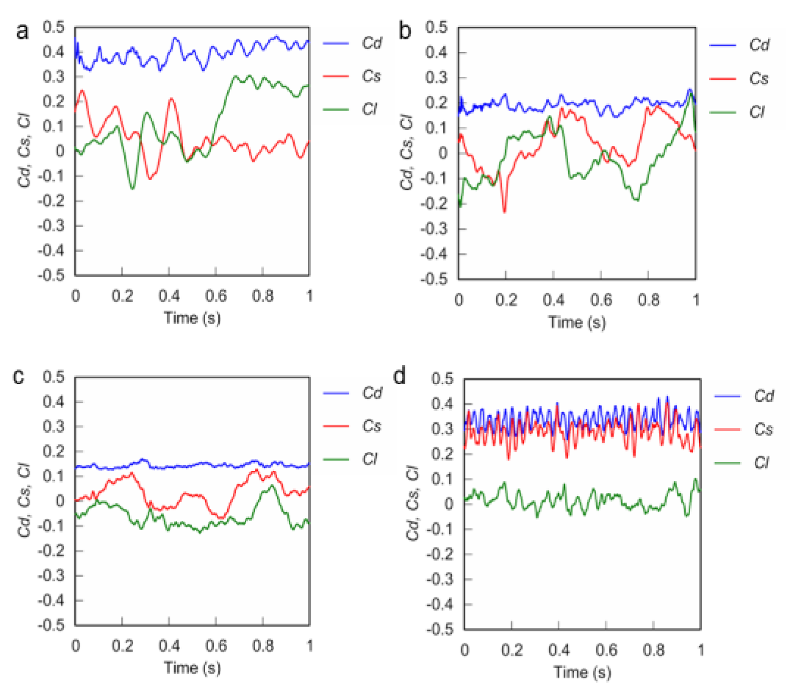
In the DNS of the non-spinning ball, for Re values of 1.25 × 10⁵, 2.80 × 10⁵, and 4.00 × 10⁵, both the unsteady state Cs and Cl tended to vary more significantly compared to Cd (Figure 6a–c). In contrast, for an angular velocity of 50.2 rad/s (8 rps) and Re of 4.25 × 10⁵ (28 m/s), there were only small fluctuations of all of Cs, Cl, and Cd (Figure 6d). In addition, the fluctuations of the unsteady-state Cs and Cl for the spinning ball were particularly smaller than those for the non-spinning ball.
Large-scale counter-rotating vortex pairs were observed to be frequently generated in the wake of the non-spinning ball. Unstable fluctuation of vortex pair was also observed in the rotation of the ball about the axis in the motion direction [16] and the breakdown (Figure 7a–c). In the VLESs, large-scale counter-rotating vortex pairs were formed in the wake of the spinning ball (ω = 50.2 rad/s, Re = 4.25 × 10⁵) on the downstream side of the rotation direction. The vortex pairs tended to be relatively stable with only small fluctuations (Figure 7d–f). The separation line of the boundary layer and the pressure distribution on the ball with respect to the axis of the motion direction were also observed.
The standard deviations of the unsteady-state Cs for the non-spinning ball were determined to be 0.078 for Re = 1.25 × 10⁵, 0.090 for Re = 2.80 × 10⁵, and 0.051 for Re = 4.00 × 10⁵, whereas in the case of the spinning ball, they were 0.046 for Sp = 0.1, 0.036 for Sp = 0.2, and 0.048 for Sp = 0.3. The standard deviation of the unsteady-state Cs was thus generally significantly smaller for the spinning ball (p < 0.01).
4. Discussion
In this study, we investigated the aerodynamic characteristics of a spinning football by CFD analysis using the lattice Boltzmann method. For comparison, CFD analysis of a non-spinning football was also conducted. The dominant vortex structures in the wake of the balls were observed to consist of large-scale counter-rotating vortex pairs, which were formed in the wake of the balls, with the Cs and Cl of the spinning ball tending to vary less than those of the non-spinning ball.
The DNSs produced an average Cd of the non-spinning ball comparable to that determined by previous wind tunnel tests [1], indicating that the present calculations were reasonable. In addition, the VLESs produced an average Cs of the rotating ball only slightly larger than that determined by previous wind tunnel tests [1].
The large-scale counter-rotating vortex pairs observed from the CFD results were found to deflect the separation line of the boundary layer and the pressure distribution on the ball. The vortex pairs are thus considered to be one of the causes of the side (lift) force that acted on both the non-spinning and spinning balls. The vortex pairs in the wake of the spinning ball (curve) tended to be stable, whereas those in the wake of the non-spinning or slowly spinning ball tended to be unstable, exhibiting large fluctuations such as rotation about the axis in the motion direction and breakdown. These instabilities are considered to be one of the causes of the knuckling effect observed in non-spinning and slowly spinning balls [17,18,19]. In addition, the deviation of side force coefficient of the spinning ball determined by CFD tended to be smaller than that of the non-spinning ball. The standard deviation of the side force coefficient of the spinning ball was also significantly smaller than that of the non-spinning ball (p < 0.01), indicating a smaller fluctuation of the side force coefficient of the spinning ball. The side force (lift) was deduced to be generated by the large-scale counter-rotating vortex pairs formed in the wake of the ball, similar to the effect of a wing tip vortex on an aircraft [20]. The stability of the counter-rotating vortex pairs in the wake of the spinning ball is thus considered to be the reason for the stability of the side force coefficient (or lift coefficient). The continuous spin of the ball is also thought to delay the stable separation of the boundary layer on the same side of the wake, thus reducing the unsteadiness of the vortex pair structure.
The present study used VLES for the CFD analysis of the spinning ball, and DNS for the non-spinning ball. The Kolmogorov minimum vortex scale [15] was, however, not calculated. In addition, further study using more powerful computing resources and analysis models with higher resolutions is required for a more detailed examination of the vortex structures and their stability. We expect that the orientation of the ball surface features (the pattern) affect the Cd, Cs, Cl for the spinning and the non-spinning cases. However, we calculated all cases in this study using only one surface orientation. Therefore, that is an important subject for future analysis.
5. Conclusions
In this study, we investigated a spinning football by CFD analysis using the lattice Boltzmann method. Through VLESs, the average Cd of the spinning ball was determined to be approximately 0.28 for Sp = 0.1, 0.34 for Sp = 0.2, and 0.36 for Sp = 0.3, while the average Cl was determined to be approximately 0.22 for Sp = 0.1, 0.27 for Sp = 0.2, and 0.30 for Sp = 0.3. VLES visualisation also revealed the frequent occurrence of large-scale counter-rotating vortex pairs in the wake of the spinning ball, and this constituted the dominant vortex structures. The vortex pairs are considered to be the cause of the observed asymmetric pressure distribution and side force on the ball. The large-scale fluctuation of the side force (Magnus force) on the spinning ball was also determined to be smaller than that for the non-spinning ball, and this is considered to produce a more stable trajectory of the former (i.e., a smooth curve).
Conflicts of Interest
The authors declare no conflict of interest associated with this manuscript.
References
- Asai, T.; Seo, K.; Kobayashi, O.; Sakashita, R. Fundamental aerodynamics of the football. Sports Eng. 2007, 10, 101–109. [Google Scholar] [CrossRef]
- Alam, F.; Chowdhury, H.; Moria, H.; Fuss, F.K.; Khan, I.; Aldawi, F.; Subic, A. Aerodynamics of contemporary FIFA soccer balls. Procedia Eng. 2011, 13, 188–193. [Google Scholar] [CrossRef]
- Passmore, M.; Rogers, D.; Tuplin, S.; Harland, A.; Lucas, T.; Holmes, C. The aerodynamic performance of a range of FIFA-approved footballs. Proc. Inst. Mech. Eng. Part P J. Sports Eng. Technol. 2011, 226, 61–70. [Google Scholar] [CrossRef]
- Goff, J.E.; Carré, M.J. Trajectory analysis of a football. Am. J. Phys. 2009, 77, 1020–1027. [Google Scholar] [CrossRef]
- Goff, J.E.; Kelley, J.; Hobson, C.M.; Seo, K.; Asai, T.; Choppin, S.B. Creating drag and lift curves from soccer trajectories. Eur. J. Phys. 2017, 38, 044003. [Google Scholar] [CrossRef]
- Carré, M.J.; Asai, T.; Akatsuka, T.; Haake, S.J. The curve kick of a football II: Flight through the air. Sports Eng. 2002, 5, 193–200. [Google Scholar] [CrossRef]
- Goff, J.E.; Smith, W.H.; Carré, M.J. Football boundary-layer separation via dust experiments. Sports Eng. 2011, 14, 139–146. [Google Scholar] [CrossRef]
- Hong, S.; Asai, T.; Seo, K. Visualization of air flow around soccer ball using a particle image velocimetry. Sci. Rep. 2015, 5, 15108. [Google Scholar] [CrossRef] [PubMed]
- Barber, S.; Chin, S.B.; Carré, M.J. Sports ball aerodynamics: A numerical study of the erratic motion of soccer balls. Comput. Fluids 2009, 38, 1091–1100. [Google Scholar] [CrossRef]
- Pouya, J.; Patrick, K.K.; MohammadHady, M.M.; William, W.L. Computational aerodynamics of baseball, soccer ball and volleyball. Am. J. Sports Sci. 2014, 2, 115–121. [Google Scholar]
- Chen, S.; Doolen, G.D. Lattice Boltzmann method for fluid flows. Annu. Rev. Fluid Mech. 1998, 30, 329–364. [Google Scholar] [CrossRef]
- Asai, T.; Hong, S.; Ijuin, K. Flow visualisation of downhill skiers using the lattice Boltzmann method. Eur. J. Phys. 2017, 38, 024002. [Google Scholar] [CrossRef]
- Constantinescu, G.S.; Squires, K.D. Numerical investigations of flow over a sphere in the subcritical and supercritical regimes. Phys. Fluid 2004, 16, 1449–1466. [Google Scholar] [CrossRef]
- Tomboulides, A.G.; Orszag, S.A.; Karniakidis, G.E. Direct and large-eddy simulations of axisymmetric wakes. AIAA Pap. 1993, 93, 546. [Google Scholar]
- Kolmogorov, A.N. The local structure of turbulence in incompressible viscous fluid for very large Reynolds numbers. Math. Phys. Sci. 1991, 434, 9–13. [Google Scholar]
- Taneda, S. Visual observations of the flow past a sphere at Reynolds numbers between 104 and 106. J. Fluid Mech. 1978, 85, 187–192. [Google Scholar] [CrossRef]
- Asai, T.; Kamemoto, K. Flow structure of knuckling effect in footballs. J. Fluid Struct. 2011, 27, 727–733. [Google Scholar] [CrossRef]
- Murakami, M.; Seo, K.; Kondoh, M.; Iwai, Y. Wind tunnel measurement and flow visualization soccer ball knuckle effect. Sports Eng. 2012, 15, 29–40. [Google Scholar] [CrossRef]
- Mizota, T.; Kurogi, K.; Ohya, Y.; Okajima, A.; Naruo, T.; Kawamura, Y. The strange flight behaviour of slowly spinning soccer balls. Sci. Rep. 2013, 3, 1871. [Google Scholar] [CrossRef] [PubMed]
- Goverdhan, R.N.; Williamson, C.H.K. Vortex induced vibrations of a sphere. J. Fluid Mech. 2005, 531, 11–47. [Google Scholar] [CrossRef]
Figure 1.
3D scanning football model.

Figure 2.
Cartesian grid used to generate the spatial grid (W 20 × H 20 × L 40 m) for the CFD analysis. The flow is from left to right.
Figure 2.
Cartesian grid used to generate the spatial grid (W 20 × H 20 × L 40 m) for the CFD analysis. The flow is from left to right.

Figure 3.
Comparison of the drag force coefficients of a spinning ball as respectively determined by CFD analyses and wind tunnel tests [1].
Figure 3.
Comparison of the drag force coefficients of a spinning ball as respectively determined by CFD analyses and wind tunnel tests [1].

Figure 4.
Comparison of the drag force coefficients of a non-spinning ball as respectively determined by CFD analyses and wind tunnel tests [1].
Figure 4.
Comparison of the drag force coefficients of a non-spinning ball as respectively determined by CFD analyses and wind tunnel tests [1].

Figure 5.
Comparison of the side force coefficients of a spinning ball as respectively determined by CFD analyses and wind tunnel tests [1].
Figure 5.
Comparison of the side force coefficients of a spinning ball as respectively determined by CFD analyses and wind tunnel tests [1].

Figure 6.
CFD-determined drag, side, and lift force coefficients of the non-spinning football for (a) Re = 1.25 × 10⁵; (b) Re = 2.80 × 10⁵; and (c) Re = 4.00 × 10⁵; and for the spinning football for (d) Re = 4.25 × 10⁵ (8 rps).
Figure 6.
CFD-determined drag, side, and lift force coefficients of the non-spinning football for (a) Re = 1.25 × 10⁵; (b) Re = 2.80 × 10⁵; and (c) Re = 4.00 × 10⁵; and for the spinning football for (d) Re = 4.25 × 10⁵ (8 rps).

Figure 7.
Examples of the vorticities of the streamlines for the (a–c) non-spinning and (d–f) spinning footballs. The ball is spinning with a positive rotation about Z axis. The Re values for the non-spinning and spinning balls are respectively 2.80 × 10⁵ and 4.25 × 10⁵ (spin rate = 8 rps). The surface is colored by pressure coefficient whereas the streamlines are colored by vorticity. The view is from behind the ball (back view).


Table 1.
Minimum vortex size with respect to the Reynolds number.
| Reynolds Number | Kolmogorov Scale (m) | Minimum Voxel Size (m) |
|---|---|---|
| 1.25 × 10⁵ | 3.30 × 10⁻⁵ | 1.63 × 10⁻⁴ |
| 2.80 × 10⁵ | 1.80 × 10⁻⁵ | 7.13 × 10⁻⁵ |
| 4.00 × 10⁵ | 1.39 × 10⁻⁵ | 5.02 × 10⁻⁵ |
Publisher’s Note: MDPI stays neutral with regard to jurisdictional claims in published maps and institutional affiliations. |
© 2018 by the authors. Licensee MDPI, Basel, Switzerland. This article is an open access article distributed under the terms and conditions of the Creative Commons Attribution (CC BY) license (https://creativecommons.org/licenses/by/4.0/).
Share and Cite
MDPI and ACS Style
Asai, T.; Hong, S.; Kimachi, K.; Abe, K.; Kai, H.; Nakamura, A. Flow Visualisation around Spinning and Non-Spinning Soccer Balls Using the Lattice Boltzmann Method. Proceedings 2018, 2, 237. https://doi.org/10.3390/proceedings2060237
AMA Style
Asai T, Hong S, Kimachi K, Abe K, Kai H, Nakamura A. Flow Visualisation around Spinning and Non-Spinning Soccer Balls Using the Lattice Boltzmann Method. Proceedings. 2018; 2(6):237. https://doi.org/10.3390/proceedings2060237
Chicago/Turabian StyleAsai, Takeshi, Sungchan Hong, Kaoru Kimachi, Keiko Abe, Hisashi Kai, and Atsushi Nakamura. 2018. "Flow Visualisation around Spinning and Non-Spinning Soccer Balls Using the Lattice Boltzmann Method" Proceedings 2, no. 6: 237. https://doi.org/10.3390/proceedings2060237