Optimal Sensor Placement through Bayesian Experimental Design: Effect of Measurement Noise and Number of Sensors ^†

Abstract

Sensors networks for the health monitoring of structural systems ought to be designed to render both accurate estimations of the relevant mechanical parameters and an affordable experimental setup. Therefore, the number, type and location of the sensors have to be chosen so that the uncertainties related to the estimated health are minimized. Several deterministic methods based on the sensitivity of measures with respect to the parameters to be tuned are widely used. Despite their low computational cost, these methods do not take into account the uncertainties related to the measurement process. In former studies, a method based on the maximization of the information associated with the available measurements has been proposed and the use of approximate solutions has been extensively discussed. Here we propose a robust numerical procedure to solve the optimization problem: in order to reduce the computational cost of the overall procedure, Polynomial Chaos Expansion and a stochastic optimization method are employed. The method is applied to a flexible plate. First of all, we investigate how the information changes with the number of sensors; then we analyze the effect of choosing different types of sensors (with their relevant accuracy) on the information provided by the structural health monitoring system.

1. Introduction

The main goal of Structural Health Monitoring (SHM) is to obtain information on the condition of existing structures that could be subjected to damages over time and therefore make decisions on the basis of which suitable actions should be taken, e.g., repair, substitution or maintenance. Any SHM procedure can be conceptually divided into three stages:

-

choice and design of the sensor network, in terms of number, type and location of sensors to be deployed;

-

collection and storage of data from the sensor network;

-

estimation of the mechanical parameters through an appropriate mathematical method.

In this paper we focus on the first aspect, i.e., how to design the SHM system in order to maximize its usefulness and therefore minimize the uncertainty of the parameters estimation.

Several methods for the optimal placement of sensors have been proposed in the literature: for a thorough overview of the most commonly adopted methods the interested reader may refer to [1,2,3]. These methods are based on the maximization of the sensitivity of the measured quantity with respect to the mechanical parameters to be estimated; therefore the sensor accuracy cannot be taken into account in the optimization statement.

In this paper we present a Bayesian framework for quantifying the benefit of a SHM system, motivated by the work of Huan and Marzouk [4], and effectuating an optimal design in terms of type, number and position of the sensors. Moreover, having decided the type and the number of sensors it is possible to find their optimal spatial configuration. Different experimental setups are compared in order to select the one that guarantees the maximal increase in the information conveyed by the prior and posterior (after measurement) distribution of the parameters. In order to compute the optimization function, a Monte Carlo (MC) approach is exploited. For ensuring computational efficiency, the Finite Element (FEM) model used to relate the input (mechanical parameters) to the outputs (measurements) is replaced by a surrogate model, delivered via Polynomial Chaos Expansion (PCE). Lastly, since the optimization function may be characterized by local maxima, a stochastic optimization method, namely the Covariance Matrix Adaptation-Evolution Strategy (CMA-ES), has been used.

The method is applied to a benchmark case: the optimal location of sensors on a flexible plate is obtained. Moreover, we show how the information gain changes with respect to the measurement noise and the number of sensors.

2. Method

The random variables defining the problem are:

-

$y\in {ℝ}^{n_y}$ is the vector gathering the measured data, with $n_y$ denoting the number of sensors included in the SHM system;

-

$\theta \in {ℝ}^{n_{\theta }}$ is the vector of mechanical parameters to be estimated through a Bayesian approach, with $n_{\theta }$ defining the number of parameters to be estimated.

Let us define the sensors network configuration through the vector $d\in {ℝ}^{n_d}$, either in terms of spatial coordinates or node labels of the FEM model.

According to [5], the optimal design $d^{*}$ of an experiment for the Bayesian inference of $\theta$ is:

$$\mathrm{find} d^{*}=\arg \underset{d\in \mathcal{D}}{\max }{{\displaystyle \int }}_{\mathcal{Y}}^{}{{\displaystyle \int }}_{\Theta }^{}U\left(d,y,\theta \right)p(\theta ,y|d)d\theta dy$$

(1)

$\mathcal{Y}$ and $\Theta$ are respectively the supports of $p(y|d)$ and $p(\theta |d)$, while $\mathcal{D}$ is the space of all possible vectors $d$. As suggested in [6], the most used utility function $U\left(d,y,\theta \right)$ is the Kullbach-Leibler divergence, i.e., the increase in Shannon information between the prior probability distribution and the posterior probability distribution:

$$U\left(d,y,\theta \right)=\ln \left[\frac{p\left(\theta |y,d\right)}{p\left(\theta \right)}\right]$$

(2)

In other words, the KL divergence measures the increase in information due to the data acquired from the sensors. In [7], the Shannon information is computed by asymptotic approximation. The advantage of this approach is that it enables the computation of the optimization function in a closed form, while the disadvantage lies in the fact that the designer has to place a guess on $\theta$, rendering the solution valid for problems with small uncertainty. To the contrary, the approach proposed in [4] is robust with respect to $\theta$, since it only necessitates an initial guess on the prior distribution $p\left(\theta \right)$. If the designer has no prior information on the distribution of the mechanical parameters, a uniform distribution may be chosen.

Following [4], Equation (1) can be handled through a MC approximation as follows:

$$\mathrm{find} d^{*}=\arg \underset{d\in \mathcal{D}}{\max }\frac{1}{N^{out}}{{\displaystyle \sum }}_{i=1}^{N^{out}}\left\{\ln \left[p(y^i|{\theta }^i,d)\right]-\ln \left[\frac{1}{N^{in}}{{\displaystyle \sum }}_{j=1}^{N^{in}}p(y^i|{\theta }^j,d)\right]\right\}$$

(3)

$N^{out}$ and $N^{in}$ are the number of samples to be drawn.

In order to compute the likelihood function $p\left(y|\theta ,d\right)$, a forward model is required:

$$y=G\left(\theta ,d\right)+\epsilon$$

(4)

where $\epsilon$ represents the modelling and measurement error. The measurement error is assumed as a zero-mean Gaussian noise, with the standard deviation depending on the sensor type.

As shown in [8] for quasi-static loading conditions, $y$ represents the displacements or rotations measured at the sensors locations. The forward model is therefore:

$$G^{FE}\left(\theta ,d\right)=L\left(d\right)K^{-1}\left(\theta \right)F$$

(5)

where $L\left(d\right)\in {ℝ}^{n_s\times n_{dof}}$ is a Boolean matrix that selects only the degrees of freedom (DOFs) actually observed by the deployed sensors; $K\left(\theta \right)\in {ℝ}^{n_{dof}\times n_{dof}}$ is the stiffness matrix; $F\in {ℝ}^{n_{dof}}$ is the load vector; $n_s$ is the number of sensors to be deployed and $n_{dof}$ is the total number of DOFs of the system.

The likelihood function is computed as:

$$p\left(y^i|{\theta }^j,d\right)=p_{\epsilon }\left(y^i-G\left({\theta }^j,d\right)\right)$$

(6)

where $p_{\epsilon }~\mathcal{N}\left(0,{\Sigma }_{\epsilon }\right)$ is the measurement error probability distribution (${\Sigma }_{\epsilon }\in {ℝ}^{n_s}\times {ℝ}^{n_s}$ is the covariance matrix).

Since the evaluation of the optimization function in Equation (3) is characterized by a high computational cost, the forward model in Equation (5) is replaced by a surrogate model, based on Polynomial Chaos Expansion (PCE). A set of $N^{PCE}$ joint input samples ${\left[{\theta }^T d^T\right]}^{}$ is respectively drawn from $p\left(\theta \right)$ and $\mathcal{U}\left(\mathcal{D}\right)$, the output is computed through the FEM model. The surrogate model is built using the input and output set of samples, according to [9].

As the MC method has been utilized, the resulting optimization function will be noisy and a standard optimization method may fail due to the presence of local maxima. To overcome the problem, the CMA-ES [10] method is herein exploited. The PCE model is used for each iteration of the optimization procedure to compute the likelihood function in Equation (6).

3. Results

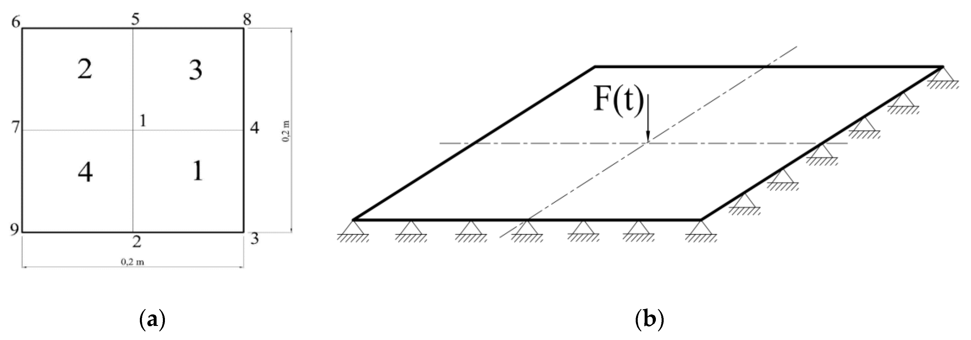
The method is now demonstrated on a simple benchmark problem. A simply supported flexible plate is subjected to a quasi-static load applied at the center (Figure 1b). It is assumed that the goal is to estimate the Young modulus of the four zones in which the structure is subdivided (Figure 1a) via use of sparse (sensor) measurements. Out-of-plane deflections are assumed as the available measurements and obtained via a numerical model built in a commercial FEM code (SIMULIA Abaqus FEA 6.13).

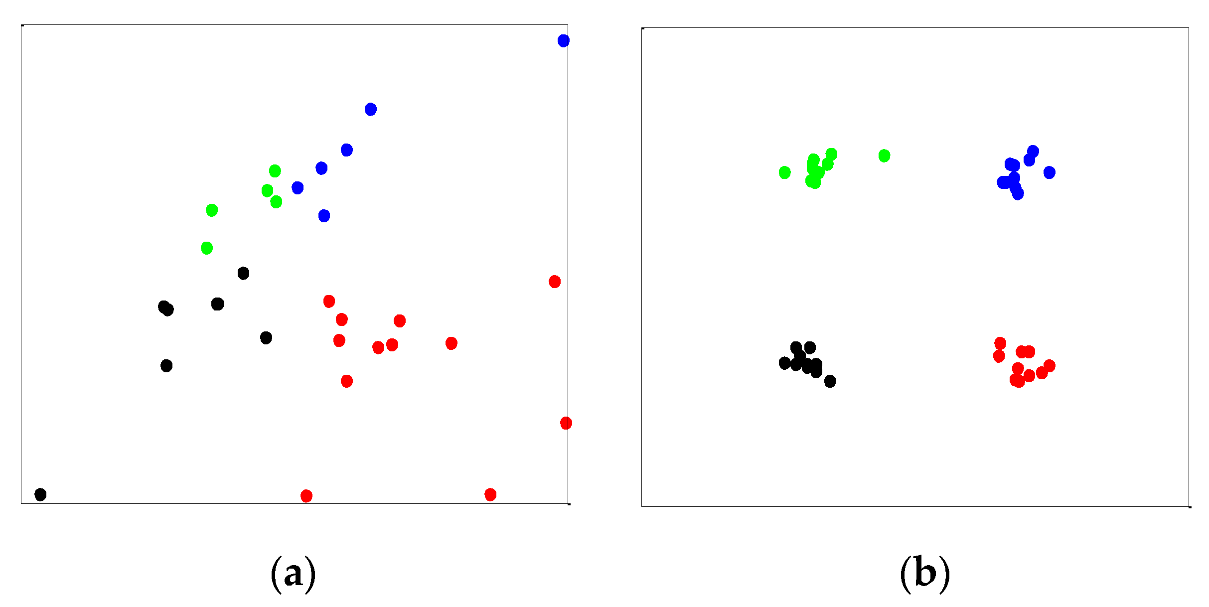
In what follows, the number of samples of the MC approximation is set as $N^{out}=N^{in}=5·{10}^3$ and the number of samples drawn to compute the PCE surrogate is $N^{PCE}=5·{10}^3$. Figure 2 displays the optimal configuration of 4 sensors over the plate. Each sensor is depicted with a different color; 10 runs of the algorithm have been performed in order to check the stability of the results. For $p\left(\theta \right)~\mathcal{U}\left[0,E\right]$ (Figure 2a), the PCE model is not able to capture the long tail in the distribution of $y$ due to the singularity condition $E=0 \mathrm{MPa}$. On the other hand, a prior distribution $p\left(\theta \right)~\mathcal{U}\left[\frac{2E}{3},E\right]$, with a lower bound far from the value $E=0 \mathrm{MPa},$ yields more stable results (Figure 2b). As expected, the optimal configuration is symmetric.

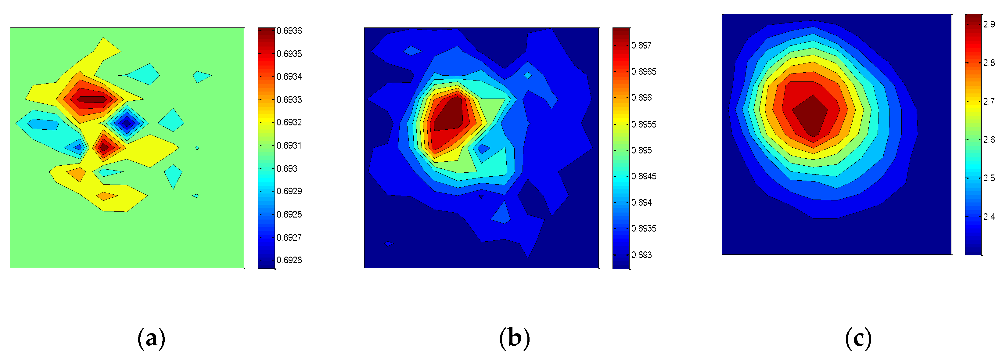
Let us consider the effect of sensor accuracy. For plotting the objective function across a range of possible design configurations $d$, we consider the simplest scenario of a single sensor $n_s=1$. In this case, the contour of the expected information gain may be plotted for each point of the plate. In Figure 3, we show that by decreasing the accuracy of the sensor, i.e., reducing the standard deviation $\sigma$ of the measurement error, the objective function becomes more scattered, even if the optimal position of the sensor remains unchanged. Moreover, we can point out that the information gain obtained for the optimal configuration increases as the accuracy of the sensor increases.

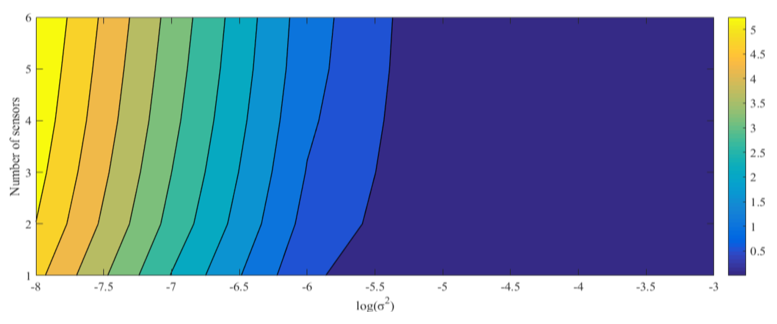
In Figure 4 the contour plot of the information gain as a function of the number of sensors and the standard deviation of the measurement error is plotted. As naturally expected, the information increases for adoption of a larger number of sensors; on the other hand, for a certain number of sensors, the information gets higher as the accuracy is increased. The black lines represent the iso-information lines. This approch can be applied to any kind of structure that has to be investigated though a SHM system and it allows to compare different design solutions of the sensor network. In this case, since the plate is a very simple structure, with high spatial correlation, the number of sensors deployed does not affect so much the information.

4. Conclusions

In the present paper a new method for the optimal placement of sensors for SHM applications has been presented.

The optimal spatial configuration of the sensor network is obtained by maximizing the expected gain in Shannon information between the prior and the posterior distribution of the parameters to be estimated. In order to compute the optimization function, a MC approximation and PCE surrogate model have been exploited.

The framework has been applied to a flexible simply supported plate: it has been shown that the choice of the prior distribution can lead to unstable solutions. The effect of the number of sensors and the measurement noise has been investigated. The information gain respectively increases as more accurate and more sensors are employed. The framework can be applied to design a SHM system, in terms of number, type and configuration of sensors as it allows to quantify the information delivered by the sensor network. Thus, different experimental designs can be compared in terms of both information and cost.

References

- Meo, M.; Zumpano, G. On the optimal sensor placement techniques for a bridge structure. Eng. Struct. 2005, 27, 1488–1497. [Google Scholar] [CrossRef]
- Leyder, C.; Ntertimanis, V.; Chatzi, E.; Frangi, A. Optimal sensors placement for the modal identification of an innovative timber structure. In Proceedings of the 1st International Conference on Uncertainty Quantification in Computational Sciences and Engineering, Crete Island, Greece, 25–27 May 2015; pp. 467–476. [Google Scholar]
- Bruggi, M.; Mariani, S. Optimization of sensor placement to detect damage in flexible plates. Eng. Optim. 2013, 45, 459–676. [Google Scholar] [CrossRef]
- Huan, X.; Marzouk, Y.M. Simulation-based optimal Bayesian experimental design for nonlinear systems. J. Comput. Phys. 2013, 232, 288–317. [Google Scholar] [CrossRef]
- Lindley, D.V. Bayesian Statistics: A Review; Society for Industrial and Applied Mathematics (SIAM): Philadelphia, PA, USA, 1972. [Google Scholar]
- Ryan, K.J. Estimating expected information gains for experimental designs with application to the random fatigue-limit model. J. Comput. Graph. Stat. 2003, 12, 585–603. [Google Scholar] [CrossRef]
- Papadimitriou, C. Optimal sensor placement methodology for parametric identification of structural systems. J. Sound Vib. 2004, 278, 923–947. [Google Scholar] [CrossRef]
- Capellari, G.; Chatzi, C.; Mariani, S. An optimal sensor placement method for SHM based on Bayesian experimental design and Polynomial Chaos Expansion. In Proceedings of the VII European Congress on Computational Methods in Applied Sciences and Engineering, Crete Island, Greece, 5–10 June 2016. [Google Scholar]
- Marelli, S.; Sudret, B. UQLab User Manual, Chair of Risk, Safety & Uncertainty Quantification; ETH Zürich: Zürich, Switzerland, 2016. [Google Scholar]
- Hansen, N.; Müller, S.D.; Koumoutsakos, P. Reducing the time complexity of the derandomized evolution strategy with Covariance Matrix Adaptation (CMA-ES). Evolut. Comput. 2003, 11, 1–18. [Google Scholar] [CrossRef] [PubMed]
Figure 1.
Benchmark case: (a) View from above, zones numbering; (b) Load and boundary condition.
Figure 2.
Optimal position of sensors, results of 10 algorithm runs. (a) ; (b) .
Figure 3.
Contour of the objective function with one sensor for each possible location on the plate with different standard deviations of the measurement noise: (a) ; (b) m; (c) m.
Figure 4.
Contour of the objective function with one sensor for different standard deviations and number of sensors.
Publisher’s Note: MDPI stays neutral with regard to jurisdictional claims in published maps and institutional affiliations. |
© 2016 by the authors. Licensee MDPI, Basel, Switzerland. This article is an open access article distributed under the terms and conditions of the Creative Commons Attribution (CC BY) license (https://creativecommons.org/licenses/by/4.0/).
Share and Cite
MDPI and ACS Style
Capellari, G.; Chatzi, E.; Mariani, S. Optimal Sensor Placement through Bayesian Experimental Design: Effect of Measurement Noise and Number of Sensors. Proceedings 2017, 1, 41. https://doi.org/10.3390/ecsa-3-D006
AMA Style
Capellari G, Chatzi E, Mariani S. Optimal Sensor Placement through Bayesian Experimental Design: Effect of Measurement Noise and Number of Sensors. Proceedings. 2017; 1(2):41. https://doi.org/10.3390/ecsa-3-D006
Chicago/Turabian StyleCapellari, Giovanni, Eleni Chatzi, and Stefano Mariani. 2017. "Optimal Sensor Placement through Bayesian Experimental Design: Effect of Measurement Noise and Number of Sensors" Proceedings 1, no. 2: 41. https://doi.org/10.3390/ecsa-3-D006