Fractal Curves from Prime Trigonometric Series


1
NIKI Ltd. Digital Engineering, Research Center, 205 Ethnikis Antistasis Street, 45500 Katsika, Ioannina, Greece
2
TWT GmbH Science & Innovation, Mathematical Research, Ernsthaldenstr. 17, 70565 Stuttgart, Germany
*
Author to whom correspondence should be addressed.
Fractal Fract. 2018, 2(1), 2; https://doi.org/10.3390/fractalfract2010002
Submission received: 10 November 2017
/
Revised: 26 December 2017
/
Accepted: 26 December 2017
/
Published: 3 January 2018
Abstract
:We study the convergence of the parameter family of series: , defined over prime numbers p and, subsequently, their differentiability properties. The visible fractal nature of the graphs as a function of is analyzed in terms of Hölder continuity, self-similarity and fractal dimension, backed with numerical results. Although this series is not a lacunary series, it has properties in common, such that we also discuss the link of this series with random walks and, consequently, explore its random properties numerically.
1. Introduction
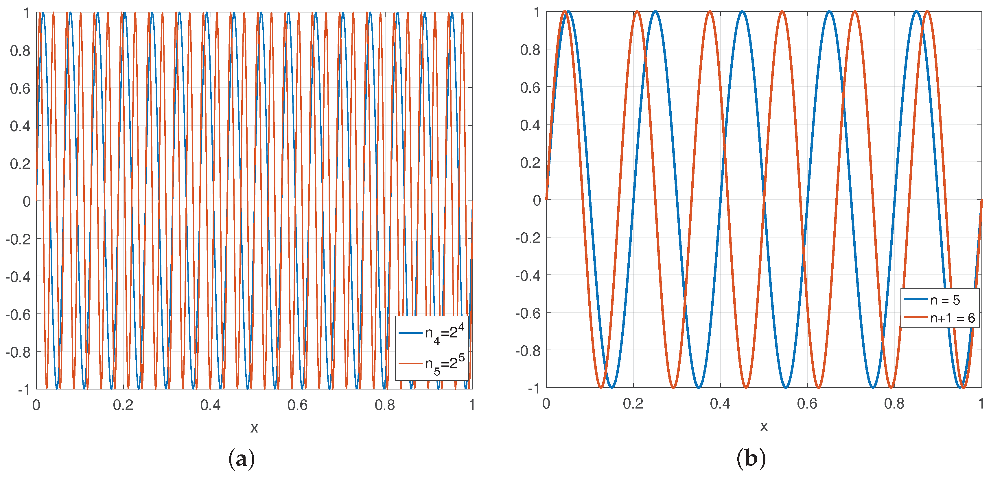
The prime numbers are not randomly distributed but, there are random models that capture important properties of the distribution of prime numbers well (e.g., [1]). The random behavior of a deterministic mathematical object can be found elsewhere: there are classical function series that can be approximated by random processes. Let us briefly describe these series: consider the two functions and for an arbitrary integer . These behave as strongly dependent random variables if we consider x to be a random real variable uniformly distributed on some interval. However, if one picks from the sequence of frequencies a sub-sequence , such that the integer sequence grows sufficiently fast, i.e., , the quantities and behave like independent random variables (see Figure 1 as an example and Section 3).
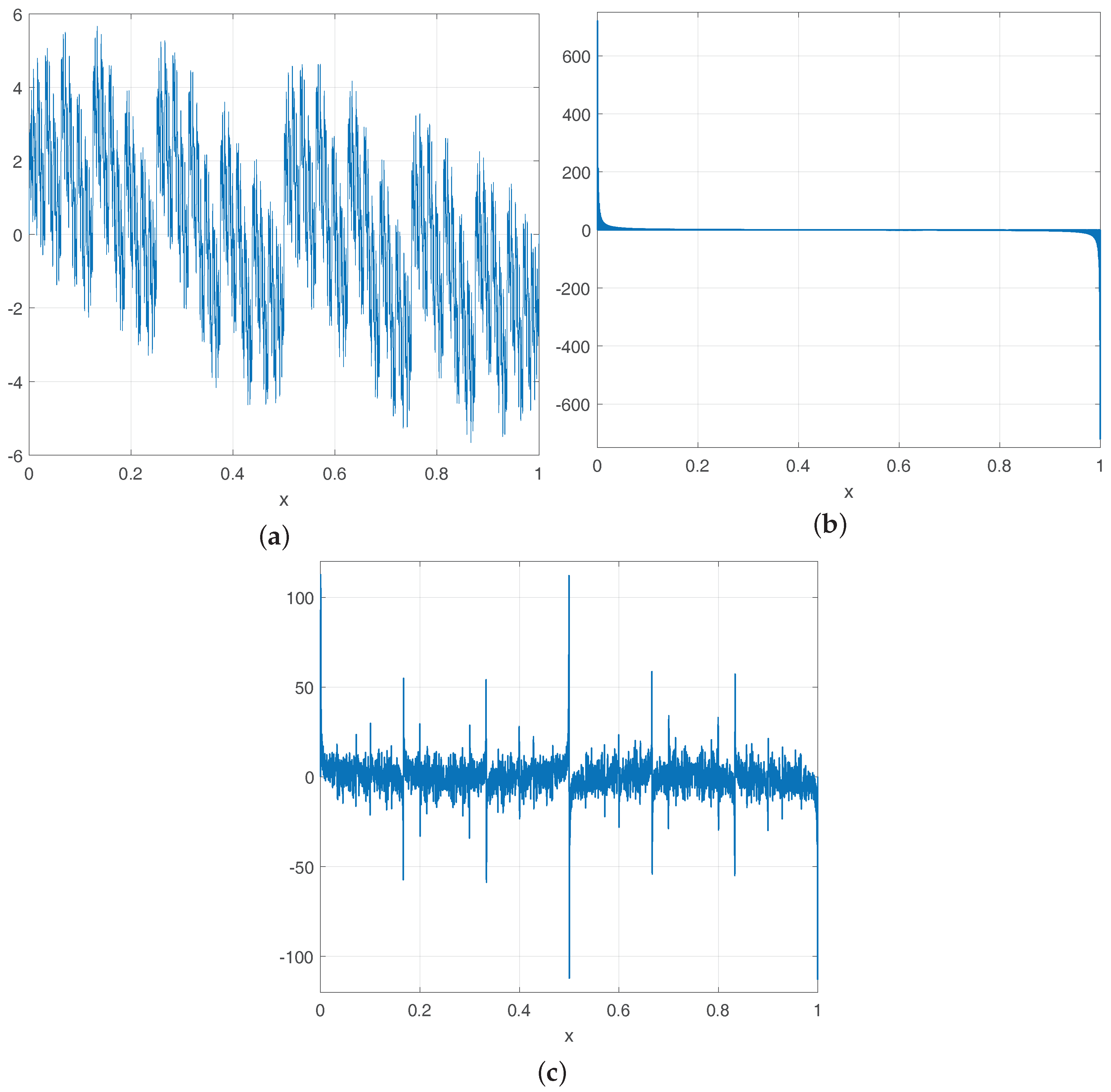
Now, one can construct a random walk out of these random variables: start at zero. At time k, move up. At time N, we find ourselves at . This sum is displayed for in Figure 2 on the left.
This example is known as a lacunary Fourier series, that is its frequencies fulfill the growth condition given above. Its random properties are a classical field of research. In the literature, the sequence of prime numbers is often cited as a counterexample for a sequence of frequencies that does not give rise to a lacunary Fourier series: it neither fulfills the growth condition nor alternative conditions on arithmetic patterns that exist in the literature. However, experiments in this article suggest that share many of the random properties of lacunary series (see Figure 2 for a first impression or [2]): for instance, the central limit theorem seems to hold. Unfortunately, this looks difficult to prove (see e.g. [3], p. 2).
On the other hand, we can look at other manifestations of randomness in lacunary series (e.g., in the example in Figure 2) and try to see if they are also present in our prime series : by introducing appropriate coefficients , the walk can be approximated by a Wiener process, which is an almost everywhere continuous random walk with independent normally-distributed increments (see [4] and Section 3). This implies directly many interesting properties for the series, e.g., the law of iterated logarithm holds. It would be interesting if a similar approximation exists for our series . Again, we were not able to prove this.
However, we can show that our series has in fact for specific properties in common with a Wiener process, e.g., its regularity and fractality (see Section 2). The above-mentioned example is in fact famous for these reasons: it belongs to the family of Weierstrass functions , which have been extensively studied for its differentiability properties. Under certain conditions on , this function is nowhere differentiable, but Hölder continuous.
Another historical example that is non-differentiable, but multifractal, is the Riemann function . Note, that it is not a lacunary series as . With our prime series, we place ourselves in between these two historical examples with respect to the growth of its frequencies.
While prime sums are extensively studied in the context of the famous prime conjectures (e.g., for Vinogradov’s theorem and the like), we have not found a treatment of trigonometric series over prime numbers. The reason for this is most probably that these series do not have the necessary form to help to progress in the proofs of the prime conjectures where prime exponential sums play a dominant role. As mentioned above, these series have not been studied in the context of lacunary series as prime numbers neither grow fast enough nor have known arithmetic properties, which are necessary for a straightforward analysis.
By using the results of prime number theory, we are nevertheless able to show conditions on the differentiability and self-similarity of our prime series. Experimentally, we explore also its box dimension in dependence of .
Remark 1.
For most of our questions, we can restrict ourselves, without loss of generality, to the real part of the series, which we denote by , as well.
2. Convergence and Differentiability
There are basically two factors that influence the smoothness and convergence of a function series as ours:
- The faster the coefficients decrease for , the smaller is the influence of the higher frequencies. This implies that the series converges better and the resulting function is smoother.
- The faster the frequencies increase or, equivalently, the greater the gaps, the smaller the period of the oscillation becomes, so that one obtains more peaks and sinks in one interval, which increases the fractal character.
2.1. Historical Remarks
The nature of these influences, easily deduced, are also backed by the long history of studies on the following two families of functions (and derived families):
Let:
be the family of Weierstrass functions, which have been extensively studied. One knows the following:
Theorem 1
2. If , then is nowhere differentiable. Further, the Hölder exponent is a constant function , i.e., for all , it holds:
On the other hand, one has the family of Riemann’s functions (whose authorship by Riemann is apparently only confirmed by Weierstrass) defined by:
which has the following proven properties:
Theorem 2
([5,7,8,9,10]). 1. If , then the series is not a Fourier series of an -function. If , then converges at x if and only if , where are coprime and four divides .
2. If , then the series converges in p-norm to a -function for .
3. If , then the series has bounded mean oscillation.
4. If , then is not differentiable at any irrational value of x, and its Hausdorff dimension for is equal to:
If , then is differentiable at x if and only if where are coprime and four divides .
5. If , the Hölder exponent is discontinuous everywhere. In fact, is a function with unbounded variation and multifractal.
In the following, we aim to give a similar description for our function series. Let us start with some preliminary definitions, which are necessary for what follows.
2.2. Preliminary Definitions
We call a function locally Hölder continuous at , if there exist and , such that:
We call the supremum of s for which these inequality holds at the local Hölder exponent.
Let be a smooth function with compact support . We write:
for the Fourier transform of . Further, let be given such that the support of its Fourier transform is contained in , then the Gabor wavelet transform of a function is defined by:
With these notation, we have the following estimation, which is a special case of Proposition 5 in [6]:
Proposition 1 (Jaffard).
Let be a bounded function. Let be the Gabor wavelet transform of f. If f is locally Hölder continuous at with Hölder coefficient s, then there exists such that for all and for all and for all , we have:
2.3. Differentiability of
In the spirit of the results in Section 2.1, we aim to determine which conditions have to be fulfilled by the coefficients and frequencies in our example in order to have a certain degree of differentiability. Firstly, we consider:
where f is any function of prime numbers. We can state the trivial fact that:
Proposition 2.
For any , if , then the partial sums converge uniformly and absolutely to a continuous function denoted by .
Proof.
We have for all p. By the Weierstrass M-test, the partial sums converge uniformly and absolutely if Using the Riemann–Stieltjes integral and the prime number theorem, we get:
where denotes the number of primes , finishing the proof. ☐
We take now
and denote with its limit whenever it exists. Then, one can show the following statement:
Theorem 3.
Let and .
- Then, the series converges uniformly and absolutely to a continuous function .
- For , if further , then the function is , i.e., m-times continuously differentiable.
Proof.
For the first result, we use the properties of the prime zeta function : it converges absolutely for and diverges for (see, e.g., [11,12]). The coefficients are an upper bound for the terms . Consequently, the Weierstrass M-test implies that for and any , converges uniformly and absolutely to . As any partial sum is continuous, the limit is a continuous function, as well.
Secondly, for any n and t, we can differentiate the partial sums:
This sequence of derivatives converges uniformly with the same argument as above for , so that one concludes that is continuously differentiable itself with derivative . By induction over m, one proves the m-time differentiability of the function. ☐
Remark 2.
The result is in accordance with the intuitive smoothness of the series: for fixed , the series becomes smoother, the smaller the frequency , , or equivalently, the larger the period. Therefore, the peaks and sinks of the oscillation are more and more separated so that the series becomes smoother (see Figure 3, Figure 4 and Figure 5).
Theorem 4.
If , then the function is Hölder continuous with Hölder coefficient .
Proof.
First of all, let be an integrable function and , then by using the Riemann–Stieltjes integral (see, e.g., [13]) and the prime number theorem as above, one knows:
From this formula and denoting the logarithmic integral function, one deduces (substituting by ) for :
Approximating the logarithmic integral, this implies:
If , we have to use the explicit formula for the prime zeta function to get an estimate for the speed of convergence (see, e.g., [14] for a derivation of the formula). We then have by partial summation:
where denotes the Riemann zeta function and the Moebius function. Therefore, we get for the tail of the prime zeta function:
Combining Equations (1) and (2) on the asymptotic of the prime zeta function, we can estimate now the regularity of our function .
For any , we choose Then, we have with the mean value theorem and using the absolute convergence of the series:
The exponent is not necessarily optimal, but a lower bound. However, it suffices to conclude that the function is Hölder continuous, so that we can derive an upper bound for its Hölder exponent.
For this step, we use a method developed by Jaffard in [6], which relies on a wavelet transform and the idea of choosing the wavelet transform such that only one frequency of is picked up. Let and .
We choose a function whose Fourier transform has compact support and . We then look at the Gabor-wavelet transform:
with . Substituting for in the equation, we get:
As the support of is a subset of the unit interval, it vanishes for any , so the expression is reduced to:
Recall that we have just proven that is locally Hölder continuous at . Further, for all m, it is and . Hence, applying Proposition 1, there exists such that for all :
The gap is bounded by from above, so that the Hölder coefficient s is bounded by from above, finishing the proof. ☐
Remark 3.
Let be fixed. The bigger the gaps of the frequency, , the stronger the irregularity of .
2.4. Self-Similarity and Fractal Dimension
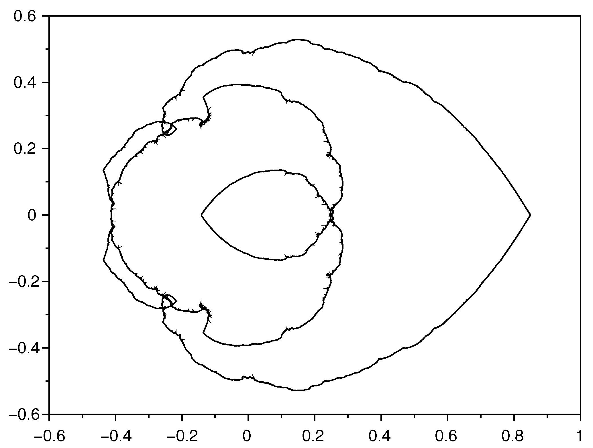
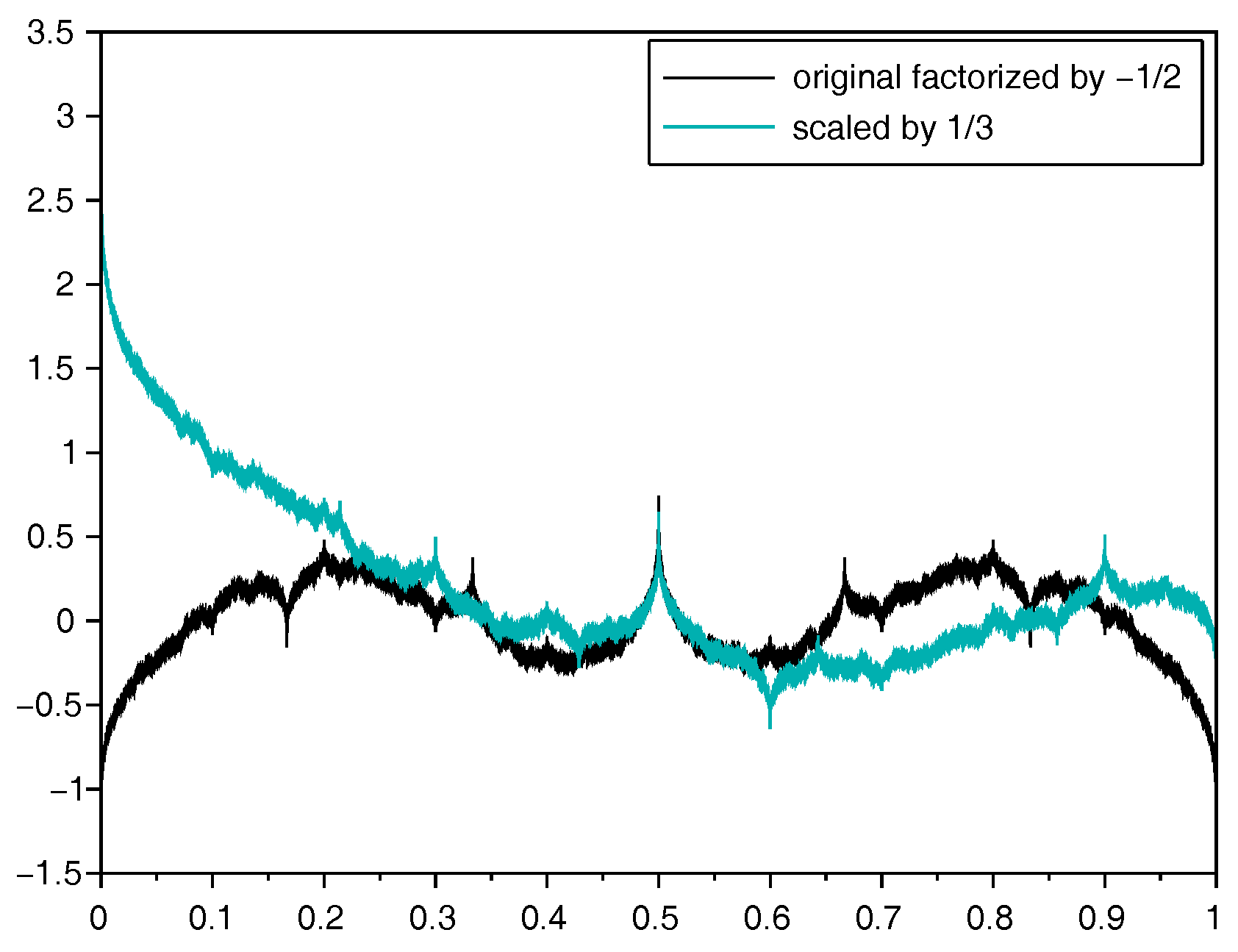
The graph of the function seems to be self-similar for certain . There seems to be an approximate scalar invariance at points , where q is prime. Let us make this intuition more precise: look for example at the partial sums in Figure 6.
Denote by the k-th prime number. We restrict ourselves again to the real part of . The point is a global minimum as and as the primes greater than two are odd. Now, consider the point : we have . More generally, one has:
That is, we can decompose the partial sum into residue classes of the prime numbers and the roots of unity of cosine. One knows that the number of primes that are congruent to are approximately the same for all l, that is , where denotes the Euler totient function and is equal to for q prime. Therefore, for any , q prime, one can use this distribution and the Riemann–Stieltjes integral to show that the difference between the sums for each converges to zero for , that is:
The factors are exactly the prime roots of unity, and the sum . Consequently, one computes:
As we have , one could argue that:
See Figure 7. However, keep in mind that these are only asymptotic equivalences, while our partial sum does not converge for all for , so the self-similarity of the graph is certainly not strict.
Fractal Dimension of
Further, we compute numerically the box dimension of the graph of defined in the following way: let be the rectangle such that the graph is contained. We compute then for the intersections . We denote the number of non-empty intersections by . The box dimension is then given by:
In accordance with our results on the regularity of , we obtain the following Figure 8 for the (numerically computed) box dimension over the fraction . For fixed and , that is , we expect that the fractal dimension converges to two. On the other hand, for , the fractal dimension should converge to one as the graph gets continuously differentiable if .
Remark 4.
In recent literature (see, e.g., [15]), the concept of the fractal dimension of prime distribution is studied: it is defined with the help of an indicator function on the natural numbers, which is one if is prime, otherwise zero. The fractal dimension is then computed as the average number of ones in randomly-chosen minors of the -matrix . In a recent publication ([16]), the self-similarity of these images (created by displaying the ones in the matrix in black, zeros in white) is also treated. These concepts are not related to the self-similarity or the fractal dimension of our series: the fractality of depends on its Hölder exponent, which relies on the exponents and on the gaps of frequencies . In this sense, it certainly depends on the prime distribution, but we do not see a direct application of the concepts cited above. More probable is that in order to analytically compute the fractal dimension, one would have to use the large sieve inequality where on the right side would appear values of .
There is clearly no reverse correlation from the fractal dimension of the graph to the prime distribution as there are other, even multifractal curves as the cited Riemann function whose frequencies are not prime sequences.
3. Random Properties for
The quite similar behavior of lacunary and random Fourier series allow us to think that it might be possible to capture the random character of the series , which is the subject of this section. Let us briefly review what is known in the context of lacunary sequences and random variables.
3.1. Lacunary Sequences Behaving as Independent Random Variables: Short Overview
The terms and behave like random variables, but strongly dependently. However, if one restricts the sequence of frequencies to where the sequence has sufficiently fast-growing gaps, i.e.,
then the sequences behave like independent random variables. For example, one has:
where is the normal distribution. This was the main observation that has led to study the connections between lacunary and random Fourier series, most importantly the question of which are the optimal growth conditions on the sequence such that the sequence for general periodic measurable functions f with vanishing integral exhibits random properties (see the historical overview in [17]). By introducing weights that obey certain growth conditions themselves, one can recover several limit theorems in complete analogy with random variables. In particular, the Central Limit Theorem (CLT) and the Law of Iterated Logarithm (LIL) are true (see the results by Salem-Zygmund in [18,19], Erdös-Gál in [20] and Weiss in [21]). Further, it can be shown that the process can be approximated by a standard Brownian motion:
Theorem 5
(Philipp-Stout [4]). Assume the Hadamard gap condition. Assume further that and there exists such that . Then, without changing the distribution of the process:
it can be redefined on a suitable probability space together with a Wiener process such that:
While the Hadamard growth condition (4) for CLT can be weakened for general sequences (see [22]) for coefficients to the optimal growth condition with , one has observed that sequences with much slower growth can nevertheless satisfy the CLT if they fulfill certain arithmetic conditions, more precisely bounds on the number of solutions for the diophantine equation. Results in this direction started with Gaposhkin [23] and were recently sharpened by Berkes, Philipp and Tichy [24]. The difficulties with the prime sequence are on both sides: Firstly, while it is sure that the prime sequence is not a Hadamard sequence, neither precise lower, nor upper bounds for the prime gap are known. The best results for a lower bound that would be of interest for us do not hold for all , but only infinitely many. For the upper bound, it is proven by Goldston, Pintz and Yildirim ([25]) that Secondly, there is no building law for prime numbers known, and the infinite recurrence of certain patterns like twin primes is only conjectured, but not completely proven. On the other hand, the random character of prime numbers is often invoked without being analytically established anywhere although the random model by Cramér [1] is widely used and reproduces some results very efficiently (but fails in other aspects, e.g., in forecasting the size of the prime gap). For the question on the convergence of functions , random models were also introduced (see, e.g., [26]). Obviously, this is a broad and intensively-studied mathematical subject where we do not dare to make contributions. Therefore, we stay more closely to our studied series.
3.2. The Central Limit Theorem
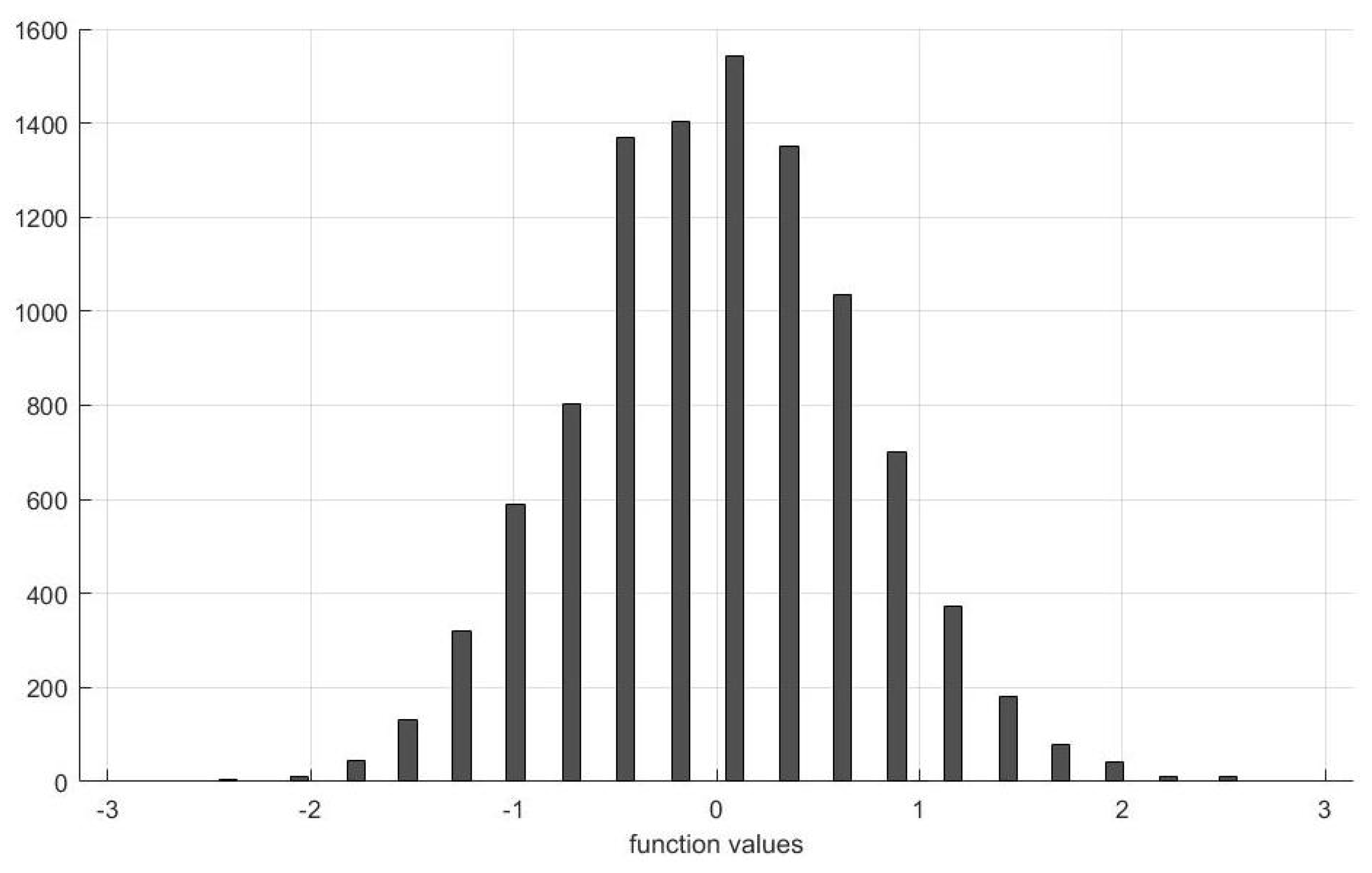
Because of the reason mentioned above, we have not been able to show the central limit theorem for the random variables or , the base of our series . Nevertheless, numerical computations strongly suggest that the central limit theorem holds; see Figure 9: we took uniformly-distributed points x of the interval and computed the sample average for 78,498, that is, the number of primes . We computed the histogram for the values of the sample average, which experimentally tends to a normal distribution as the size of the sample tends to infinity. To confirm this observation, we did the same computation for , see Figure 10.
4. Concluding Remarks
The properties of the series that we have discussed in this article are intimately related to the distribution of prime numbers, and this was mostly due to the unanswered questions on prime numbers for which the analytical access to our series is limited. Therefore, knowledge about the distribution and bounds for the gaps of prime numbers would imply more or less directly the properties where we were restricted to a numerical approach.
Although the series might be reminiscent of the Riemann zeta function or other number-theoretical functions, we did not construct in this way and do not see a possibility to deduce it from any of them, besides from the trivial fact, that is equal to the prime zeta function . Furthermore, recall that we only consider , usually , so that no zeros of the Riemann zeta function come into the play for the scope of this article.
Acknowledgments
We would like to thank Juri Merger and Florian Pausinger for his helpful hints and questions.
Author Contributions
D.V. conceived of and designed the experiments. D.V. and D.B. performed the experiments. D.V. and D.B. analyzed the data. D.B. wrote the paper.
Conflicts of Interest
The authors declare no conflict of interest.
References
- Cramér, H. On the order of magnitude of the difference between consecutive prime numbers. Acta Arith. 1936, 2, 23–46. [Google Scholar] [CrossRef]
- Vartziotis, D.; Wipper, J. The fractal nature of an approximate prime counting function. Fractal Fract. 2017, 1, 10. [Google Scholar] [CrossRef]
- Raseta, M. On the strong approximations of partial sums of f(nkx). arXiv, 2015; arXiv:1509.08138. [Google Scholar]
- Philipp, W.; Stout, W.F. Almost Sure Invariance Principles for Partial Sums of Weakly Dependent Random Variables; American Mathematical Society: Providence, RI, USA, 1975. [Google Scholar]
- Hardy, G.H. Weierstrass’s Non-Differentiable Function. Trans. Am. Math. Soc. 1916, 17, 301–325. [Google Scholar]
- Jaffard, S. Pointwise and directional regularity of nonharmonic Fourier series. Appl. Comput. Harmon. Anal. 2010, 22, 251–266. [Google Scholar] [CrossRef]
- Hardy, G.H.; Littlewood, J.E. Contributions to the arithmetic theory of series. Proc. Lond. Math. Soc. 1913, 2, 411–478. [Google Scholar] [CrossRef]
- Gerver, J. The differentiability of the Riemann function at certain rational multiples of π. Am. J. Math. 1970, 92, 33–55. [Google Scholar] [CrossRef]
- Gerver, J. More on the differentiability of the Riemann function. Am. J. Math. 1970, 93, 33–41. [Google Scholar] [CrossRef]
- Chamizo, F.; Córdoba, A. Differentiability and dimension of some fractal Fourier series. Adv. Math. 1996, 142, 335–354. [Google Scholar] [CrossRef]
- Landau, E.; Walfisz, A. Über die nichfortsetzbarkeit einiger durch dirichletsche reihen definierter funktionen. Rendiconti del Circolo Matematico di Palermo 1920, 44, 82–86. (In German) [Google Scholar] [CrossRef]
- Fröberg, C.E. On the prime zeta function. BIT 1968, 8, 187–202. [Google Scholar] [CrossRef]
- Rosser, J.; Schoenfeld, L. Approximate formulas for some functions of prime numbers. Ill. J. Math. 1962, 6, 64–94. [Google Scholar]
- Cohen, H. High Precision Computation of Hardy-Littlewood Constants. 2000. Available online: https://www.math.u-bordeaux.fr/~hecohen/ (accessed on 1 January 2018).
- Cattani, C. Fractal patterns in prime numbers distribution. In Lecture Notes in Computer Science, Proceedings of the International Conference on Computational Science and Its Applications (ICCSA 2010), Fukuoka, Japan, 23–26 March 2010; Taniar, D., Gervasi, O., Murgante, B., Pardede, E., Apduhan, B.O., Eds.; Springer: Berlin/Heidelberg, Germany, 2010; Part II, pp. 164–176. [Google Scholar]
- Cattani, C.; Ciancio, A. On the fractal distribution of primes and prime-indexed primes by the binary image analysis. Phys. A Stat. Mech. Its Appl. 2016, 460, 222–229. [Google Scholar] [CrossRef]
- Kahane, J.P. A century of interplay between taylor series, Fourier series and brownian motion. Bull. Lond. Math. Soc. 1997, 29, 257–279. [Google Scholar] [CrossRef]
- Salem, R.; Zygmund, A. On lacunary trigonometric series. Proc. Natl. Acad. Sci. USA 1947, 33, 333–338. [Google Scholar] [CrossRef] [PubMed]
- Salem, R.; Zygmund, A. On lacunary trigonometric series, II. Proc. Natl. Acad. Sci. USA 1948, 34, 54–62. [Google Scholar] [CrossRef] [PubMed]
- Erdös, P.; Gál, I. On the law of iterated logarithm I + II. Indag. Math. (Proceedings) 1955, 58, 65–84. [Google Scholar] [CrossRef]
- Weiss, M. The law of the iterated logarithm for lacunary trigonometric series. Trans. Am. Math. Soc. 1959, 91, 444–469. [Google Scholar]
- Erdös, P. On trigonometric sums with gaps. Magyar Tud. Akad. Mat. Kutató Int. Közl 1962, 7, 37–42. [Google Scholar]
- Gaposhkin, V.F. Lacunary series and independent functions. Uspekhi Matematicheskikh Nauk 1966, 21, 3–82. [Google Scholar] [CrossRef]
- Berkes, I.; Philipp, W.; Tichy, R. Metric discrepancy results for sequences {nkx} and diophantine equations. In Diophantine Approximation: Festschrift for Wolfgang Schmidt; Springer: Vienna, Austria, 2008; pp. 95–105. [Google Scholar]
- Goldston, D.A.; Pintz, J.; Yildirim, C.Y. Primes in tuples I. Ann. Math. 2009, 170, 819–862. [Google Scholar] [CrossRef]
- Schatte, P. On a law of iterated logarithm for sums mod 1 with applications to Benford’s law. Probab. Theory Relat. Fields 1988, 77, 167–178. [Google Scholar] [CrossRef]
Figure 1.
Graph of (a): with and and (b): with and (displayed for at points).

Figure 2.
Graph of (a):; (b): ; (c): (displayed for at points).

Figure 3.
Graph of at discrete points in each direction (interpolated).
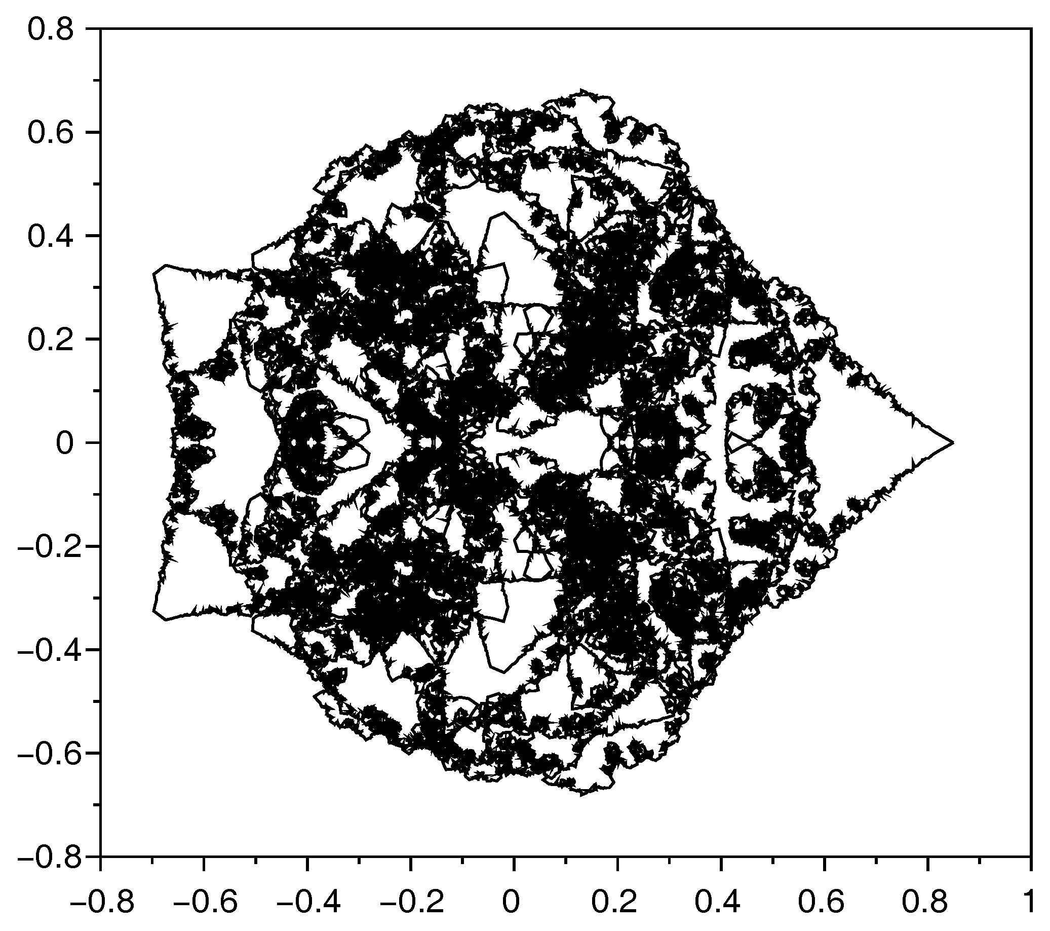
Figure 4.
Graph of at discrete points in each direction (interpolated).
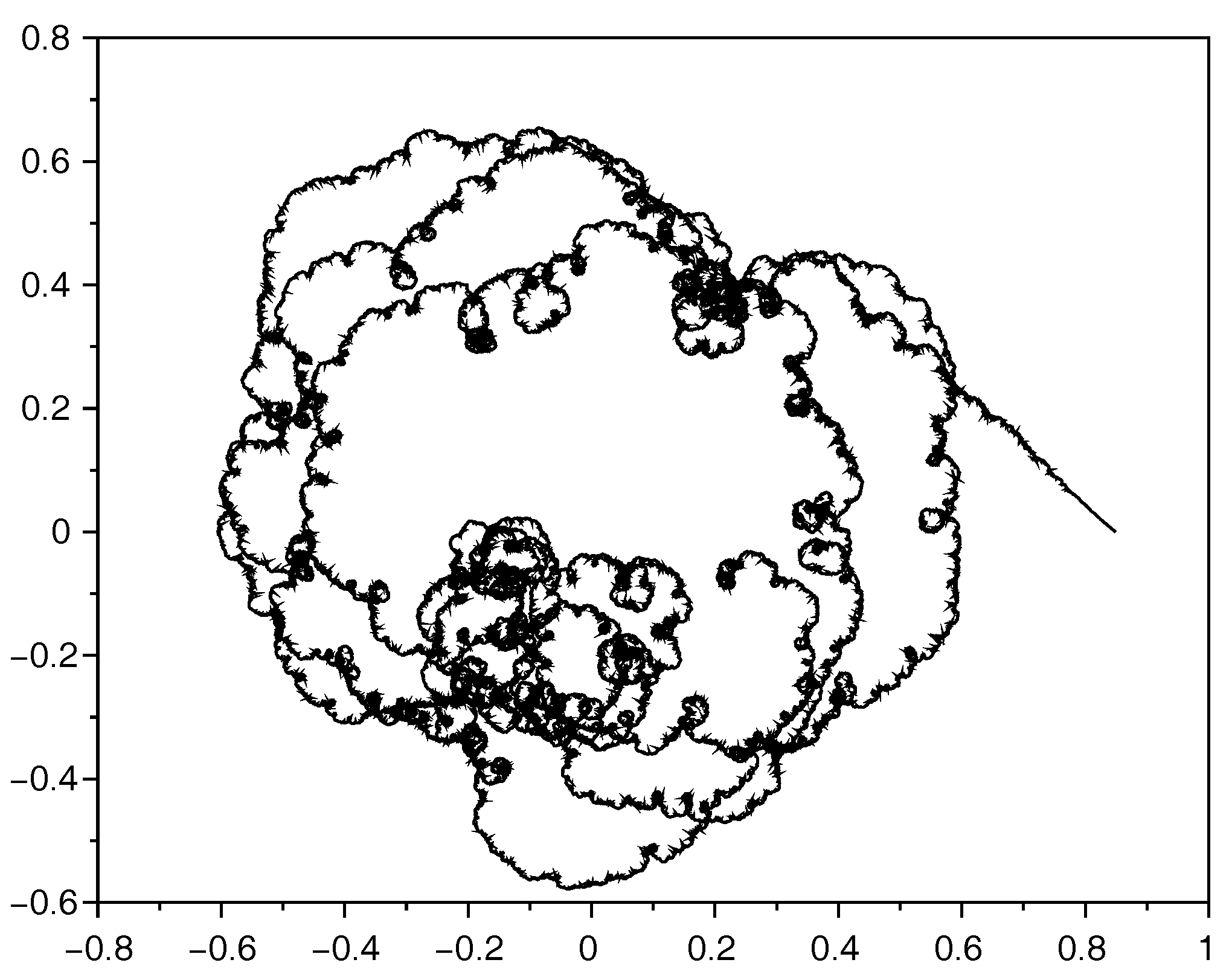
Figure 5.
Graph of at discrete points in each direction (interpolated).

Figure 6.
Graph of at discrete points.

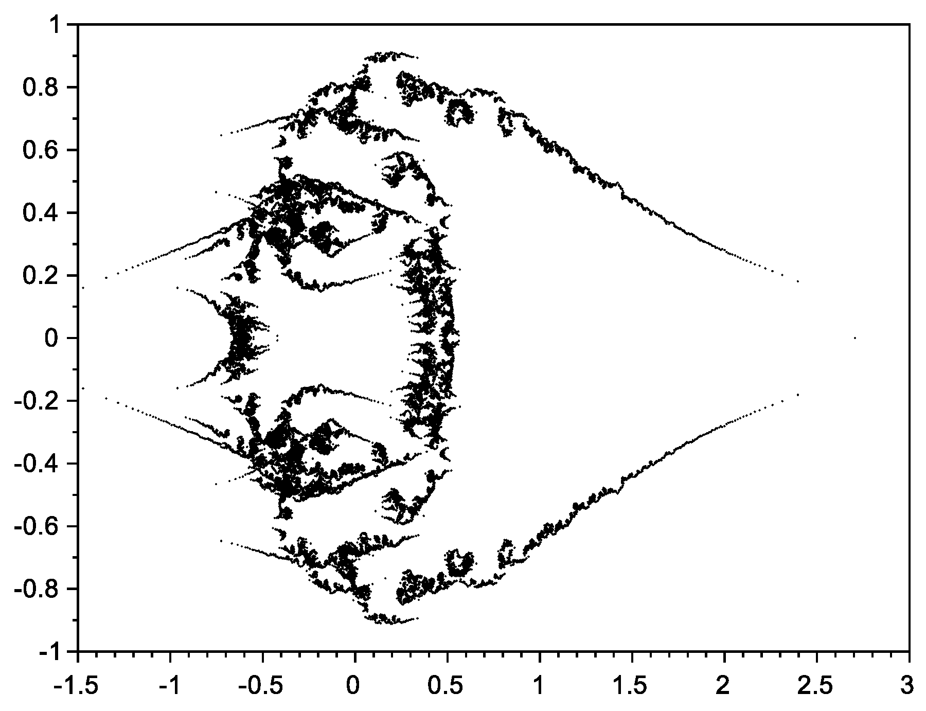
Figure 7.
The graph of the real part of (in black) and (in green).

Figure 8.
(a): Box dimension for the graph of (computed at points) in dependence of the fraction of the powers with and . Remark that is not convergent for . (b): example for to show how the box dimension was numerically approximated.
Figure 8.
(a): Box dimension for the graph of (computed at points) in dependence of the fraction of the powers with and . Remark that is not convergent for . (b): example for to show how the box dimension was numerically approximated.

Figure 9.
Normal distribution of for x uniformly distributed in .
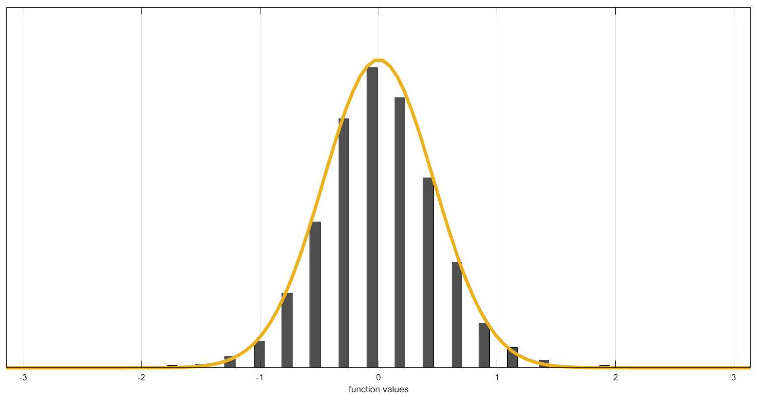
Figure 10.
Normal distribution of for x uniformly distributed in .
© 2018 by the authors. Licensee MDPI, Basel, Switzerland. This article is an open access article distributed under the terms and conditions of the Creative Commons Attribution (CC BY) license (http://creativecommons.org/licenses/by/4.0/).
Share and Cite
MDPI and ACS Style
Vartziotis, D.; Bohnet, D. Fractal Curves from Prime Trigonometric Series. Fractal Fract. 2018, 2, 2. https://doi.org/10.3390/fractalfract2010002
AMA Style
Vartziotis D, Bohnet D. Fractal Curves from Prime Trigonometric Series. Fractal and Fractional. 2018; 2(1):2. https://doi.org/10.3390/fractalfract2010002
Chicago/Turabian StyleVartziotis, Dimitris, and Doris Bohnet. 2018. "Fractal Curves from Prime Trigonometric Series" Fractal and Fractional 2, no. 1: 2. https://doi.org/10.3390/fractalfract2010002