Monitoring Liquid-Liquid Mixtures Using Fractional Calculus and Image Analysis


1
Departamento de Física, Universidade Estadual de Ponta Grossa, Av. Carlos Cavalcanti, 4748, Ponta Grossa 84030-900, Paraná, Brazil
2
Departamento de Transportes, Universidade Federal do Paraná, Rua Coronel Francisco H. dos Santos, 100, Curitiba 81531-980, Parana, Brazil
3
Departamento de Engenharia Química, Universidade Federal do Paraná, Rua Coronel Francisco H. dos Santos, 100, Curitiba 81531-980, Parana, Brazil
*
Author to whom correspondence should be addressed.
Fractal Fract. 2018, 2(1), 11; https://doi.org/10.3390/fractalfract2010011
Submission received: 28 December 2017
/
Revised: 6 February 2018
/
Accepted: 8 February 2018
/
Published: 11 February 2018
(This article belongs to the Special Issue The Craft of Fractional Modelling in Science and Engineering)
Abstract
:A fractional-calculus-based model is used to analyze the data obtained from the image analysis of mixtures of olive and soybean oil, which were quantified with the RGB color system. The model consists in a linear fractional differential equation, containing one fractional derivative of order α and an additional term multiplied by a parameter k. Using a hybrid parameter estimation scheme (genetic algorithm and a simplex-based algorithm), the model parameters were estimated as k = 3.42 ± 0.12 and α = 1.196 ± 0.027, while a correlation coefficient value of 0.997 was obtained. For the sake of comparison, parameter α was set equal to 1 and an integer order model was also studied, resulting in a one-parameter model with k = 3.11 ± 0.28. Joint confidence regions are calculated for the fractional order model, showing that the derivative order is statistically different from 1. Finally, an independent validation sample of color component B equal to 96 obtained from a sample with olive oil mass fraction equal to 0.25 is used for prediction purposes. The fractional model predicted the color B value equal to 93.1 ± 6.6.
1. Introduction
Process monitoring represents an important and fundamental tool aimed at process safety and economics while meeting environmental regulations. However, for suitable process monitoring, the analytical instrumentation remains a challenge due to higher costs, equipment sensitivity, and level of detection, among others [1]. In order to overcome some of these difficulties, image analysis represents an important field of process monitoring [2]. The main advantages and features are the low cost, non-invasive characteristics, and high precision/accuracy [3]. The literature reports a broad range of image analysis applications to food science [4], medical science [5], road-traffic monitoring [6], road pavement monitoring [7], flare combustion [8], and composition monitoring [9]. Additionally, applications in the quantification of edible oils mixtures, which have applications in many processes, such as biodiesel synthesis [10], pavement rejuvenating agents [11,12], and polyurethane synthesis [13], has also been reported. In this sense, Fernandes et al. [14] analyzed olive and soybean oil mixtures using image analysis (RGB color system) with linear models for a range of olive oil mass fraction of 0–0.7. When coupling the image analysis to Ultraviolet–visible spectroscopy (UV–VIS) spectra, successful predictions in the range of olive oil mass fraction of 0–1 could be obtained. Therefore, the use of nonlinear models would avoid the use of the UV–VIS spectra in order to accurately predict the mixture content, as the values of one of the color components behaved as an exponential decay with an increase in the olive oil content. This would be an important feature as experimental steps would vanish, therefore, leading to faster and cheaper results.
Towards this, a mathematical model that consists of a linear fractional differential equation is proposed. It contains one fractional derivative of order α and one other linear term multiplied by a parameter k. It was used to analyze the Fernandes et al. [14] experimental data. It is worth mentioning that fractional calculus deals with differential operators of arbitrary order, being an important tool to describe memory and hereditary effects of properties of many materials and processes [15]. Fractional calculus also presents a broad range of applications in process systems engineering, rheology, viscoelasticity, acoustics, optics, chemical physics, robotics, electrical engineering, bioengineering, anomalous diffusion [16,17,18,19,20,21]. The solution of the model here proposed is a nonlinear algebraic equation based on the Mittag-Leffer function, which according to the value of parameter α can turn into, for example, an exponential function. We also performed a comparison with an integer order model in order to show that the fractional derivative order is more suitable to describe the experimental data behavior.
2. Materials and Methods
The experimental data previously reported by Fernandes et al. in [14] concerning the off-line monitoring of mixtures of olive and soybean oil was used in this manuscript. To summarize, Fernandes et al. [14] used the RGB color system for off-line image analysis, where a given number of samples was used for parameter estimation of linear models aimed at concentration prediction and an independent sample was used for validation purposes, further details can be found in reference [14]. Below, the Table 1 presents the experimental data used in this work.
The main idea of the model is to consider the color component B as a function of the mass fraction (mf) of the olive oil in the mixture, as if it would be “disappearing” with an increase of the olive oil content. Secondly, it is assumed that the color component behavior follows the fractional differential equation of order α, subjected to the initial conditions given by B(mf = 0) = B0 and :
where the fractional derivative operator considered here is the Caputo [22] sense, defined as , with and (n − 1) < α < n, where n is an arbitrary integer number, and α is a real number.
The solution of Equation (1) can be obtained by using the Laplace Transform Method and it can be expressed in terms of the Mittag-Leffer function [23] as follows:
where Γ is the Gamma function (see Equation (17)). It is important to observe that for α = 1, Equation (2) turns into an integer order model (for B(mf = 0) = B0), which basically concerns an exponential variation of the color component, i.e.:
The parameter estimation procedure considers a hybrid task aimed at minimizing the least square function, given by:
where NE is the number of experimental data, EXP refers to experimental data and MOD refers to model predictions and delta is the difference between experimental data and model predictions.
A genetic algorithm, based on Isfer et al. [24], was firstly used and the results of this initial estimation step were used as the initial guess of a simplex-based method [25], in order to refine the solution. The main role of the genetic algorithm is to avoid a local minimum of the objective function. Regarding the integer order model, the parameter estimation task used the following expression as an objective function:
The statistical analysis of the estimated parameters and the mathematical model itself followed previously-reported procedures [26,27,28]. The parametric variance matrix, , is defined as for the fractional order model, where parameters α and k need to be estimated. From this matrix one can obtain the standard deviation of the model parameters:
Regarding the integer order model, the parameter variance is given by:
where only the parameter k needs to be estimated.
From the parametric variance matrix, one can obtain the parametric correlation matrix, given by:
for the fractional order matrix, while for the integer order matrix, this matrix does not exist as the model has only one parameter. It is important to emphasize that the experimental errors (variance) are considered constant and equal for all experimental data and its value is adequately predicted by:
where NE is the number of experiments and NP is the number of parameter to be estimated (“k” and “α” (alpha) in the case of the fractional model and “k” in the case of the integer order model). Note that a better value of the experimental error can be obtained by experimental runs carried out in triplicate or quadruplicate.
Therefore, an experimental variance matrix, , can be obtained, given by Equation (10), where is a square identity matrix of dimension NE × NE:
According to the literature [24,25,26,27,28], the elements of the matrix given by Equations (6) and (7) are given by Equation (11):
where is the Hessian matrix of the objective function (Equation (4) or Equation (5)) where the derivatives were obtained with respect to the parameters and is the Hessian matrix of the model (Equation (2) or Equation (3)) where the derivatives were also obtained with respect to the parameters. As the model predictions are usually close to the experimental values, deltai(mf) is close to zero, the parametric variance matrix is commonly simplified [28] to the following equation:
The sensitivity matrix G, present in Equation (12), regarding the fractional order model can be written as:
Concerning the integer order model, it is given by:
Considering the fractional case, the model derivatives c with respect to the parameters are given by the expressions:
where the relations defined below are valid [29], where x and t are dummy variables:
On the other hand, considering the integer order model, the model derivative with respect to the parameter is given by Equation (18):
The parameters confidence intervals are calculated by:
for the fractional order model and by:
for the integer order model. The parameter standard deviation is obtained from the square root of the elements of the diagonal of the matrix given by Equation (12). Additionally, for a given confidence level (usually 95%, therefore, β equals 0.05) and the degree of freedom (NE–NP), the Student’s t distribution value is used to obtain the formal confidence interval.
The parameter joint confidence region of the fractional order model is given by:
where the value of the Fisher distribution value, F, is obtained for a given confidence level (usually 95%, therefore β equals 0.05) and the degrees of freedom NP and (NE−NP). In the previous equation, the approximation given by Equation (12) is considered, consequently, Equation (22), is used in this work for the fractional order model:
It is important to emphasize that the region calculated by the equation
usually has an ellipsoidal shape due to the presence of parameter correlation and corresponds to a linearization of the objective function [24,25,26,27,28].
A more realistic parametric joint confidence region can be obtained by Equation (24), where the nonlinear feature of the objective function is taken into account. It is important to stress that the region calculated by Equation (24) is larger than the region obtained by Equation (23) and it does not necessarily has an ellipsoidal shape [30]:
where FOBJ(kestimated, αestimated) is the final value of the objective function.
The correlation coefficient between model predictions and experimental data, r, is:
Finally, regarding the fractional order model, the variance of model predictions of the experimental data used in the parameter estimation task, named in this work as model confidence region, is given by Equations (26) and (27). If the confidence interval of future experimental data prediction is necessary, Equations (28) and (29) should be used instead as, in this case, both the experimental error and the model error prediction should be considered. The following equations were also used for the integer order model analysis:
3. Results
For the genetic algorithm, the number of individuals (each individual consist on a pair of k, α for the fractional order model, or a single value of k for the integer order model) was set equal to 200 and the number of generations was set equal to 100. The probabilities of crossover and mutation were set as 80% assuring a good macroscopic search and of 10% assuring a good microscopic (refinement), respectively. In order to obtain each individual of a given generation, two individuals (“genitors”) of the previous generation were randomly selected. After that, a random number in the interval (0–1) was generated, and if its value was in the interval of (0–0.8), the crossover, which consisted in an arithmetic mean of the values of the parameters of the genitors, occurred, leading to a new individual. If a number between (0.8–1) was generated, the genitor with the lowest objective function was selected as the new individual of the current generation. Afterwards, another random number in the interval (0–1) was generated. If its value was in the interval of (0–0.15), mutation occurred. The mutation consisted in increasing the parameter value resulting from the crossover step by 10% of its value. If a number between (0.15–1) was generated, no mutation occurred. For another individual, two new different genitors were randomly selected. Finally, it is important to mention that 10 independent runs were carried out using the genetic algorithm. The simplex-based model used 10−5 as the convergence criteria for all parameters. Table 2 presents the parameter estimation results.
From the results reported in Table 2, one can verify that the fractional order model can successfully describe the experimental dataset and it also shows to be a better model than the integer order model. This can be observed by the lower values of the objective function, the parametric variance, the narrower confidence interval and the closer to one value of the correlation coefficient presented by the fractional order model. One can conclude that this better fit occurred because the integer order model has a one parameter, while the fractional order model has two parameters. However, the value of is a more neutral comparison value, as it takes into account the number of parameters of the model, this value was also smaller for the fractional order model. Finally, it is important to stress that parameter α is not a simple fitting parameter. It also shapes the mathematical function during the estimation task, according to the value of α the Mittag-Leffler function assumes a different mathematical form. As mentioned, if α = 1, an exponential function shows up, while if α ≠ 1, another function is represented by the Mittag-Leffler expression. It is important to observe from Table 2 that the parametric correlation between k and α is approximately 0.3, which is an important result as the final value of parameter k has little influence on the final value of parameter α. According to Himmelblau [27], when the parametric correlation is close to 1 or −1, a wrong set of parameters can be estimated as a wrong value of one parameter could be compensated by a wrong value of another parameter resulting in an overall good fit. Consequently, the lower the parametric correlation, the closer to the true value the parameters tend to be. Finally, it is important to mention that the confidence interval of the fractional differential equation order, parameter α, [1.14; 1.26] does not include the value 1, therefore, it is very important to stress that the fractional derivative is statistically different from an integer order derivative.
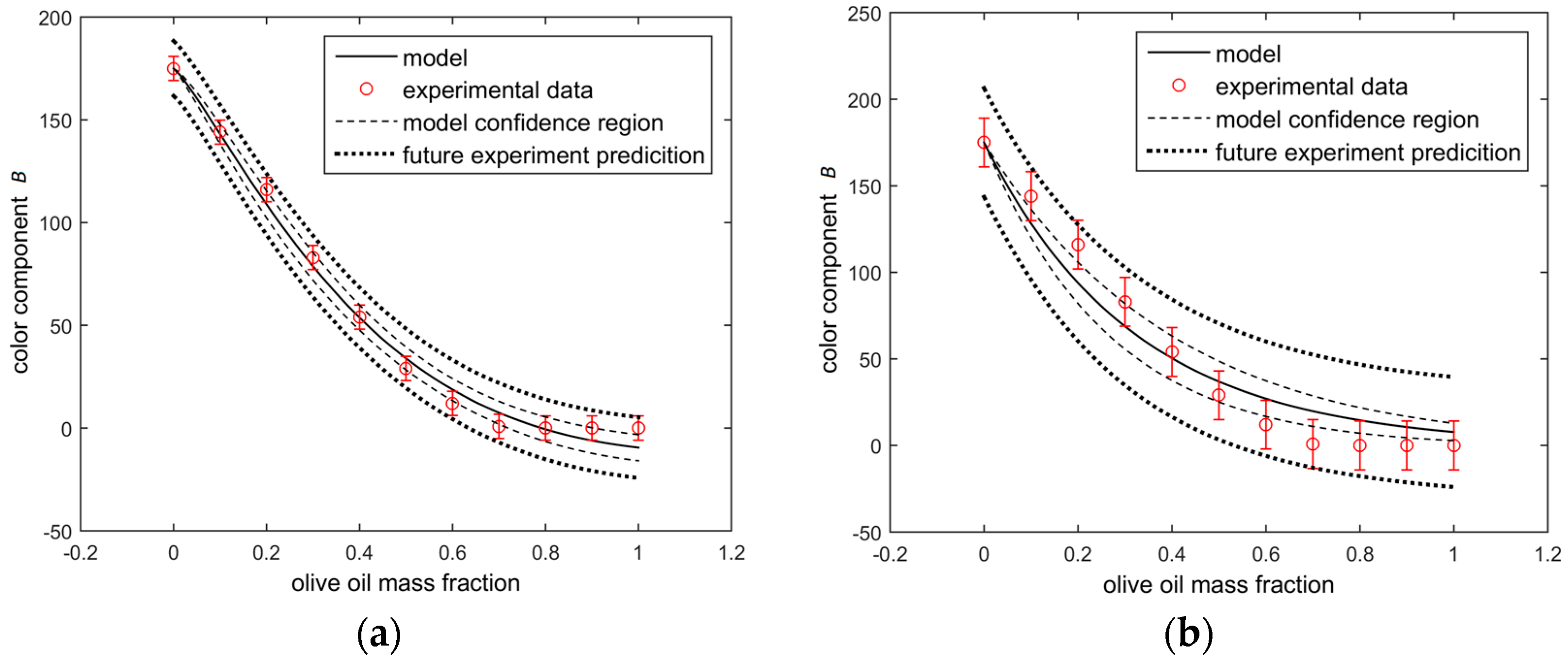
Figure 1 compares the model behavior of both modeling approaches. The better fit provided by the fractional order model (Figure 1a) can be seen, as the model is closer to the experimental data when compared to the integer order model (Figure 1b). This happened as a result of the parameter estimation results listed in Table 2. Additionally, one can observe that the model confidence regions and model prediction regions are narrower in the fractional order model. As this model provided a better fit, the confidence in the model predictions tend to be closer to the true value. Finally, it is important to observe that the integer order model is an exponential function, while the fractional order model is a different function, as the value of α is different from 1. In the figures, the vertical bar errors were calculated by Equation (9) for each model, and as the value of the objective function is smaller for the fractional order model, the experimental error prediction is also smaller. The model confidence region was obtained by Equation (26) and the region of future experiment prediction was calculated by Equation (28). This last region is expected to be broader as it includes not only the model variance, but also the experimental variance.
Figure 2 compares the model predictions and the experimental data of the fractional order model (Figure 2a) and the integer order model (Figure 2b). The vertical bar errors were calculated by Equation (9) and the horizontal bar errors were obtained by Equation (30). It can be seen that the model predictions of the fractional order model are closer to the experimental values:
Figure 3 presents the histogram of residuals (difference between experimental data and model prediction) for the fractional order model (Figure 3a) and the integer order model (Figure 3b). It can be observed that, due to the better fit of the fractional order model, its residual histogram presents a narrower distribution and according to the mean and standard deviation, and one can conclude that the average residual is equal to zero (the standard deviation is much higher than the mean). This is an important feature, because an eventual difference may occur due to experimental error and not due to a biased model.
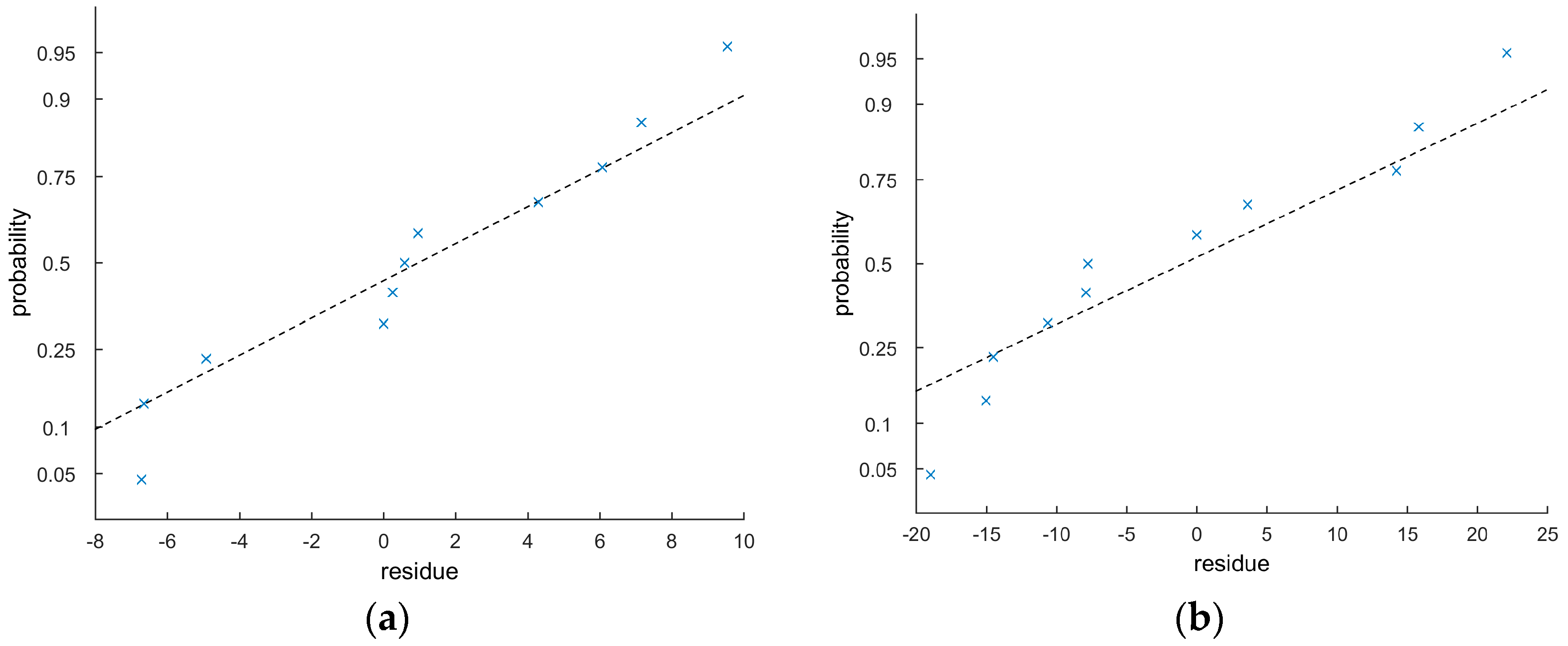
Figure 4 presents the normal probability plot of the residuals for the fractional order model (Figure 4a) and the integer order model (Figure 4b). One can observe that the residuals, besides having a mean value statistically equal to zero, can also be regarded as following a normal distribution, evidencing that the model predictions are not biased, i.e., the model does not need another term or parameter in its structure.
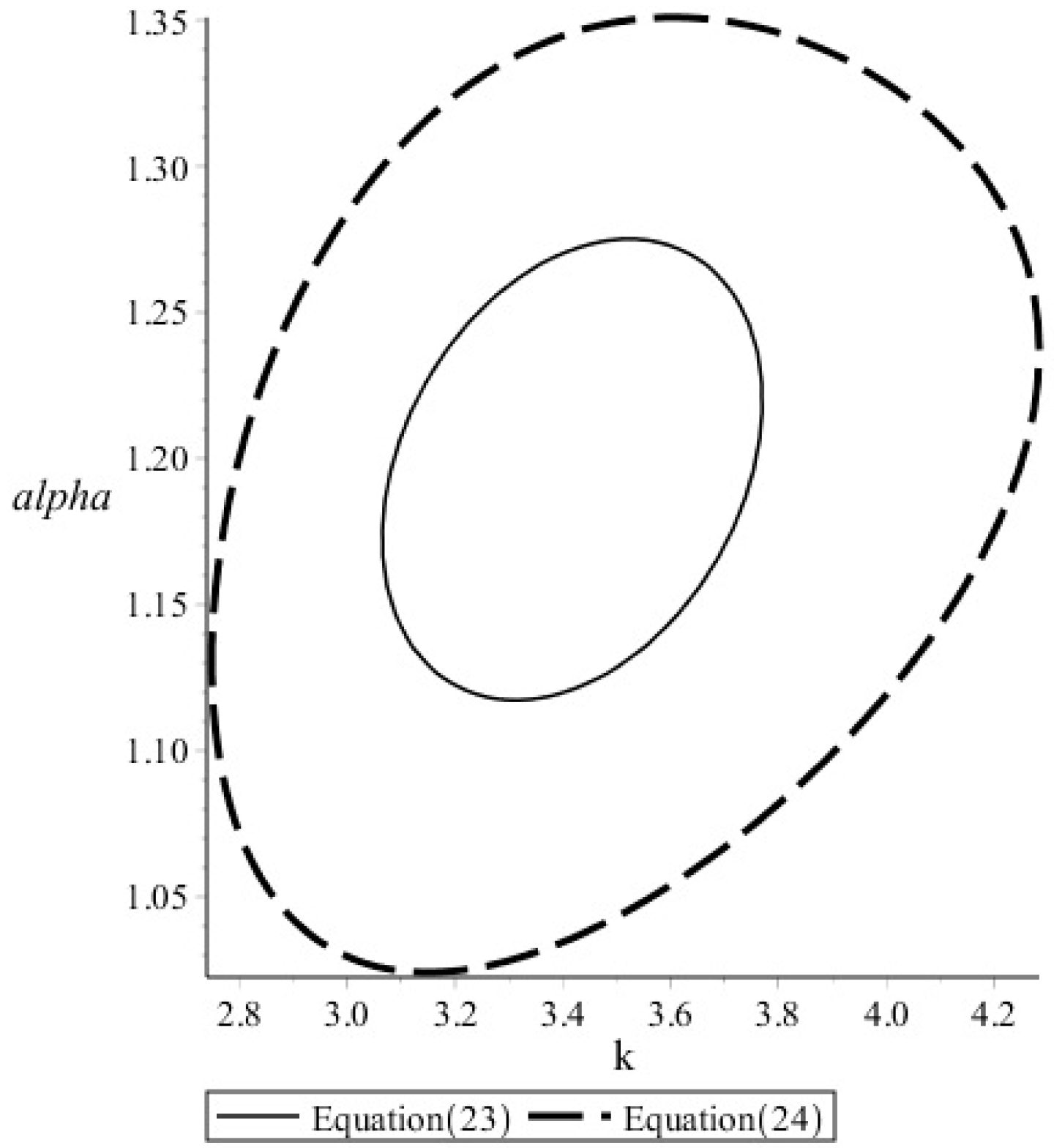
Figure 5 presents the joint confidence region calculated using the linear (Equation (23)) and nonlinear (Equation (24)) features of the objective function. The meaning of this region is that any set of parameters inside the region provides a statistically equal value of the objective function that another set of parameters would provide. Therefore, as mentioned before, it is important to stress that the values of parameter α (alpha) do not include the value 1, consequently, the value of the derivative is statistically different from an integer value. As expected, the region obtained by Equation (23) has an ellipsoidal shape and it is smaller than the region obtained by Equation (24), which considers the nonlinearities of the objective function.
Finally, Table 3 presents the model validation results. The model prediction for an olive oil mass fraction of 0.25 has a Color Component B of 93.1, which is close to the experimental value of 96. However, when considering the uncertainty of the model prediction, calculated using Equation (29), it can be regarded as statistically equal to the experimental value. The integer order model prediction is considerably different form the experimental value and the uncertainty of this prediction is even worse, which is one more indication that the fractional order model provides a better description of the experimental data and can be used for composition monitoring.
4. Conclusions
Two different models were used to quantify different olive and soybean oil mixtures characterized by image analysis with the aid of the RGB color system. The model based on the fractional calculus-based approach could better describe the experimental dataset, presenting better results of parameter estimation quantities, such as objective function values and parameter variance. This model could successfully describe an independent validation sample, while the integer order model failed to predict the value of the validation sample. Consequently, the approach proposed here can be used as an alternative tool for possible on-line monitoring applications where a change color occurs, and it can be processed and quantified by image analysis techniques.
Acknowledgments
The authors thank the financial support and scholarships provided by CAPES and CNPQ (Brazilian Agencies).
Author Contributions
Both authors equally contributed to all aspects during the development of this work and agree with the obtained results.
Conflicts of Interest
The authors declare no conflict of interest.
References
- Trevisan, M.G.; Poppi, R.J. Process Analytical Chemistry. Quim. Nova 2006, 29, 1065–1071. [Google Scholar] [CrossRef]
- Russ, J.C. The Image Processing Handbook, 6th ed.; CRC Press: Boca Raton, FL, USA, 1972; ISBN 978-1439840450. [Google Scholar]
- Liu, J.; Yang, W.W.; Wang, Y.S.; Rababah, T.M.; Walker, L.T. Optimizing machine vision based applications in agricultural products by artificial neural network. Int. J. Food Eng. 2011, 7, 1–23. [Google Scholar] [CrossRef]
- Zheng, C.X.; Sun, D.W.; Zheng, L.Y. Recent applications of image texture for evaluation of food qualities—A review. Trends Food Sci. Technol. 2006, 17, 113–128. [Google Scholar] [CrossRef]
- Litjens, G.; Kooi, T.; Bejnordi, B.E.; Setio, A.A.A.; Ciompi, F.; Ghafoorian, M.; van der Laak, J.A.W.M.; van Ginneken, B.; Sánchez, C.I. A survey on deep learning in medical image analysis. Med. Image Anal. 2017, 42, 60–88. [Google Scholar] [CrossRef] [PubMed]
- Fernández-Caballeroa, A.; Gómeza, F.J.; López-Lópeza, J. Road-traffic monitoring by knowledge-driven static and dynamic image analysis. Expert Syst. Appl. 2008, 35, 701–719. [Google Scholar] [CrossRef]
- Resende, M.R.; Bernucci, L.L.B.; Quintanilha, J.A. Monitoring the condition of roads pavement surfaces: Proposal of methodology using hyperspectral images. J. Transp. Lit. 2014, 8, 201–220. [Google Scholar] [CrossRef]
- Castiñeira, D.; Rawlings, B.C.; Edgar, T.F. Multivariate Image Analysis (MIA) for Industrial Flare Combustion Control. Ind. Eng. Chem. Res. 2012, 51, 12642–12652. [Google Scholar] [CrossRef]
- Licodiedoff, S.; Ribani, R.H.; Camlofski, A.M.O.; Lenzi, M.K. Use of image analysis for monitoring the dilution of Physalis peruviana pulp. Braz. Arch. Biol. Technol. 2013, 56, 467–474. [Google Scholar] [CrossRef]
- Ma, F.; Hanna, M.A. Biodiesel production: A review. Bioresour. Technol. 1999, 70, 1–15. [Google Scholar] [CrossRef]
- Moghaddam, T.B.; Baaj, H. The use of rejuvenating agents in production of recycled hot mix asphalt: A systematic review. Constr. Build. Mater. 2016, 114, 805–816. [Google Scholar] [CrossRef]
- Labegalini, A.; Teixeira, M.L.; Ryba, A.; Villena, J. Rejuvenescimento do Ligante Asfáltico CAP 50/70 Envelhecido com Adição de Óleo de Girassol. In Proceedings of the Reunião de Pavimentação Urbana, Florianópolis, Brazil, 28–30 June 2017. (In Portuguese). [Google Scholar]
- Tan, S.; Abraham, T.; Ference, D.; Macosko, C.W. Rigid polyurethane foams from a soybean oil-based polyol. Polymer 2011, 52, 2840–2846. [Google Scholar] [CrossRef]
- Fernandes, J.K.; Umebara, T.; Lenzi, M.K.; Alves, E.T.S. Image analysis for composition monitoring. Commercial blends of olive and soybean oil. Acta Sci. Technol. 2013, 35, 317–324. [Google Scholar] [CrossRef]
- Giona, M.; Roman, H.E. A theory of transport phenomena in disordered systems. Chem. Eng. J. 1992, 49, 1–10. [Google Scholar] [CrossRef]
- Hristov, J. Multiple integral-balance method basic idea and an example with mullin’s model of thermal grooving. Therm. Sci. 2017, 21, 1555–1560. [Google Scholar] [CrossRef]
- Ionescu, C.; Lopes, A.; Copot, D.; Machado, J.A.T.; Bates, J.H.T. The role of fractional calculus in modeling biological phenomena: A review. Commun. Nonlinear Sci. 2017, 51, 141–159. [Google Scholar] [CrossRef]
- Caratelli, D.; Mescia, L.; Bia, P.; Stukach, O.V. Fractional–Calculus–Based FDTD Algorithm for Ultrawideband Electromagnetic Characterization of Arbitrary Dispersive Dielectric Materials. IEEE Trans. Antennas Propag. 2016, 64, 3533–3544. [Google Scholar] [CrossRef]
- Chen, W.; Sun, H.; Zhang, X.; Korošak, D. Anomalous diffusion modeling by fractal and fractional derivatives. Comput. Math. Appl. 2010, 59, 1754–1758. [Google Scholar] [CrossRef]
- Fu, Z.-J.; Chen, W.; Yang, H.-T. Boundary particle method for Laplace transformed time fractional diffusion equations. J. Comput. Phys. 2013, 235, 52–66. [Google Scholar] [CrossRef]
- Evangelista, L.R.; Lenzi, E.K. Fractional Diffusion Equations and Anomalous Diffusion, 1st ed.; Cambridge University Press: Cambrigde, UK, 2018. [Google Scholar]
- Caputo, M. Linear models of dissipation whose Q is almost frequency independent-2. Geophys. J. R. Astron. Soc. 1967, 13, 529–538. [Google Scholar] [CrossRef]
- Podlubny, I. Fractional-order systems and PIλDµ controllers. IEEE Trans. Autom. Control 1999, 44, 208–214. [Google Scholar] [CrossRef]
- Isfer, L.A.D.; Lenzi, E.K.; Lenzi, M.K. Identification of biochemical reactors using fractional differential equation. Lat. Am. App. Res. 2010, 40, 193–198. [Google Scholar]
- Lagarias, J.C.; Reeds, J.A.; Wright, M.H.; Wright, P.E. Convergence properties of the Nelder–Mead simplex method in low dimensions. SIAM J. Optim. 1998, 9, 112–147. [Google Scholar] [CrossRef]
- Gomes, E.M.; Silva, F.R.G.B.; Araújo, R.R.L.; Lenzi, E.K.; Lenzi, M.K. Parametric Analysis of a Heavy Metal Sorption Isotherm Based on Fractional Calculus. Math. Probl. Eng. 2013, 642101. [Google Scholar] [CrossRef]
- Himmelblau, D.M. Process Analysis by Statistical Methods, 1st ed.; John Wiley & Sons: New York, NY, USA, 1970; ISBN 978-0471399858. [Google Scholar]
- Bard, Y. Nonlinear Parameter Estimation, 1st ed.; Academic Press: New York, NY, USA, 1974; ISBN 978-0120782505. [Google Scholar]
- Lebedev, N.N. Special Functions & Their Applications, 1st ed.; Dover Publications: New York, NY, USA, 1972; ISBN 978-0486606248. [Google Scholar]
- Box, G.E.P.; Hunter, W.G. A useful method for model building. Technometrics 1962, 4, 301–318. [Google Scholar] [CrossRef]
Figure 1.
(a) Fractional order model behavior; and (b) integer order model behavior.

Figure 2.
(a) Fractional order model behavior; and (b) integer order model behavior.
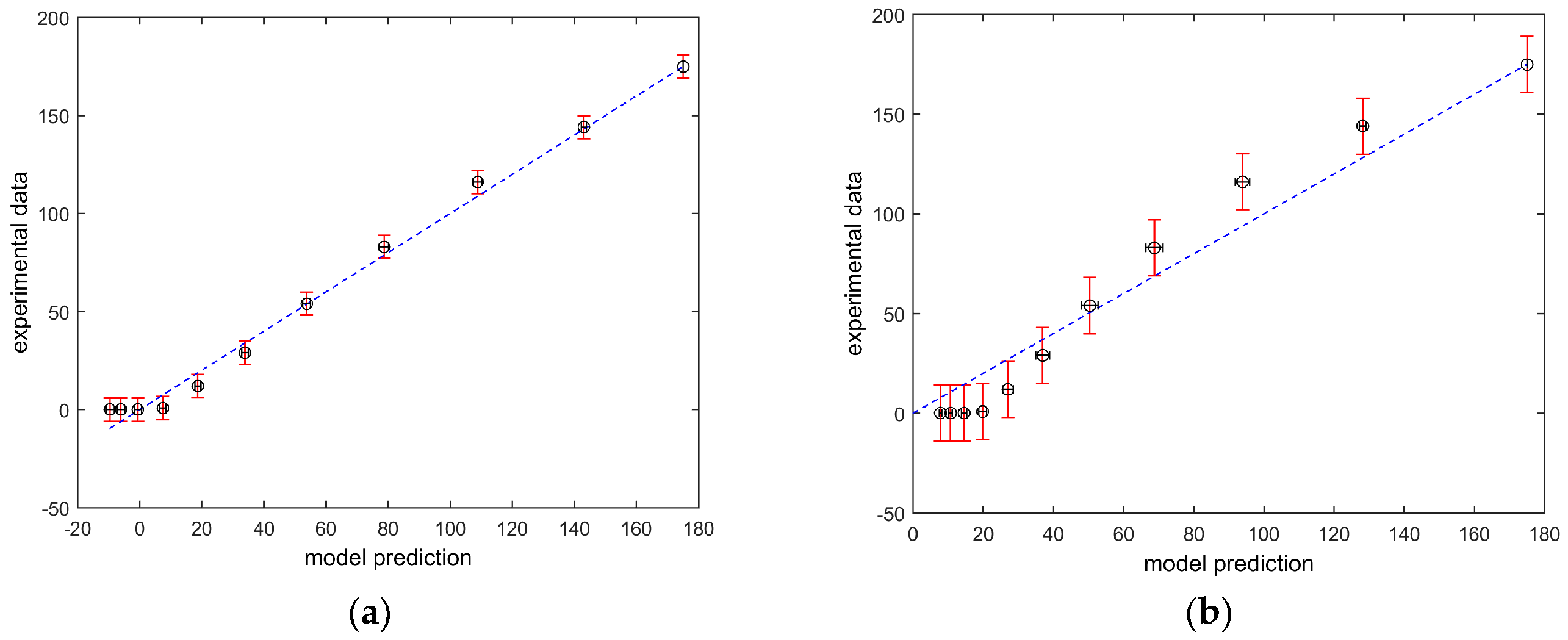
Figure 3.
(a) Fractional order model behavior; and (b) integer order model behavior.
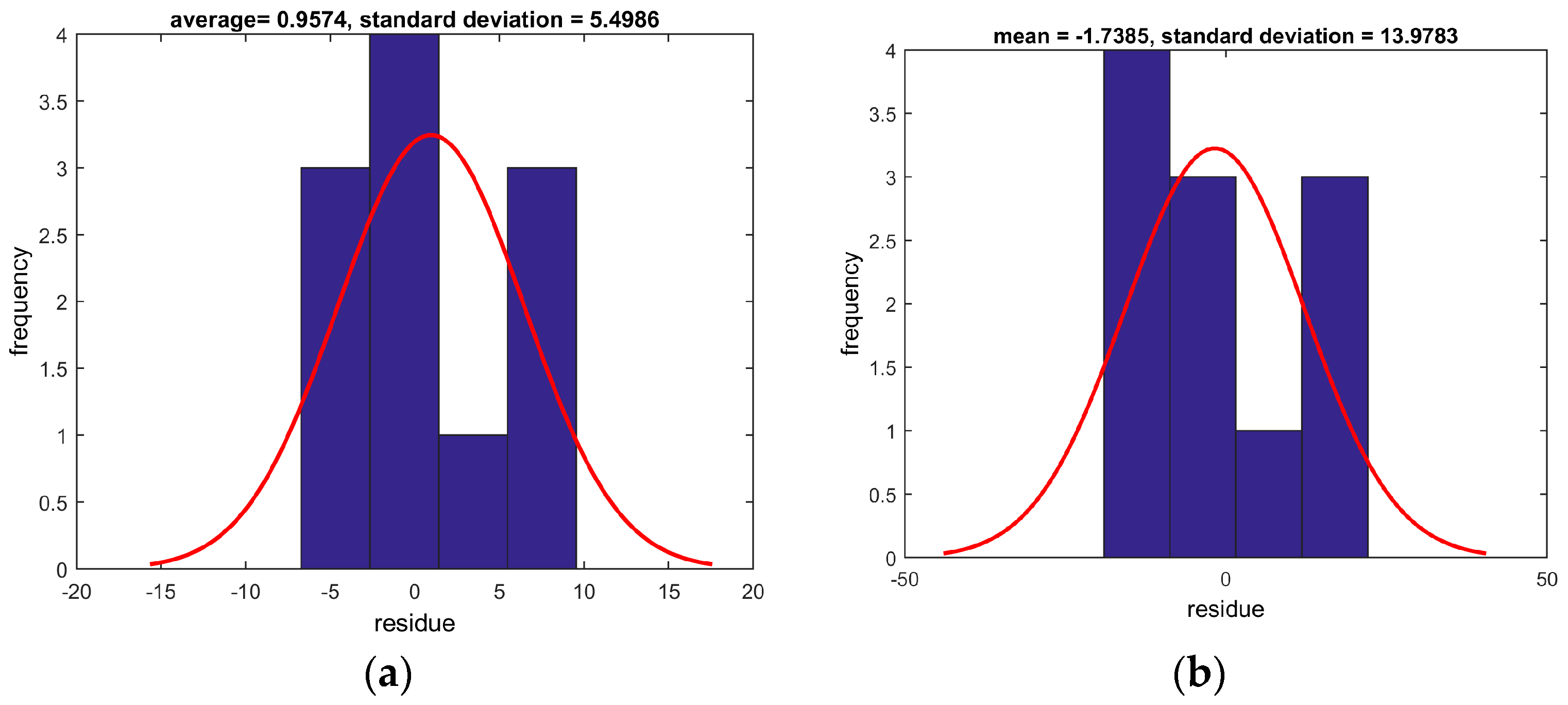
Figure 4.
(a) Fractional order model behavior; and (b) integer order model behavior.

Figure 5.
Joint confidence region.


Table 1.
Experimental data.
| Sample Purpose | Olive Oil Mass Fraction | Color Component B |
|---|---|---|
| Parameter Estimation | 0 | 175 |
| 0.1 | 144 | |
| 0.2 | 116 | |
| 0.3 | 83 | |
| 0.4 | 54 | |
| 0.5 | 29 | |
| 0.6 | 12 | |
| 0.7 | 0.8 | |
| 0.8 | 0 | |
| 0.9 | 0 | |
| 1 | 0 | |
| Model Validation | 0.25 | 96 |
Table 2.
Parameter estimation results.
| Result | Fractional Order Model | Equation | Integer Order Model | Equation |
|---|---|---|---|---|
| NE (Number of Experiments) | 11 | - | 11 | - |
| NP (Number of Parameters) | 2 (k, α) | - | 1 (k) | - |
| FOBJ | 312.4 | (4) | 1987.2 | (5) |
| 5.89 | (9) | 14.09 | (9) | |
| k | 3.42 | - | 3.11 | |
| k (standard deviation) | 0.12 | (6) | 0.28 | (7) |
| k (confidence interval) | [3.14; 3.69] | (19) | [2.48; 3.75] | (20) |
| α | 1.196 | - | - | - |
| α (standard deviation) | 0.027 | (6) | - | - |
| α (confidence interval) | [1.14; 1.26] | (19) | - | - |
| (parametric covariance matrix) | (6) | (7) | ||
| (parametric correlation matrix) | (8) | - | - | |
| r | 0.997 | (25) | 0.987 | (25) |
| r2 | 0.993 | - | 0.972 | - |
Table 3.
Model Validation.
| Experimental | Fractional Order Model Prediction | Integer Order Model Prediction | |
|---|---|---|---|
| Olive oil mass fraction | Color Component B | Color Component B | Color Component B |
| 0.25 | 96 | 93.1 ± 6.6 | 80.2 ± 15.2 |
© 2018 by the authors. Licensee MDPI, Basel, Switzerland. This article is an open access article distributed under the terms and conditions of the Creative Commons Attribution (CC BY) license (http://creativecommons.org/licenses/by/4.0/).
Share and Cite
MDPI and ACS Style
Lenzi, E.K.; Ryba, A.; Lenzi, M.K. Monitoring Liquid-Liquid Mixtures Using Fractional Calculus and Image Analysis. Fractal Fract. 2018, 2, 11. https://doi.org/10.3390/fractalfract2010011
AMA Style
Lenzi EK, Ryba A, Lenzi MK. Monitoring Liquid-Liquid Mixtures Using Fractional Calculus and Image Analysis. Fractal and Fractional. 2018; 2(1):11. https://doi.org/10.3390/fractalfract2010011
Chicago/Turabian StyleLenzi, Ervin K., Andrea Ryba, and Marcelo K. Lenzi. 2018. "Monitoring Liquid-Liquid Mixtures Using Fractional Calculus and Image Analysis" Fractal and Fractional 2, no. 1: 11. https://doi.org/10.3390/fractalfract2010011